A lake’s impact on suburban dwellings

(1)

Department of Economics

A lake’s impact on suburban dwellings

– a hedonic price study on housing in Täby

Johanna Berglund

Independent project • 15 credits

Economics and Management – Bachelor's Programme

Degree project/SLU, Department of Economics, 1223 • ISSN 1401-4084 Uppsala 2019

(2)

A lake´s impact on suburban dwellings

– a hedonic price study on housing in Täby

Johanna Berglund

Supervisor:

Examiner:

Vivian Wei Huang, Swedish University of Agricultural Sciences, Department of Economics

Jens Rommel, Swedish University of Agricultural Sciences, Department of Economics

Credits: 15 credits

Level: First cycle, G2E

Course title: Independent project in economics

Course code: EX0903

Programme/education: Economics and Management – Bachelor's Programme Course coordinating department:

Place of publication: Year of publication: Title of series: Part number: ISSN: Online publication: Keywords: Department of Economics Uppsala 2019 Degree thesis 1223 1401-4084 https://stud.epsilon.slu.se

Hedonic pricing, ecosystem services, nature, environmental attributes

Swedish University of Agricultural Sciences

Faculty of Natural Resources and Agricultural Sciences Department of Economics

(3)

iii

Acknowledgement

I would like to thank my supervisor Vivian Wei Huang for her support with all my questions throughout this study. I would also like to thank my parents for always believing in me and my friends for cheering on me on this journey.

(4)

iv

Abstract

Ecosystem services are of great interest for both cultural experiences, health benefits and keeping the earth living. With a growing population and increasing exploitation, it is crucial to recognize the value of natural sceneries to real estate in Sweden. This study aims to measure the willingness to pay for the distance from a house to the lake and that to the nearest forest area in the suburban municipality of Täby, Sweden. The Hedonic price method is used, which is a widely used model for valuation of non-market goods. The residential house sales prices for houses sold in 2014-2017, house characteristics, regional income, the distance to the lake Rönningesjön,the distance to the forest area - nature reserve Skavlöten, and other relevant information are obtained from website Booli, Hemnet, and Google maps. The results indicate that people would like to pay higher price for a closer distance to environmental attributes, in particular the distance to a lake. Robust estimation results show that the closer the distance between the house and the lake Rönningesjön the higher price of the house, and the cross-term for house type and lake distance also implies an additional price increase for detached houses. But the effect of the distance between the house and nature reserve Skavlöten is not robust. The results confirm that the residents value the local nature and would suggest further research on the valuation on cultural ecosystem services in urban environments.

(5)

v

1 Introduction

In this first part of the paper an introduction to the subject will be presented, followed by the research question and hypotheses and later a review of previous literature within the area of hedonic price models and environmental amenities.

1.1 Background

Ecosystem services are in all of its forms important for us humans. They provide us with fresh air, pollination and places for recreation just to name a few. Some of the services are taken for granted while others are more exploited. Numerous of these services are however non-market goods and are therefore difficult to put an exact monetary value on. Different models are used for estimating the economic value of environmental amenities. A widely used approach is to compare house prices with different levels of an amenity (Haab & McConnell 2002).

Forest and open areas are classed as cultural ecosystem services and provide recreational space for recovery and wellbeing for humans as well as decreasing the local temperature, stores water and provide shade on sunny days (Boverket 2019). Parks can indirectly promote health, by lowering particle levels in the air which is good for our bodies. Green areas create quiet spaces by absorbing sounds and are often used in urban areas to decrease noise pollutions which in turn reduce stress hormones and give us mental recovery (ibid). Easy access to recreational areas can increase the probability of physical activity, that will provide additional health benefits.

Sweden’s population is increasing and have increased from being just 9 million in mid 2004 to passing 10 million inhabitants in early 2017 (SCB 2019b). The country is becoming more urban, people move from rural areas or small towns to big cities where new areas need to be developed. When doing so, ecosystems and natural areas are put at risk of being ruined. Sweden has legislations regarding planning with requirements on municipalities and residents. The environmental laws sometimes require analyses on the impact an action could have on the environment within the area (see for instance Miljöbalk (1998:808) and Plan- och bygglag (2010:900)).

In the Stockholm suburb Täby new neighborhoods are built to supply the increasing population. The areas exploited are for instance former horse racing tracks and stables. When cities are

(8)

2

growing, and larger natural areas get harder to come by, it would be interesting to find out how cultural ecosystem services are valued today. Täby has two nature reserves, where Skavlöten is one. Nature reserves are formed to preserve important nature areas, landscapes and plant- and animal species for the future (Naturvårdsverket 2019)

This type of study, looking at environmental attributes and cultural ecosystem services in suburban areas in particular, have not been broadly done in Sweden. This study will therefore try to fill this gap.

1.2 Research question and hypothesis

The purpose of this paper is to investigate the valuation of different environmental attributes, in this case a lake and a forest area, by studying home sales prices in the municipality of Täby, Sweden. To display the willingness to pay for residence close to a natural scenery, the implicit prices will be estimated. This research will try to answer the following question;

- Which impact does closeness to recreational space, such as a lake or nature reserve, have on homes sales prices?

The hypothesis is that a decrease in distance to a natural scenery will positively affect home sales prices. Dwellings adjacent to the lake are expected to exhibit higher valuations than dwelling with further distances. Access to recreational areas and trails is more common than the more limited access to a lake or lake view and could therefore be valued less, however, it is still expected to have a positive relation to price.

1.3 Literature Review

In the following section previous literature, within the area of environmental attributes and Hedonic pricing, will be reviewed. Several studies have used the Hedonic price model as a way to measure the monetary value for non-market goods such as lake view and access to nature, by estimating the marginal value of a certain attribute.

Sander and Haight (2012) estimated the economic values of a number of cultural ecosystem services using the hedonic price model. The aim was to investigate how amenities such as scenic quality, open space and forest cover affected property prices in Dakota County, Minnesota. The

(9)

3 authors used ordinary least squares (OLS) to find the marginal implicit price change of a certain attribute. House and neighborhood characteristics, such as house age, lot size and school district, were used as independent variables as well. School district and the month in which the sale took place were used as dummy variables as a way to find differences between areas within the region. Single-family homes sales prices accounted as the dependent variable.

The model agreed with the expected signs of the variables and showed significant results regarding distance to a lake and open space. For one, increasing the distance to a park or a lake would have a negative effect on house price and increasing the open space view would have a positive effect on sales price. As the initial distance of 1km to an open space decreased with 100 meters, responded with the marginal implicit price increase of $13.16, or 0.040%, to the mean sales price. A 100m decrease to a lake increase mean sales price with $129, or 0.041%. The results also showed the impacts of open space view on home sales prices. An addition of 1ha (10 000m2_{) open space view to the mean view area, increased the price with $181, or}

0.057%. Both view over lawn and water also significantly affected sales prices positively, where a 1ha view increase responded with a $1742 (0.55%) and $81 (0.03%) respectively. Sander and Haight argue that cultural ecosystem services are important to local residents and that they are willing to pay for these amenities. However, since house related variables, such as number of rooms, were omitted the results could be bias.

In a similar article by Lutzenhiser and Netusil (2001), the aim was to find the relationship between different types of open space and home´s sales price. The authors compared sales prices of 16 636 houses sold in 1990-1992 within 1500 feet (457.2 meters) of open spaces in Portland. By using the hedonic price model, the price effect of a park or open space on house sales prices could be found. The 201 open spaces within the area were grouped into five categories and used as dummy variables in the later used model; urban parks, specialty park, natural area park, cemetery and golf course.

Two models were used, one to reflect each categories effect on sales prices, the second one measured different distances effect on price. It was found that natural park had the highest and urban parks the lowest significant impact on sales prices, $10 648 and $1214 respectively in 1990 dollars, with remaining variables held constant. Specialty parks and golf courses also showed significant effects, all four at the 1% level. The second model found that a natural area park within a 401-600 feet (122.2-182.8m) distance and a golf course within 200 feet had the

(10)

4

largest effect, $11 210 and $13 916 respectively. Overall, natural area parks indicated the strongest effect for all distance intervals while urban parks had smaller, but still positive, price effects, some of which were not significant. As Lutzenhiser and Netusil address, urban areas can be affected by other factors such as noise pollution. Traffic noise were included as a variable in the first model and indicated the marginal implicit price -$5242 for heavy traffic.

In a study by Hörnsten and Fredman (2000), the valuation for distance to a recreational forest was examined. The authors conducted a survey to find the present and the preferred distance to the closest forest; the willingness to pay (WTP) for not doubling the present distance; and the means of transportation. This survey was sent to two random selected sample groups of 500 people each in 1998 and they used the contingent valuation method for estimations. Hörnsten and Fredman found that 40.6% of all responders wished for a shorter distance, 48.8% did not wish for a change in distance at all and that 18.6% in the first sample would visit the forest more often if the distance was shorter. While some of the responders lived in areas with longer distances to forest areas, the majority of the responders lived in areas with higher tree cover and closer to recreational areas. Only the responders who wished for shorter distances were asked for their WTP to avoid increasing the distance to the double. When including the zero-bids for WTP, the mean was 110 SEK with median 50 SEK. By this study, the authors concluded that 85% of the responders preferred a distance to a recreational forest to be less than 1km and within walking distance.

2. Theory and methodology

The method used for estimating the implicit prices for single-family houses and environmental attributes in Täby is the hedonic price model. This chapter will describe the principal theory of the model.

2.1 The hedonic price model

The Hedonic price model is an econometric method where the product of the estimated function is the total valuation of a certain good’s characteristics and attributes. By comparing different characteristics and the levels of them in market goods and their prices, it can be understood how the price is affected by the various attributes (Sander & Haight 2012). A product sold in a single market can be heterogeneous and differentiated from other products. A consumer’s utility for a certain good will differ from another consumer´s utility for the same good. They value the attributes differently and will therefore purchase similar goods at different prices (Rosen 1974).

(11)

5 The hedonic model has been extensively used in studies for valuation of non-market goods, on numerous occasions for environmental amenities such as air pollution or proximity to a natural scenery. When estimating the marginal implicit price for environmental amenities residential homes is often used as the compared good. A property holds large quantities of information regarding its characteristics that relates to its sales price (Sander & Haight 2012). The price difference between two houses with different levels of an environmental attribute, all other attributes held constant, reveals the willingness to pay for that attribute (Haab & McConnell 2002)

According to the model, all market goods are described by their n number of characteristics by the vector z, where z=(z1, z2, …, zn). Each zi is then measured and contributes with a level of

the i-th characteristics to the good. The price function for the good is defined as p(z)= p(z1,

z2,…, zn) and present the total valuation of the vector Z (Rosen, 1974).

Equilibrium is found where a consumer’s utility is maximized with respect to their budget constraint. The utility function is described as U=(x,z1, z2,…zn) where x is all other goods

consumed and zi is the levels of the various attributes. The consumer has the budget constraint

given by y=p(z) + x, where y is income, p(z) is the price of the good and x is other goods. The marginal willingness to pay for an attribute is then found by taking the derivative of the price function with respect to that attribute, ∂P/∂zi (Rosen 1974).

The basic hedonic model, with price as the dependent variable will look like this and is estimated by ordinary least squares:

𝑃𝑖 = 𝛽0+ 𝛽1× 𝑍1+ 𝛽2× 𝑍2+ 𝛽3× 𝑍3+. . . +𝛽𝑛× 𝑍𝑛 +𝑖 where Pi is the price for house i.

To obtain the estimates in the model is ordinary least squares used. It is a widely used method to calculate the coefficients in the regression by minimizing the sum of the squared residuals. That is, the estimated model and the coefficients included is calculated to be as close to the observed values as possible. The residuals are squared because of the assumption that the sum of the residuals equals zero (Studenmund 2014).

(12)

6

In the model binary variables can be included, it is a variable that only can be one of two values, often 0 or 1. It is used to see if attributes that only appear in some of the observed goods affect the overall model. For categorical variables, like type of house, can it be used as follows: If the house is detached = 1, if not = 0. In this way, variables can be swished on and off and is often called dummy variables when used in these types of models (Stock & Watson 2015)

For the calculation of the implicit prices is the partial derivative of a certain attribute and the mean of the dependent variable used. Depending on the structure of the regression, the calculation is done differently. If the model is semi-log (more than one variable in logarithmic form) or just a simple log-linear model (l𝑛𝑃 = 𝛽₀+ 𝛽_𝑖 × 𝑧_𝑖) the implicit price is calculated by 𝑃 𝑧⁄ = 𝛽_𝑖 𝑖 × 𝑃 (Rosen 1974). In this model structure a one-unit change in Z will be (ßi*100)

% in price. If the model is in log-log form (ln P= ßo+ßi*ln zi), then the coefficients are

interpreted as a one-percentage change in zi is ßi% change in price (Stock & Watson 2015).

In a log-log functional form the coefficients are always presented as the percentage change in the dependent variable by a one-percentage change in an independent variable, holding all other variables constant. Since the slope coefficients display the percentage change, they are also interpreted as the elasticities of the variables (Studenmund 2014).

3. Application

3.1 Case study area

Täby covers an area of 61 km2 and is located approximately 21 km north of Stockholm. In the end of 2017, the municipality had 70 405 inhabitants. 3181 people moved into Täby during the year and 2658 moved away (SCB, 2018). The percentage of postsecondary education was 18 points higher in the area compared to the national average (ibid). Täby had the third highest median income in 2017, 409 800 SEK with Sweden’s median being 319 000 SEK (SCB, 2019a).

The municipality of Täby has a number of lakes. The one that will be studied, Rönningesjön, has residential housing near a majority of its shore and a highly dense forest nature reserve on the other side. The lake´s accessibility to the public makes it very popular all year around: swimming in the summer and ice skating in winter. Rönningesjön is rather small, it only covers 0,6 km2 _{and its maximum depth is 4.7 meters (Täby kommun, 2013). However, because of its}

(13)

7 small size, Rönningesjön is facing some problems with pollution and non-satisfying water quality (VISS, 2019), this does not affect its popularity however.

The nature reserve on the opposite side of Rönningesjön, Skavlöten, is popular as well. It covers an area of approximately 180 hectares. Skavlöten is mostly used for recreation with its various lengths on training tracks used for running during summer and cross-country skiing during the winter season. A local athletic club, together with the municipality, owns a building that provides changing rooms, showers and a cafeteria open on weekends and during the summer (Täby kommun, 2019).

Linked with the forest area of Skavlöten is Stolpaskogen. It is an area located west of the neighborhood Gribbylund. This forest area also has training tracks and cross-country skiing opportunities. Unlike Skavlöten, this forest is not preserved, but is highly used for recreation.

The neighborhoods Gribbylund, Löttingelund and northern Viggbyholm (north of E18 and seen as Hästängen and Hägernäs in figure 1) are the parts of the municipality adjacent to the lake and is therefore the study area. Stolpaskogen is on the west and north side of Gribbylund and Skavlöten is on the east side of the lake, as can be seen in figure 1. The green areas on the maps indicates forest areas.

(14)

8

Figure 2, Map of municipality of Täby, Hitta.se (2019)

3.2 Data

Data have been collected from the website Booli, which is a company that publish residential house sales prices on their website together with information of some house characteristics. When needed, additional information has been obtained from Hemnet, a website for house sales. The data is for houses sold in 2014-2017 in the neighborhoods Gribbylund, Löttingelund and northern Viggbyholm which are the areas adjacent to the lake Rönningesjön and near the nature reserve Skavlöten. The model will be estimated using time series data. It is a type of data were a single entity is observed in several time periods (Stock & Watson 2015). The time period has been chosen so the estimations can be as up to date as possible. Distances have been calculated using Google maps distance measuring tool, since this information was not available on Booli nor Hemnet.

The sample resulted in 434 observations, where 25 observations were omitted because the house had been sold more than one time during the studied years. A total of 409 observations were used. Prices were adjusted according to consumer price index (CPI) using 2014 as the base year, this to correct for inflation. Each years CPI is first divided with CPI for 2014 to get the adjusted CPI, this is presented in table 1. The sales price is then divided by the adjusted CPI. During a

(15)

9 few years in the 2010’s, Sweden experienced deflation, which is why the adjusted CPI for 2015 is smaller than 1.

Table 1 Consumer Price Index

2014 2015 2016 2017

CPI 313.49 313.35 316.43 322.11

Adjusted CPI 1 0.999563 1.009389 1.027511

3.3 Variables

In the model adjusted home sales price will be used as the dependent variable. It will be presented in logarithmic form. Using the logarithmic form is common in this sort of studies. Different groups of attributes will be used as independent variables. House characteristics, environmental attributes and demographic characteristics are the groups in which more detailed information is gathered. For all distances and measurements, the metric system has been used. All sales prices and calculations will be presented in Swedish krona (SEK).

For house characteristics the variables of interest are; number of rooms, living area (in square meters), bi area (area of limited use, for instance a cellar or rooms with lower ceiling height than 190cm (Swedish tax agency, n.d.)), lot area and age of the house (where construction year was subtracted from 2017). Type of house is used as a dummy variable; the types are detached and row or linked house.

The environmental attributes measured are distance to water and distance to forest. For forest, the distance to the closest larger forest has been used, that is either the nature reserve Skavlöten or the forest area Stolpaskogen which is partly linked with the nature reserve and located on the west side of the studied area.

In the model is average income used as a demographic variable. The information is collected from Livsstilskartan, a site on Hitta.se that present neighborhood information based on statistics from the Swedish tax agency, Transportstyrelsen, Statistics Sweden and Valmyndigheten. Income has been adjusted to the 2014 CPI level just like sales prices.

Marketable house characteristic variables like number of rooms and living area are expected to be positive. This assumption is supported by the results of previous literature. Distance

(16)

10

variables are predicted to be negative, an increasing distance to an amenity would mean a lower level of that characteristic and therefore also a lower price.

Table 2 Summary statistics of variables

Variable Mean Median Maximum Minimum

Price Adjusted 6 171 388.205 5 850 000 18199318.55 2000000 Log PriceAdj 15.583155 15.575955 16.716894 14.50865 Nr Rooms 5.5574 5 12 2 LivingArea 146.011 137 392 65 Bi Area 39.104 26 187 0 Lot area 691.68948 703 2058 11 Age of house 34.98 33 108 0 LogIncome 4.553721 4.551388 4.929528 4.26736 Dist Water 660.45476 602 1470 30 Dist Forest 426.4352 430 920 12 Detached 0.58924 1 1 0 Row/linked house 0.41075 0 1 0

The model with all its variables, will have the following format:

𝐿𝑛 𝑃 = 𝛽₀ + 𝛽₁× 𝑁𝑟𝑅𝑜𝑜𝑚𝑠 + 𝛽₃ × 𝐿𝑖𝑣𝑖𝑛𝑔𝐴𝑟𝑒𝑎 + 𝛽₄ × 𝐵𝑖𝐴𝑟𝑒𝑎 + 𝛽₅ × 𝐿𝑜𝑡 𝐴𝑟𝑒𝑎 + 𝛽6× 𝐴𝑔𝑒 𝐻𝑜𝑢𝑠𝑒 − 𝛽7× 𝐿𝑛𝐼𝑛𝑐𝑜𝑚𝑒 – 𝛽8 × 𝐷𝑖𝑠𝑡𝑊𝑎𝑡𝑒𝑟 + 𝛽9× 𝐷𝑖𝑠𝑡𝐹𝑜𝑟𝑒𝑠 + 𝛽10× 𝐷𝑒𝑡𝑎𝑐ℎ𝑒𝑑 + _𝑖

Where i is the error term and expected to have the value 0.

4. Results

The econometric results will be presented and interpreted in the following section. All variables are presented, and the implicit prices will be estimated. Followed by the results for the environmental amenities and finally, tests for credibility of the model are presented.

4.1 The estimation results of the model

The estimations for the hedonic model and computed with OLS, were done using the program Stata and presented in table 3. The model was done in log-log form, with n=409. Significance levels for the model variables are: *** if p < 0.01, ** if p < 0.05 and * if p < 0.1. Model 3 is the

(17)

11 full version and was used for calculating the implicit prices. Each coefficient is presented together with its significance level and t-ratios in parentheses.

Table 3 Regression results

Variable Model 1 Model 2 Model 3 Model 4

Constant 13.4938*** (25.67) 14.1091*** (24.29) 14.2927*** (24.38) 14.6521*** (18.97) Nr Rooms 0.0308*** (2.65) 0.0306*** (2.68) 0.0281** (2.45) - lnLiving Area 0.00333*** (8.50) 0.00314*** (8.09) 0.00307*** (7.91) - lnBi Area 0.00100*** (2.66) 0.000767** (2.04) 0.000729* (1.94) - lnLot Size 0.000217*** (7.76) 0.000225*** (7.74) 0.000213*** (6.02) - Age House -0.00251*** (-4.59) -0.00283*** (-5.17) -0.00297*** (-5.39) - lnIncome 0.129** (2.56) 0.0929* (1.82) 0.0814 (1.59) 0.170** (2.52) lnDistWater - -0.490*** (-3.31) -0.0312* (-1.66) -0.101*** (-4.21) lnDistForest - 0.0188 (1.31) -0.00807 (-0.41) -0.0666*** (-2.60) X_DistWa-De - - -0.0297 (-1.63) -0.00990 (-0.42) X_DistFo-De - - 0.0375* (1.91) 0.0617** (2.42)

This gives the calculated model:

𝐿𝑛𝑃𝑟𝑖𝑐𝑒 = 14.2927 + 0.0281 × 𝑁𝑟𝑅𝑜𝑜𝑚𝑠 + 0.00307 × ln 𝐿𝑖𝑣𝑖𝑛𝑔𝐴𝑟𝑒𝑎 + 0.00073 × ln 𝐵𝑖𝐴𝑟𝑒𝑎 + 0.00021 × ln 𝐿𝑜𝑡 𝐴𝑟𝑒𝑎 – 0.00297 × 𝐴𝑔𝑒 𝐻𝑜𝑢𝑠𝑒 + 0.0814 ×

𝑙𝑛𝐼𝑛𝑐𝑜𝑚𝑒 – 0.0312 × ln 𝐷𝑖𝑠𝑡𝑊𝑎𝑡𝑒𝑟 + 0.00807 × ln 𝐷𝑖𝑠𝑡𝐹𝑜𝑟𝑒𝑠𝑡 – 0.0297 × ln 𝑋𝐷𝑖𝑠𝑡𝑊𝑎𝐷𝑒 + 0.0375 × ln 𝑋𝐷𝑖𝑠𝑡𝐹𝑜𝐷𝑒

The dummy variable of type of house was omitted and changed to a cross-term variable with distances to forest and water. This switch was made because the first version if the model gave insignificant results on type of house. The dummy variable for row/linked house have been omitted to avoid the dummy variable trap (Stock & Watson 2015).

(18)

12

The partial derivative of the price function is used to calculate the implicit price for each attribute. That is multiplying each variable´s coefficient with the mean adjusted sales price of 6 171 388SEK. Since the model was estimated in log-log form, the marginal implicit prices will be presented as the effect on sales price from a one-percentage change rather than a one-unit change in the attribute, keeping all other attributes constant. The results can be seen in table 4. Note the implicit prices are not presented in logarithmic form.

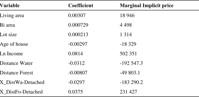
Table 4 Implicit prices

Variable Coefficient Marginal Implicit price

Living area 0.00307 18 946 Bi area 0.000729 4 498 Lot size 0.000213 1 314 Age of house -0.00297 -18 329 Ln Income 0.0814 502 351 Distance Water -0.0312 -192 547.3 Distance Forest -0.00807 -49 803.1 X_DistWa-Detached -0.0297 -183 290.2 X_DistFo-Detached 0.0375 231 427

Running the model with different combinations of the variables shows how robust the model and its variables really are. As can be seen in table 3 the explanatory variables are significant in all versions of the model and have similar coefficients in most cases. Model 3 is the full model and have all variables included. The first model only used explanatory variables and indicates highly significant results. As environmental attributes are added to the model, the explanatory variables are stable. It is only in model 2 that distance to forest variable is positive, however still insignificant. In later models this variable is negative but do have a positive cross-term with detached houses. It is interesting to see that distance to forest is insignificant in all, except the last model where only environmental attributes and income is included.

4.1.1 Estimated coefficients

For most of the estimated coefficients the results are in line with the expectations. The constant term of 14,29 is interpreted as the intercept and is significant at 99% level. The estimated results are in general significant and it is for the environmental attributes that the significance level is

(19)

13 lower or insignificant, the results from these environmental attributes should therefore be handled with caution.

The variable for distance to forest was insignificant and had a surprisingly large p-value (p=0.68). A one-percentage change in distance to forest is expected to have a 0,008% impact on price. It is only with larger changes a great difference in price will be seen. In this model, distance to forest do not have a significant impact on home sales price. One of the cross-term variables, for distance to water and detached house, also showed insignificant results (p=0.105). This p-value is rather close to the 90% significance level, but not close enough to consider the result as significant. 105 observations of 1000 could still be interpreted as a result appeared by chance. The implicit prices estimated with these two variables should be interpreted with caution.

It was rather surprising that the results for the variable for average income was insignificant (p-value 0.11). A number of earlier studied have used neighborhood-dummy-variables (for instance Sander & Haight, 2012), which of many have shown significant results. In this study has average income been used as demographic variable instead of defining neighborhoods, it was however expected to show similar results.

4.2 Distances to natural scenery

Distances to the natural areas are the ones of interest in this study. The variables for distance to forest, lake and the cross-term for house type, all bear important information. The estimated results for all but one variable show negative coefficients, this indicates that decreasing the distance to a natural scenery would increase sales price. Since the model is estimated in log-log form are the numbers interpreted as the percentage change in distance.

The distance to water displayed significant results at the 90% level and indicates that decreasing the distance with 1% would increase sales price with 0.031%. So, a 100-meter decrease in distance from the initial distance 1 km would lead to a 192 547 SEK price increase. This suggests that habitants are willing to pay for the attribute of closeness to water.

The coefficient for distance to forest indicated only a small effect on sales price, were a 1% change in distance responded with a price change of 0.008%. That is, decreasing the distance

(20)

14

from the initial 1 km with 100 meters would increase price with 49 803 SEK. However, the environmental attribute distance to forest, did not show a significant impact on house sales prices.

Instead of the original house-type dummy variable the cross-term for the environmental attributes and detached houses was used. These variables also indicated which impact the distances had on house types and not just the effect of house type alone. The estimated coefficient suggests that a 100-meter decrease to a lake from a detached house, from the initial 1 km, would add an extra 183 290 SEK to the house value. However, this estimation did not show significant results. For forest and detached house the coefficient was positive, which indicates that increasing the distance would increase house sales price. An additional 100-meter to a forest would therefore increase the house price with 231 427 SEK. This would give the net valuation for a 1% change in distance to forest for detached houses of 0.0294%.

4.3 Econometric credibility

The calculated model in table 3 gave a R2 of 0,6537 which implies that the model explains 65% of the variance in prices. This is a relatively high number and indicates that the variables used in the model are reasonably good for estimating the house sales price.

A White’s test was made to see if heteroskedasticity was present. Heteroskedasticity occurs when the assumption of constant variance in the error term is violated and vary along X. The null hypothesis is that the residuals are homoscedastic. A Lagrange multiplier (LM) is calculated, if it exceeds the chi-square critical value then the null is rejected and heteroskedasticity is present. Our calculated LM is 230 and the critical value is 85, we thereby reject the null and accept the alternative that heteroskedasticity is present. This is not good for the credibility of the model and the estimations should be interpreted with caution since the regression is not having minimum variance.

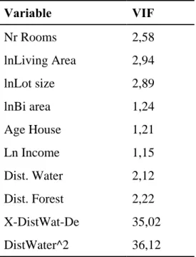
Further credibility tests have been done: the variance inflation factor (VIF) test is one. It is done to indicate if there is multicollinearity between variables, if the VIF is larger than 5, multicollinearity is present (Studenmund 2014). As can be seen in table 5, multicollinearity is present for the cross-term variables. Since these variables move together with distance to the environmental attributes, so it is in some extent anticipated.

(21)

15

Table 5 Variance Inflation factor

Variable VIF Nr Rooms 2,58 lnLiving Area 2,94 lnLot size 2,89 lnBi area 1,24 Age House 1,21 Ln Income 1,15 Dist. Water 2,12 Dist. Forest 2,22 X-DistWat-De 35,02 DistWater^2 36,12

5. Discussion and conclusions

The hedonic model computed for this study showed some overall good results with only a small number of insignificant variables and a R2 of 65% which indicates that a variation in prices can be explained well by the model. The aim of the model was to answer the research question:

- Which impact does closeness to recreational space, such as a lake or nature reserve, have on homes sales prices?

The hypothesis was that a decrease in distance to a natural scenery would increase property price. According to the estimated model and the implicit prices this is to some degree true. Both variables for distances to the lake and forest did show negative coefficients which implies that increasing the distance would have affect house sales price negatively. The model also showed that the value for detached houses near a lake was even higher than for linked or row houses.

Due to the fact that the model was estimated in log-log functional form and that the estimations are presented in percentage change, curves for the implicit prices has not been calculated. This means that by this model we can only tell how a 1% change in an attribute might affect a house’s sales price. The percentage change estimated is assumed to be constant, however the price

(22)

16

change are not constant. Nor has the demand curves been calculated, making the optimum levels for all attributes hard to estimate.

Almost all of the coefficients agree with the previous literature where both Sander and Haight (2012) and Lutzenhiser and Netusil (2001) found results similar to mine. In the later of the two articles, it was found that natural parks had the highest impact on sales price on average and in the first article was a negative coefficient found for distance to a lake and a park. As for my results, the forest variable is a bit surprising since it is a rather small coefficient, have a high risk of appearing by chance and both of these studies had found results where natural areas are valued. It could be that forest areas are easy to come by in the studied neighborhoods and that the value for them are not just found to be that great in this sample.

Comparing my results to Hörnsten and Fredman’s (2000) study, it can be seen that my sample already does have a preferable distance to a forest area and would not have been asked for their WTP for an increased distance, if they had participated in the study. Would this however make my results irrelevant? I do not think so. It is still interesting to find the relationship between a house’s sales price and the distance to a nature, and because of the fact that the coefficient indeed was negative, would make it relevant for valuation of ecosystem services.

As seen detached houses are estimated to experience an additional price increase as the distance to a lake change. This could be to some extent expected since detached houses suggests lower average distance to water in the studied neighborhoods (588 meter versus 763 meters for other house types). Of 104 the observations with less than 400 meters to the lake, 74% were detached houses. These estimations for the cross-terms could tell us one of two things; either that owners of detached houses value proximity to forests less than owners of linked or row houses, or that link or row houses in the study area are more often built near forest areas than detached houses. It could also be a combination of the two statements. Linked and row houses has a similar mean distance to a forest as for detached houses but are however in general sold for less which could make a difference in the estimations.

The estimated results in this study can only be interpreted for this particular studied area and applied on single-family homes. If apartments buildings would had been included in the study, a completely different set of results would had been shown. Apartments also have another kind of pricing. The fact that the neighborhood experiences a higher average income than the rest of

(23)

17 Sweden could also affect the results and the total valuation for all attributes. Distance to city center was not included in this study as it has been in other studies (Sander & Haight 2012 for instance), however average income was included instead as replacement and indicated that sales prices of houses are expected to go up as the buyer’s income is increased.

So, the valuation for the environmental attributes and the ecosystem services in this model are strongly localized. These results show that people in Täby do value the closeness to nature areas. Planners should take this into account when new neighborhoods are planned and built so that both future and present habitants can enjoy the nature and all the benefits that comes with it.

(24)

18

Reference:

Boverket (2019). Typer av ekosystemtjänster. Available:

https://www.boverket.se/sv/PBL-kunskapsbanken/Allmant-om-PBL/teman/ekosystemtjanster/det_har/typer/ Karlskrona:

Boverket (2019-05-16)

Haab, T. C. & McConnell, K.E. (2002). Valuing Environmental and Natural Recourses, the Econometrics of non-market valuation. Cheltenham: Edward Elgar Publishing Limited. Hitta.se (2019). Om livsstilskartan. Available: https://www.hitta.se/livsstil (2019-05-05)

Hörnsten, L. & Fredman, P. (2000). On the distance to recreational forests in Sweden.

Landscape and Urban Planning, vol 51, pp. 1-10.

Lutzenhiser, M., & Netusil, N. R. (2001). The effect of open spaces on a home's sale price. Contemporary Economic Policy, vol. 19, No. 3, pp. 291-298. Available:

http://www.greenstogreen.org/pdfs/resources/resources-openspaces-homesaleprices.pdf

(2019-04-17)

Naturvårdsverket (2019). Naturreservat – vanlig och stark skyddsform. Available:

https://www.naturvardsverket.se/Var-natur/Skyddad-natur/Naturreservat/ (2019-05-27)

Rosen, S. (1974). Hedonic prices and implicit markets: product differentiation in pure competition. Journal of Political Economy, vol. 82, No 1, pp. 34-55

Statistics Sweden (2018). Befolkningsstatisitk: Andra halvåret 2017. Available:

https://www.scb.se/hitta-statistik/statistik-efter-amne/befolkning/befolkningens-

sammansattning/befolkningsstatistik/pong/tabell-och-diagram/kvartals--och-halvarsstatistik--kommun-lan-och-riket/andra-halvaret-2017/ (2019-05-12)

Statistics Sweden (2019a). Inkomster för personer i Sverige. Available:

https://www.scb.se/hitta-statistik/sverige-i-siffror/utbildning-jobb-och-pengar/inkomster-for-personer/ (2019-05-12)

Statistics Sweden (2019b). Sveriges befolkning. Available:

(25)

19 Sander, H.A., Haight, R.G. (2012). Estimating the economic value of cultural ecosystem services in an urbanizing area using hedonic pricing. Journal of Environmental Management, vol. 113, pp. 194-205. Available:

https://www.nrs.fs.fed.us/pubs/jrnl/2012/nrs_2012_sander_001.pdf (2019-04-14)

Stock H.J,, Watson W.M. (2015). Introduction to Econometrics. Third edition. Essex: Pearson Education Limited.

Studenmund, A.H. (2014). Using Econometrics a Practical Guide. 6th ed. Pearson education.

Swedish tax agency (n.d.). Så mäter du ditt småhus. Available:

https://www.skatteverket.se/privat/fastigheterochbostad/fastighetstaxering/deklarerasmahus/m

atreglerforsmahus.4.5cbdbba811c9a768f0c80002011.html (2019-05-16)

Täby kommun (2013). Fakta om Rönningesjön. Available:

https://www.taby.se/globalassets/3.-dokument-per-dokumenttyp/information/trafik--stadsplanering/fakta-om-ronningesjon.pdf (2019-05-11)

Täby Kommun (2019). Motionsspår och friluftsgårdar. Available:

https://www.taby.se/fritid-och-kultur/idrott-och-motion/motionsspar-och-friluftsgardar/ (2019-05-12)

Vatteninformationssystem Sverige (2019). Rönningesjön. Available:

https://viss.lansstyrelsen.se/Waters.aspx?waterMSCD=WA68379026&managementCycleNa

A lake’s impact on suburban dwellings

A lake’s impact on suburban dwellings

– a hedonic price study on housing in Täby

Johanna Berglund

Independent project • 15 credits

A lake´s impact on suburban dwellings

– a hedonic price study on housing in Täby

Acknowledgement

Abstract

Table of Contents

1 Introduction

1.1 Background

1.2 Research question and hypothesis

1.3 Literature Review

2. Theory and methodology

2.1 The hedonic price model

3. Application

3.1 Case study area

3.2 Data

3.3 Variables

4. Results

4.1 The estimation results of the model

4.1.1 Estimated coefficients

4.2 Distances to natural scenery

4.3 Econometric credibility

5. Discussion and conclusions

Reference: