Maximum outer-bank velocity reduction for vane-dike fields installed in channel bends

Maximum outer-bank velocity reduction for vane-dike fields installed in

channel bends

S. Michael Scurlock1, Amanda L. Cox, and Christopher I. Thornton Department of Civil and Environmental Engineering, Colorado State University Drew C. Baird

Sedimentation and River Hydraulics Group, Technical Service Center, Bureau of Reclamation, Denver

Abstract. Hydraulic conditions associated with channel bends in meandering rivers include

secondary, helical currents, mass shift of flow to the outside of the bend, and increased erosion along the outer streambank. Such outer-bank erosion may result in undesired plan-form migration of the stream course, placing valuable land holdings or infrastructure in jeopardy. A type of in-stream transverse rock structure, the vane dike, has been installed in field scenarios to mitigate problematic hydraulics associated with migrating river bends. Flows around vanes and similar structures have been modeled extensively in the past, both physically and numerically, yet, guidelines optimizing key state parameters for the installation of vane dikes in series are still unrealized and application of previous results are generally site specific. Emphasizing the stabilization of the upper reaches of the Middle Rio Grande River below Cochiti Dam, two scaled channel bends were physically modeled with installed vane-dike fields. Structure plan form angle, vertical angle, spacing, and length were altered between testing configurations and comprehensive data collection was performed. The reduction of the outer-bank velocity magnitude was quantified and non-dimensionalized for each tested vane-dike configuration. An approach predicting the outer-bank velocity reduction was developed for collected laboratory data, which approximates vane-dike field velocities for both channel bends with a coefficient of determination of 0.841.

1. Introduction

Flow through channel bends presents a series of important problems facing hydraulic and design engineers. Water surface super-elevation, back currents, vortices, eddies, outer bank erosion and inner bank deposition are all prevalent hydraulic and sediment transport conditions associated with channel bends. Channel bend hydraulics present challenges to both bank stabilization and navigation. Accordingly, in-stream structures have been utilized to redirect current to the channel center and optimize flow conditions to reduce outer-bank velocity. Laboratory and numerical studies have been undertaken (Bhuiyan, et al. 2009; Bhuiyan, et al. 2010; Johnson, et al., 2001, McCoy, et. al., 2008), and some design guidelines developed (Lagasse et al., 1997), However, design guidelines for the geometry and spacing of structures based upon hydraulic and engineering performance are currently limited, and further research into the field of hydraulic structures installed in bends is needed.

In 1975, the completion of the Cochiti Dam on the Rio Grande River resulted in dramatic decrease of sediment delivered to the downstream reach. The downstream reach

1 _{Hydraulics Laboratory, Colorado State University}

1320 Campus Delivery Fort Collins, CO 80523 Tel: (970)491-8757

breached a geomorphic threshold, and the system transitioned from a braiding to meandering regime. To address problematic meandering placing valuable land and

infrastructure at jeopardy, the United States Bureau of Reclamation (Reclamation) initiated a channel maintenance program focusing on the river reach between the downstream side of Cochiti Dam and near Corrales, New Mexico. Vane-dikes, a type of transverse, in-stream stabilization structure, were identified as desirable options for the program because of their inherent habitat advantage over other mitigation approaches such as bank rip-rap; however, the lack of design guidelines associated with the structures presented a concern. Therefore, Reclamation contracted with Colorado State University to construct physical models to investigate hydraulics associated with vane-dike structures installed in channel bends. A trapezoidal channel model was constructed in 2000 to represent generic channel bend types of the Rio Grande reach under scrutiny. The constructed model was evaluated with various weir configurations as detailed by Heintz (2002), Darrow (2004), Schmidt (2005), Kinzli (2005), and Sclafani (2009).

2. Physical modeling

A 1:12 Froude scale model was constructed at the Hydraulics Laboratory at Colorado State University to simulate flow characteristics in a prototype reach of the Rio Grande River. Focusing on the ratio of channel bend radius of curvature to bankfull top width, bends within the prototype were segmented into three classes, Type I with smaller ratio values, Type II with midrange ratio values, and Type III with larger ratio values (Heintz 2002). To bracket prototype plan-form geometries, a generic Type I and Type III bend were selected for evaluation in the physical model. Modeled bend characteristics are detailed in Table 1 and further elaborated upon by Heintz (2002). Vane spacing, plan and profile angle, height, and length were adjusted and hydraulic conditions were evaluated at 8, 12, and 16 cfs, representing prototype values of 66.7, 100.0, and 133.3 percent of bankfull discharge. Velocity fields were evaluated through modeled vane-dike field reaches using an acoustic Doppler velocimeter (ADV). Details regarding model construction, data collection methodologies, and other relevant information relating to vane-dike testing is reported by Heintz (2002), Darrow (2004), and Schmidt (2005). Cumulatively, 130 independent tests were available for data analysis.

Maximum velocities at the outer bank were determined from the filtered,

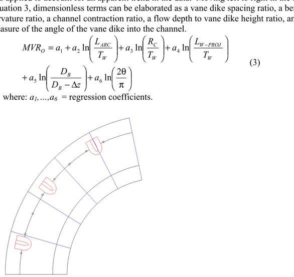
time-averaged velocity vector magnitudes from data obtained by the ADV. Data were collected at locations within the vane dike field as depicted in Figure 1, and the maximum measured velocity magnitude was used for analysis.

3. Maximum velocity ratio approach

Heintz (2002) identified the maximum velocity ratio (MVR) as an important parameter in the quantification of alteration to flow conditions when vane dikes are installed. MVR can be evaluated as the ratio of maximum velocity observed with installed vane dikes to the maximum velocity observed at baseline conditions. For the present analysis, the maximum velocity at the outer bank, or where the vane dike field is installed, is used for comparison to cross-section averaged velocity at baseline conditions. Mathematically, the maximum velocity ratio at the outer bank for the present study was defined as Equation 1.

Baseline Ave

V

MV

MVR

=

where: MVO = maximum velocity magnitude measured along outer bank of channel bend [L/T]; and V_AveBaseline = baseline cross-sectional averaged velocity along thalweg direction

[L/T].

A functional relationship was proposed for MVRO based on independent parameters

identified within the laboratory data as Equation 2.

)

,

,

,

,

,

,

(

Δ

θ

=

f

L

L

R

T

D

z

MVR

where: LW-PROJ = projected length of vane dike into channel [L]; LARC = arc length

(bank-line distance) between center(bank-line of vane dikes [L]; RC = center-line radius of curvature of

channel bend [L]; TW = averaged top width of channel measured at baseline in bend [L];

DB = averaged maximum cross-section baseline flow depth in bend [L]; Δz = difference

between water surface elevation and vane dike crest elevation at baseline conditions [L]; and θ = vane dike plan angle [radians].

From Equation 2, terms were arranged into dimensionless groups, which were

identified to have physically recognizable meanings. A logarithmic form of the equation was applied to account for an apparent trend in the data. Moving left to right in the formed Equation 3, dimensionless terms can be elaborated as a vane dike spacing ratio, a bend curvature ratio, a channel contraction ratio, a flow depth to vane dike height ratio, and a measure of the angle of the vane dike into the channel.

⎟ ⎠ ⎞ ⎜ ⎝ ⎛ π θ + ⎟⎟⎠ ⎞ ⎜⎜⎝ ⎛ Δ − + ⎟⎟⎠ ⎞ ⎜⎜⎝ ⎛ + ⎟⎟⎠ ⎞ ⎜⎜⎝ ⎛ + ⎟⎟⎠ ⎞ ⎜⎜⎝ ⎛ + = − 2 ln ln ln ln ln 6 5 4 3 2 1 a z D D a T L a T R a T L a a MVR B B W PROJ W W C W ARC O (3)

where: a1,…,a6 = regression coefficients.

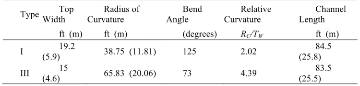
Table 1. Type I and Type III model bend characteristics

Type _Width Top _Curvature Radius of _Angle Bend _Curvature Relative _Length Channel

ft (m) ft (m) (degrees) RC/TW ft (m) I _(5.9) 19.2 38.75 (11.81) 125 2.02 _(25.8) 84.5 III 15 (4.6) 65.83 (20.06) 73 4.39 83.5 (25.5)

4. Results

Statistical analysis software was used to perform backwards linear regression on the natural logarithms of collected data at a statistical significance level of p = 0.05. The statistical procedure begins with the full numerical model and then removes the parameter with the least significance, or highest p-value above a specified level, determined on the basis of an F-distribution. The model ascribes specific p-values to parameters based upon the amount of change generated in the sum of square error, or associated coefficient of determination, when the parameter is either added or removed. Larger p-values correspond to smaller changes in the sum of square error when the parameter is added or removed. The truncated numeric model with the largest p-value term from the previous model removed will produce a new set of p-values for each parameter, and the procedure iterates until all parameters left within the model have associated p-values less than the specified level. A p-value of 0.05 corresponds to a confidence level of 95 percent.

Using the velocity data collected from the physical model, Equation 4 was produced which predicts the Type I and Type III bend MVRO with a coefficient of determinationof

0.655, root mean square deviation of 0.127, and mean error of 34.08 percent.

⎟ ⎠ ⎞ ⎜ ⎝ ⎛ π θ + ⎟⎟⎠ ⎞ ⎜⎜⎝ ⎛ Δ − + ⎟⎟⎠ ⎞ ⎜⎜⎝ ⎛ − ⎟⎟⎠ ⎞ ⎜⎜⎝ ⎛ + − = − 2 ln 149 . 0 ln 186 . 0 ln 779 . 0 ln 276 . 0 791 . 0 z D D T L T L MVR B B W PROJ W W ARC O (4)

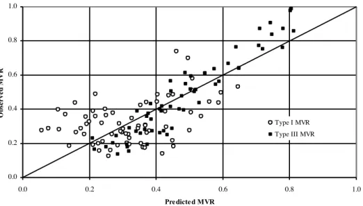
Observed values compared with predicted values from Equation 4 are provided in Figure 2. The term accounting for the difference in radius of curvature between the Type I and Type III bend was not found to be statistically significant.

0.0 0.2 0.4 0.6 0.8 1.0 0.0 0.2 0.4 0.6 0.8 1.0 Predicted MVR Ob se rv ed M V R Type I MVR Type III MVR

Figure 2. Observed vs. predicted values for Equation 4 – Type I and Type III bends identified

When the results of the regression analysis were analyzed, an apparent discontinuity between Type I and Type III bend data was found. Equation 4 predicts the Type III data with a coefficient of determination of 0.910, while Type I data is predicted with a

coefficient of determination of 0.140. Given this discontinuity, Type I and Type III bend data were isolated and regression procedures were rerun for each dataset independently. Equation 5 was produced for Type I data with the only statistically significant

dimensionless term being RC/TW at a 0.05 level, resulting in an coefficient of determination

value of 0.229, root mean square deviation of 0.108, and mean error of 30.90 percent.

⎟⎟⎠ ⎞ ⎜⎜⎝ ⎛ − = W C O T R MVR 1.421 1.136ln (5)

The radius of curvature for each bend is constant and Equation 5 is only a function of channel top width, which is a function of discharge along the entire bend of a prismatic channel. Therefore, the developed relationship for the Type I bend only shows a weak correlation between discharge and maximum velocity along the outer bank.

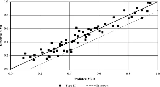
Statistical procedures were executed on the Type III data only, and Equation 6 was developed with a coefficient of determination of 0.918, root mean square deviation of 0.005, and mean error of 15.90 percent.

⎟ ⎠ ⎞ ⎜ ⎝ ⎛ π θ + ⎟⎟⎠ ⎞ ⎜⎜⎝ ⎛ Δ − + ⎟⎟⎠ ⎞ ⎜⎜⎝ ⎛ − ⎟⎟⎠ ⎞ ⎜⎜⎝ ⎛ + − = − 2 ln 206 . 0 ln 289 . 0 ln 044 . 1 ln 2784 . 0 177 . 1 z D D T L T L MVR B B W PROJ W W ARC (6)

Observed versus predicted values for Equation 6 are depicted in Figure 3. The

dimensionless term, RC/TW, was intentionally excluded from Equation 6 as it only accounts

0.0 0.2 0.4 0.6 0.8 1.0 0.0 0.2 0.4 0.6 0.8 1.0 Predicted MVR O b se rve d M V R

Type III Envelope

Figure 3 Observed vs. predicted values for Equation 6 and Equation 7 envelope

To provide a factor of safety, an offset based on the maximum error between observed and predicted MVRO values as computed from Equation 6, excluding outliers identified as

having error greater than two times the root mean square deviation, was added to create an envelope equation. It was found that the maximum error was 0.1329, and application of that offset to Equation 6 produced Equation 7.

⎟ ⎠ ⎞ ⎜ ⎝ ⎛ π θ + ⎟⎟⎠ ⎞ ⎜⎜⎝ ⎛ Δ − + ⎟⎟⎠ ⎞ ⎜⎜⎝ ⎛ − ⎟⎟⎠ ⎞ ⎜⎜⎝ ⎛ + − = − 2 ln 206 . 0 ln 289 . 0 ln 044 . 1 ln 278 . 0 044 . 1 z D D T L T L MVR B B W PROJ W W ARC O (7)

From the analysis performed, it was apparent that a large degree of randomness was observed in the Type I bend maximum velocity ratios that does not appear in the Type III data. The combination of Type I and Type III data for regression analysis was observed to weaken the relationship for the Type III MVRO. However, as illustrated in Figure 2, certain

data within the Type I set appear to coincide with the Type III bends. Type I data were examined to investigate the possibility of identifying data not agreeing with the Type III data. Indicators such as discharge, bend positioning, or number of vane dikes within the bend were not found common amongst outliers. It was hypothesized that the rationale behind the scatter in the Type I bend may be related to the vane-dike geometry, namely vane-dike length and percentage of channel flow area blocked by the structure. For a given radius of curvature over bankfull top width ratio, there may be a limit on percentage flow area blocked or vane-dike length that when breached results in erratic flow patterns that are difficult to describe to the precise level required for maximum velocity reduction ratio prediction. To investigate this possibility, Type I data were analyzed with data segmented by percent of flow area blocked.

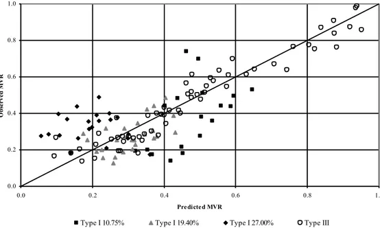
Maximum velocity ratios were identified for the Type I bend as classified by the percent of flow area blocked by the vane dike. Percentage blocked values tested were 10.75, 19.40 or 27.00 percent area blocked. Figure 4 presents the observed versus predicted values of Equation 4 with the Type I bend data segmented according to

percentage area blocked. Datasets pertaining to each percentage area blocked were

incorporated with the Type III data and regression procedures were performed at a p-value of 0.05 using Equation 3. Resulting coefficients of determination for the combined

datasets were 0.885 for the 10.75 percent, 0.888 for the 19.40 percent, and 0.726 for the 27.00 percent. Results of these analyses showed the 10.75 percent and 19.40 percent area blocked MVRO were predicted to a greater degree of accuracy than the 27.00 percent area

blocked data. 0.0 0.2 0.4 0.6 0.8 1.0 0.0 0.2 0.4 0.6 0.8 1.0 Predicted MVR Ob se rv ed M V R

Type I 10.75% Type I 19.40% Type I 27.00% Type III

Figure 4 Observed vs. predicted values for Equation 4 – Type I percent area blocked identified

It was determined that data corresponding to vane dike configurations with 27.00 percent of area blocked were a significant source of error in the numeric model generation for the Type I bend. These data were excluded and the 10.75 and 19.40 percent data were analyzed separately. Starting from Equation 3, and neglecting RC/TW since considering

only one radius of curvature, Equation 8 was generated from backwards regression

procedures at a significance level of 0.05 for the Type I bend data for percent area blocked less than or equal to 19.40 percent.

⎟⎟⎠ ⎞ ⎜⎜⎝ ⎛ Δ − + ⎟⎟⎠ ⎞ ⎜⎜⎝ ⎛ − − = − z D D T L MVR B B W PROJ W O 0.554 0.513ln 0.179ln (8)

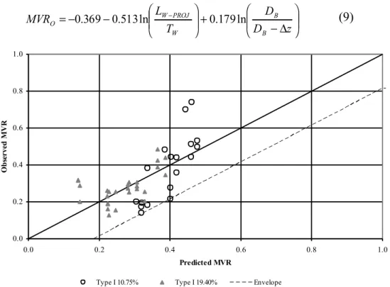
Equation 8 predicts MVR in the Type I bend with a coefficient of determination of 0.446, a root mean square deviation of 0.1036, and mean absolute percent error of 30.25 percent. Observed versus predicted values for Equation 8 are presented in Figure 5. As a factor of safety, the maximum prediction error within two root mean standard deviations was added to Equation 8 to provide an envelope equation. Equation 9 was produced as Equation 8 plus the error offset of 0.1856.

⎟⎟⎠ ⎞ ⎜⎜⎝ ⎛ Δ − + ⎟⎟⎠ ⎞ ⎜⎜⎝ ⎛ − − = − z D D T L MVR B B W PROJ W O 0.369 0.513ln 0.179ln (9) 0.0 0.2 0.4 0.6 0.8 1.0 0.0 0.2 0.4 0.6 0.8 1.0 Predicted MVR O b se rve d M V R

Type I 10.75% Type I 19.40% Envelope

Figure 5 Observed vs. predicted values for Equation 8 and Equation 9 envelope

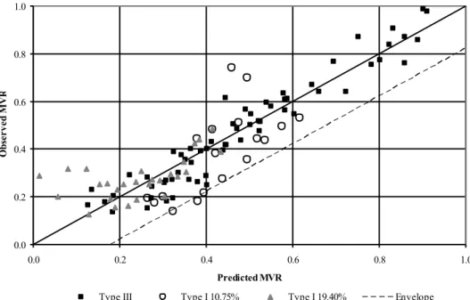
Type I data with percent area blocked values less than or equal to 19.40 percent were combined with that from the Type III bend to optimize the parameters of Equation 3 for both bend types. The resulting Equation 10 predicts MVRO in both bends with a coefficient

of determination of 0.841, a root mean square deviation of 0.091, and mean absolute percent error of 22.15 percent.

⎟ ⎠ ⎞ ⎜ ⎝ ⎛ π θ + ⎟⎟⎠ ⎞ ⎜⎜⎝ ⎛ Δ − + ⎟⎟⎠ ⎞ ⎜⎜⎝ ⎛ − ⎟⎟⎠ ⎞ ⎜⎜⎝ ⎛ + ⎟⎟⎠ ⎞ ⎜⎜⎝ ⎛ + − = − _{0.302 0.166ln} 2 ln 959 . 0 ln 198 . 0 ln 224 . 0 392 . 1 z D D n T L T R T L MVR B B W PROJ W W C W ARC O (10)

Equation 10 predicts Type I bend data with a coefficient of determination of 0.327 and Type III bend data with a coefficient of determination of 0.919. Observed and predicted values for Equation 10 are given in Figure 6.

0.0 0.2 0.4 0.6 0.8 1.0 0.0 0.2 0.4 0.6 0.8 1.0 Predicted MVR Ob se rv ed M V R

Type III Type I 10.75% Type I 19.40% Envelope

Figure 6 Observed vs. predicted values for Equation 10 and Equation 11 envelope

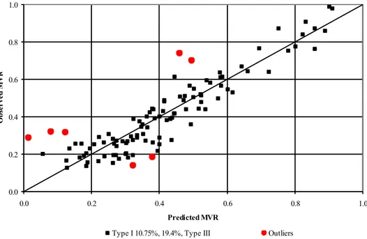
As a factor of safety, an envelope equation was developed to account for the maximum error in the prediction of the outer bank MVRO. Outliers as predicted by Equation 10 were

identified as having an error between observed and predicted values greater than two times the root mean square deviation and are depicted in Figure 7. The maximum offset not including identified outliers was found to be 0.1793, and accordingly, Equation 10 was modified by this amount to produce Equation 11.

⎟ ⎠ ⎞ ⎜ ⎝ ⎛ π θ + ⎟⎟⎠ ⎞ ⎜⎜⎝ ⎛ Δ − + ⎟⎟⎠ ⎞ ⎜⎜⎝ ⎛ − ⎟⎟⎠ ⎞ ⎜⎜⎝ ⎛ + ⎟⎟⎠ ⎞ ⎜⎜⎝ ⎛ + − = − _{0.3018ln 0.166ln} 2 ln 959 . 0 ln 198 . 0 ln 224 . 0 212 . 1 z D D T L T R T L MVR B B W PROJ W W C W ARC O (11)

0.0 0.2 0.4 0.6 0.8 1.0 0.0 0.2 0.4 0.6 0.8 1.0 Predicted MVR Ob se rv ed M V R

Type I 10.75%, 19.4%, Type III Outliers

Figure 7 Observed vs. predicted values for Equation 10 with outlier data identified

5. Conclusions

Analysis was performed on laboratory velocity data and dimensionless relationships were developed for the prediction of the maximum velocity ratio along the outer bank for Type I and Type III channel bends. It was found that relationships developed for Type III bend data were more accurate than those for the comprehensive Type I bend data. Under the assumption that cross-sectional flow area blocked by the vane dikes was significant for a given radius of curvature and top width, three area blocked percentages were separately analyzed within the Type I data. It was found that as the percent area blocked increased, the MVRO became more difficult to predict. Accordingly, the dataset was truncated to

Type I 10.75 and 19.40 percent values, discarding the Type I 27.00 percent dataset which could not be predicted well using the developed empirical relationship, and new regression coefficients were generated.

For Type I bends, Equation 8 is provided as a design guideline for 10.75 and 19.40 percent blockage. Equation 9 may be used to incorporate a factor of safety. For Type III bends, Equation 6 was provided as a guideline for predicting the maximum velocity ratio, and Equation 7 provides an approach with a factor of safety. If a generalized approach is to be used for both bends, or for bends within RC/TW bounds of 2.02 and 4.39, Equation 10

and corresponding Equation 11 with incorporated safety factor were optimized under the Type I percent blockage restrictions. The exact value of percent area blocked where MVRO

prediction is adversely affected for a given RC/TW was not determined. It must be assumed

that percent area blocked be limited to less than approximately 20.00 percent for all RC/TW

values less than 4.39. Percent area blocked was not found to be an influence in Type III bends; however, to ensure applicability of proposed approaches, the value should not exceed 27.00 percent.

Acknowledgements. Funding provided by the Reclamation’s Albuquerque Area Office for

Hydraulic Engineer in the Sedimentation and River Hydraulics Group at Reclamation’s Technical Service Center in Denver Colorado provided review of comments on the paper. Her contribution is also gratefully acknowledged.

References

Bhuiyan, F., Hey, R.D., and Wormleaton, P.R., (2009). “Effects of Vanes and W-Weir on Sediment Transport in Meandering Channels.” Journal of Hydraulic Engineering, Vol. 135, No. 5, May. Bhuiyan, F., Hey, R.D., and Wormleaton, P.R., (2010). “Bank-Attached Vanes for Bank Erosion Control

and Restoration of River Meanders.” Journal of Hydraulic Engineering, Vol. 136, No. 9, Sept.. Heintz, M.L. (2002) “Investigation of Bendway Weir Spacing.” M.S. Thesis, Colorado State University,

Department of Civil Engineering, Fort Collins, CO.

Darrow, J. (2004). “Effects of Bendway Weir Characteristics on Resulting Flow Conditions.” M.S. Thesis, Colorado State University, Department of Civil Engineering, Fort Collins, CO.Johnson, P.A., Hey, R.D., Tessier, M., and Rosgen, D.L., (2001). “Use of Vanes for Control of Scour at Vertical Wall

Abutments.” Journal of Hydraulic Engineering, Vol. 127, No. 9, Sept.

Kinzli, K. (2005). “Effects of Bendway Weir Characteristics on Resulting Eddy and Channel Flow Conditions.” M.S. Thesis, Colorado State University, Department of Civil Engineering, Fort Collins, CO.

Lagasse, P.F., Byars, M.S. Zevenbergen, L.W. and Clopper, P.E., (1997). “Bridge Scour and Stream Instability Countermeaures.” FHWA Rep. HI-97-030, HEC-23, Federal Highway Adminstration, Arlington, Va.

McCoy, A., Constantinescu, G., and Weber, L.J., (2008). “Numerical Investigation of Flow Hydrodynamics in a Channel with a Series of Groynes.” Journal of Hydraulic Engineering, Vol., 134, No. 2

Feb.Schmidt, P. (2005). “Effects of bendway weir field geometric characteristics on channel Flow conditions.” M.S. Thesis, Colorado State University, Department of Civil Engineering, Fort Collins, CO. Sclafani, P. (2009). “Methodology for predicting maximum velocity and shear stress in a sinuous channel

with bendway weirs using 1-D HEC-RAS modeling results.” M.S. Thesis, Colorado State University, Department of Civil Engineering, Fort Colllins, CO