Invited review
Using multi-tracer inference to move beyond
single-catchment ecohydrology
Benjamin W. Abbott
a,⁎
, Viktor Baranov
b, Clara Mendoza-Lera
c, Myrto Nikolakopoulou
d, Astrid Harjung
e,
Tamara Kolbe
f, Mukundh N. Balasubramanian
g, Timothy N. Vaessen
h, Francesco Ciocca
i, Audrey Campeau
j,
Marcus B. Wallin
j, Paul Romeijn
k, Marta Antonelli
l, José Gonçalves
m, Thibault Datry
c, Anniet M. Laverman
a,
Jean-Raynald de Dreuzy
f, David M. Hannah
k, Stefan Krause
k, Carolyn Oldham
n, Gilles Pinay
aa
Université de Rennes 1, OSUR, CNRS, UMR 6553 ECOBIO, Rennes, France b
Leibniz-Institute of Freshwater Ecology and Inland Fisheries, Germany c
Irstea, UR MALY, Centre de Lyon-Villeurbanne, F-69616 Villeurbanne, France dNaturalea, Spain
eUniversity of Barcelona, Spain f
OSUR-Géosciences Rennes, CNRS, UMR 6118, Université de Rennes 1, France g
BioSistemika Ltd., Ljubljana, Slovenia
hCentre d'Estudis Avançats de Blanes, Consejo Superior de Investigaciones Científicas (CEAB-CSIC), Girona, Spain i
Silixa, UK j
Department of Earth Sciences, Uppsala University, Sweden
kSchool of Geography, Earth & Environmental Sciences, University of Birmingham, UK l
LIST - Luxembourg Institute of Science and Technology m
National Institute of Biology, Slovenia n
Civil, Environmental and Mining Engineering, The University of Western Australia, Perth, Australia
a b s t r a c t
a r t i c l e i n f o
Article history: Received 1 April 2016
Received in revised form 18 June 2016 Accepted 23 June 2016
Available online 28 June 2016
Protecting or restoring aquatic ecosystems in the face of growing anthropogenic pressures requires an under-standing of hydrological and biogeochemical functioning across multiple spatial and temporal scales. Recent technological and methodological advances have vastly increased the number and diversity of hydrological, bio-geochemical, and ecological tracers available, providing potentially powerful tools to improve understanding of fundamental problems in ecohydrology, notably: 1. Identifying spatially explicitflowpaths, 2. Quantifying water residence time, and 3. Quantifying and localizing biogeochemical transformation. In this review, we synthesize the history of hydrological and biogeochemical theory, summarize modern tracer methods, and discuss how im-proved understanding offlowpath, residence time, and biogeochemical transformation can help ecohydrology move beyond description of site-specific heterogeneity. We focus on using multiple tracers with contrasting characteristics (crossing proxies) to infer ecosystem functioning across multiple scales. Specifically, we present how crossed proxies could test recent ecohydrological theory, combining the concepts of hotspots and hot mo-ments with the Damköhler number in what we call the HotDam framework.
© 2016 The Authors. Published by Elsevier B.V. This is an open access article under the CC BY-NC-ND license (http://creativecommons.org/licenses/by-nc-nd/4.0/). Keywords: Hydrological tracer Water Environmental hydrology Flowpath Residence time Exposure time Reactive transport GW-SW interactions Hot spots Hot moments Damköhler Péclet HotDam Ecohydrology Crossed proxies Tracer Groundwater Surface water Aquatic ecology ⁎ Corresponding author.
E-mail address:benabbo@gmail.com(B.W. Abbott).
http://dx.doi.org/10.1016/j.earscirev.2016.06.014
0012-8252/© 2016 The Authors. Published by Elsevier B.V. This is an open access article under the CC BY-NC-ND license (http://creativecommons.org/licenses/by-nc-nd/4.0/).
Contents lists available at
ScienceDirect
Earth-Science Reviews
Contents
1. Introduction . . . 20
2. A brief history of theories in ecohydrology and watershed hydrology . . . 21
3. Crossing proxies forflowpath, residence time, and biogeochemical transformation. . . 22
3.1. Water source andflowpath: where does water go when it rains? . . . 23
3.1.1. Water isotopes . . . 23
3.1.2. Solute tracers: pharmaceuticals, ions, dyes, and DOM . . . 25
3.1.3. Particulate tracers: synthetic particles, bacteria, viruses, and invertebrates . . . 27
3.1.4. Heat tracer techniques . . . 28
3.2. Residence time: how long does it stay there? . . . 28
3.2.1. Determining residence time in fast systems . . . 29
3.2.2. Residence time in slow systems . . . 29
3.2.3. Modeling residence time distributions from tracer data . . . 30
3.3. Biogeochemical transformation: what happens along the way? . . . 30
3.3.1. Direct tracers of biogeochemical transformation . . . 31
3.3.2. Indirect tracers of biogeochemical transformation . . . 32
3.3.3. DIC and DOM as tracers and drivers of biogeochemical transformation. . . 32
4. Using crossed proxies to move beyond case studies . . . 33
Acknowledgements . . . 34
References. . . 34
1. Introduction
“The waters of springs taste according to the juice they contain, and they
differ greatly in that respect. There are six kinds of these tastes which the
worker usually observes and examines: there is the salty, the nitrous,
the aluminous, the vitrioline, the sulfurous and the bituminous
…There-fore the industrious and diligent man observes and makes use of these
things and thus contributes to the common welfare.
”
[Georgius Agricola, De Re Metallica (1556)]
The central concerns of ecohydrology can be summarized in three
basic questions: where does water go, how long does it stay, and what
happens along the way (
Fig. 1
). Answering these questions at multiple
spatial and temporal scales is necessary to quantify human impacts on
aquatic ecosystems, evaluate effectiveness of restoration efforts, and
de-tect environmental change (
Kasahara et al., 2009; Krause et al., 2011;
McDonnell and Beven, 2014; Spencer et al., 2015
). Despite a
prolifera-tion of catchment-speci
fic studies, numerical models, and theoretical
frameworks (many of which are detailed and innovative) predicting
biogeochemical and hydrological behavior remains exceedingly dif
fi-cult, largely limiting ecohydrology to single-catchment science
(
Krause et al., 2011; McDonnell et al., 2007; Pinay et al., 2015
).
A major challenge of characterizing watershed functioning is that
many hydrological and biogeochemical processes are not directly
ob-servable due to long timescales or inaccessibility (e.g. groundwater
Fig. 1. Conceptual model of a catchment showing the three basic questions of ecohydrology: where does water go, how long does it stay there, and what happens along the way? Dashed lines represent hydrologicalflowpaths whose color indicates water source and degree of biogeochemical transformation of transported solutes and particulates. The proportion of residence time spent in biogeochemical hot spots where conditions are favorable for a process of interest (McClain et al., 2003) is defined as the exposure time, which determines the retention and removal capacity of the catchment in the HotDam framework (Oldham et al., 2013; Pinay et al., 2015).
circulation or chemical weathering). Consequently, our understanding
of many processes depends on how tightly an intermediate, observable
parameter (i.e. a tracer or proxy) is associated with the phenomenon of
interest. Naturally occurring and injected tracers have been used as
proxies of hydrological, ecological, and biogeochemical processes since
the founding of those
fields (
Dole, 1906; Kaufman and Orlob, 1956
),
and likely since the emergence of thirsty Homo sapiens (
Agricola,
1556
). Methodological advances in ecology, biogeochemistry,
hydrolo-gy, and other
fields including medicine and industry have vastly
in-creased the number of tracers available (
Bertrand et al., 2014
), and
theoretical and computational advances have improved our ability to
interpret these chemical and hydrometric proxy data to infer catchment
functioning and quantify uncertainty (
Beven and Smith, 2015; Davies et
al., 2013; Tetzlaff et al., 2015
). Multi-tracer approaches have been
devel-oped to investigate ecohydrological and biogeochemical functioning
unattainable with single proxies (
Ettay
fi et al., 2012; González-Pinzón
et al., 2013; Urresti-Estala et al., 2015
). Multi-tracer methods provide
tools to address the three fundamental questions in ecohydrology by:
1. Identifying spatially explicit
flowpaths, 2. Determining water
resi-dence time, and 3. Quantifying and localizing biogeochemical
transfor-mation (
Fig. 1
;
Kirchner, 2016a; McDonnell and Beven, 2014; Oldham
et al., 2013; Payn et al., 2008; Pinay et al., 2002
).
While the diversity and number of tracers applied in different
disci-plines provide opportunities (
Krause et al., 2011
), they also represents a
logistical and technological challenge for researchers trying to identify
optimal methods to test their hypotheses or managers trying to assess
ecosystem functioning. Although converging techniques have reduced
the methodological distance between hydrological, biogeochemical,
and ecological approaches (
Frei et al., 2012; Haggerty et al., 2008;
McKnight et al., 2015
), most work remains discipline speci
fic,
particu-larly in regards to theoretical frameworks (
Hrachowitz et al., 2016;
Kirchner, 2016a; McDonnell et al., 2007; Rempe and Dietrich, 2014
).
Furthermore, excitement about what can be measured sometimes
eclipses focus on generating general system understanding or testing
theoretical frameworks to move beyond description of site-speci
fic
het-erogeneity (
Dooge, 1986; McDonnell et al., 2007
).
Several review papers and books have summarized the use of tracers
in quantifying hydrological processes, particularly groundwater-surface
water exchange (
Cook, 2013; Bertrand et al., 2014; Kalbus et al., 2006;
Kendall and McDonnell, 2012; Leibundgut et al., 2011; Lu et al., 2014
).
Here, we expand on this work by exploring how tracers and
combina-tions of tracers (crossed proxies) can reveal ecological, biogeochemical,
and hydrological functioning at multiple scales to test general
ecohydrological theory and to improve ecosystem management and
restoration. Throughout this review we build on an interdisciplinary
theoretical framework proposed by
Oldham et al. (2013)
and
Pinay et
al. (2015)
, which combines the ecological concept of hotspots and hot
moments (
McClain et al., 2003
) with the generalized Damköhler
num-ber (the ratio of transport and reaction times;
Ocampo et al., 2006
) in
what we call the HotDam framework (
Fig. 1
). In
Section 2
, we provide
a brief historical perspective on the development of ecohydrological
theory. In
Section 3
, we explore how crossed proxies can be used to
bet-ter constrain
flowpath, residence time, and biogeochemical
transforma-tion. Finally, in
Section 4
, we discuss how ecological and hydrological
tracer methods can be applied to generate and test hypotheses of
ecohydrological dynamics across scales.
2. A brief history of theories in ecohydrology and watershed
hydrology
Over the past 150 years, numerous frameworks and theories have
been proposed to conceptualize the transport, transformation, and
re-tention of water and elements in coupled terrestrial-aquatic
ecosys-tems. These frameworks are the basis of our current beliefs about
ecohydrological systems and an improved understanding of the
histor-ical context of these ideas could illuminate pathways forward (
Fisher et
al., 2004; McDonnell and Beven, 2014; Pinay et al., 2015
). In this section
we trace the independent beginnings of catchment hydrology and
aquatic ecology in the 19
thand 20
thcenturies followed by a discussion
of how increasing overlap and exchange between these
fields is
contrib-uting to current methodological and conceptual advances.
One of the fundamental goals of catchment hydrology is to quantify
catchment water balance, including accounting for inputs from
precipi-tation, internal redistribution and storage, and outputs via
flow and
evapotranspiration. Early paradigms of catchment hydrology were
fo-cused on large river systems or were limited to single components of
catchment water balance (e.g. non-saturated
flow, in-stream dynamics,
overland
flow;
Darcy, 1856; Horton, 1945; Mulvany, 1851; Sherman,
1932
). Computational advances in the mid-20th century allowed
more complex mathematical models of watershed hydrology, including
the variable source area concept, which replaced the idea of static,
dis-tinct
flowpaths with the concept of a dynamic terrestrial-aquatic
nexus, growing and shrinking based on precipitation inputs and
ante-cedent moisture conditions (
Hewlett and Hibbert, 1967
). Analysis of
catchment hydrographs and water isotopes resolved the apparent
par-adox between the rapid response of stream discharge to changes in
water input (celerity) and the relatively long residence time of stream
water, by demonstrating that most of the water mobilized during
storms is years or even decades old (
Martinec, 1975
). Further modeling
and experimental work investigating heterogeneity in hydraulic
con-ductivity (preferential
flow) and transient storage allowed more
realis-tic simulation of
flowpaths at point and catchment scales, providing a
scaling framework for predicting temporally-variant
flow (
Bencala
and Walters, 1983; Beven and Germann, 1982; McDonnell, 1990
). We
note, however, that characterizing preferential
flow at multiple scales
remains an active subject of research and a major challenge (
Beven
and Germann, 2013
).
Analogous to the hydrological goal of quantifying water balance, a
major focus of ecohydrology is closing elemental budgets, including
ac-counting for inputs from primary production, internal redistribution
due to uptake and mineralization, and outputs via respiration and
later-al export. Early descriptive work gave way to quantitative ecologiclater-al
modelling, using the concept of ecological stoichiometry to link
energet-ic and elemental cycling (
Lotka, 1925; Odum, 1957; Red
field, 1958
).
Work on trophic webs and ecosystem metabolism generated
under-standing of carbon and nutrient pathways within aquatic ecosystems
(
Lindeman, 1942
) and across terrestrial-aquatic boundaries (
Hynes,
1975; Likens and Bormann, 1974
). The nutrient retention hypothesis
re-lated ecosystem nutrient demand to catchment-scale elemental
flux in
the context of disturbance and ecological succession (
Vitousek and
Reiners, 1975
), and experimental watershed studies tested causal
links between hydrology and biogeochemistry such as
evapotranspira-tion and elemental export (
Likens et al., 1970
). A major conceptual
and technical breakthrough was the concept of nutrient spiraling,
which quantitatively linked biogeochemistry with hydrology,
incorpo-rating hydrological transport with nutrient turnover in streams
(
Newbold et al., 1981; Webster and Patten, 1979
). In combination
with the nutrient retention hypothesis, nutrient spiraling allowed
con-sideration of temporal variability on event, seasonal, and interannual
scales for coupled hydrological and biogeochemical dynamics
(
Mulholland et al., 1985
), leading to its application in soil and
ground-water systems (
Wagener et al., 1998
). The telescoping ecosystem
model generalized the concept of nutrient spiraling to include any
ma-terial (e.g. carbon, sediment, organisms), visualizing the stream corridor
as a series of cylindrical vectors with varying connectivity depending on
hydrological conditions and time since disturbance (
Fisher et al., 1998
).
These hydrological and biogeochemical studies helped re-envision the
watershed concept as a temporally dynamic network of vertical, lateral,
and longitudinal exchanges, rather than discrete compartments or
flowpaths.
The 21st century has seen a continuation of the methodological
con-vergence of catchment hydrology and biogeochemistry (
Godsey et al.,
2009; Oldham et al., 2013; Zarnetske et al., 2012
). Speci
fically, two
tech-nological advances have strongly in
fluenced the creation and testing of
ecological and hydrological theory: 1. Hydrological and biogeochemical
models have become vastly more powerful and complex (
Davies et al.,
2013; McDonnell et al., 2007; McDonnell and Beven, 2014
), and 2.
High frequency datasets of hydrological and biogeochemical
parame-ters have come online thanks to advances in remote and environmental
sensors (
Kirchner et al., 2004; Krause et al., 2015; McKnight et al., 2015
).
Increased computing power has allowed the development of
bottom-up, mechanistic models that simulate chemical reactions and water
ex-change based on realistic physics and biology (
Beven and Freer, 2001;
Frei et al., 2012; Trauth et al., 2014; Young, 2003
). At the same time,
more extensive and intensive datasets have allowed the development
of top-down, black-box models based on empirical or theoretical
rela-tionships between catchment characteristics and biogeochemistry
(
Godsey et al., 2010; Jasechko et al., 2016; Kirchner, 2016b
). While
there has been a lively discussion of the merits and drawbacks of
these approaches, developing models that are simultaneously
physical-ly realistic and capable of prediction remains dif
ficult (
Beven and Freer,
2001; Dooge, 1986; Ehret et al., 2014; Kirchner, 2006; Kumar, 2011;
McDonnell et al., 2007
).
Recently, several frameworks have been proposed to integrate
bio-geochemical and hydrological dynamics across temporal and spatial
scales.
Oldham et al. (2013)
and
Pinay et al. (2015)
proposed
comple-mentary frameworks that combine the concept of temporally variable
connectivity (hot spots and hot moments) with the Damköhler ratio
of exposure to reaction times (
Fig. 1
;
Detty and McGuire, 2010;
McClain et al., 2003; Ocampo et al., 2006; Zarnetske et al., 2012
). The
hot spots and hot moments concept is based on the observation that
bi-ological activity is not uniformly distributed in natural systems, but that
transformation tends to occur where convergent
flowpaths bring
to-gether reactants or when isolated catchment compartments become
reconnected hydrologically (
Collins et al., 2014; McClain et al., 2003;
Pringle, 2003
). This concept has been demonstrated in terrestrial and
aquatic ecosystems (
Abbott and Jones, 2015; Harms and Grimm,
2008; Vidon et al., 2010
) and is appealing because using the predicted
or measured frequency of hot spots and hot moments based on
land-scape characteristics allows for more accurate scaling compared to
ex-trapolation of average rates (
Detty and McGuire, 2010; Duncan et al.,
2013
). The generalized Damköhler number estimates the reaction
po-tential of a catchment or sub-catchment component and is de
fined as:
Da
¼
τ
Eτ
Rwhere
τ
Eis the exposure time de
fined as the portion of total
trans-port time when conditions are favorable for a speci
fic process, and τ
Ris a characteristic reaction time for the process of interest (
Oldham et
al., 2013
). When Da
N 1 there can be efficient removal or retention of
the chemical reactant of interest, whereas when Da
b 1, the system is
transport dominated in regards to that reactant (
Fig. 2
). Da varies
sys-tematically with hydrological
flow, approaching infinity in isolated
components when transport is near zero, and typically decreasing
when the ratio of advective transport rate to diffusive transport rate
(the Péclet number) increases (
Oldham et al., 2013
).
The generalized Da represents a scalable metric of biogeochemical
transformation and has been shown to explain variation in the capacity
for catchments or catchment components to remove or retain carbon
and nutrients (
Fig. 3
;
Ocampo et al., 2006; Oldham et al., 2013;
Zarnetske et al., 2012
). Conceptually the hot spots and hot moments
concept is concerned with the
“where” and “when” of hydrological
con-nectivity and biogeochemical activity while Da estimates the
“how
much
” (
Fig. 1
). The HotDam framework combines these concepts in
an effort to provide a realistic and predictive approach to localize and
quantify biogeochemical transformation (
Oldham et al., 2013; Pinay et
al., 2015
). While it is straightforward to understand the relevance of
ex-posure time and connectivity, measuring these parameters in natural
systems can be extremely challenging, requiring the careful use of
mul-tiple tracers. In the following section we outline how tracers can be used
to constrain
flowpath, residence and exposure times, and
biogeochem-ical transformation at multiple scales to generate process knowledge
across multiple catchments.
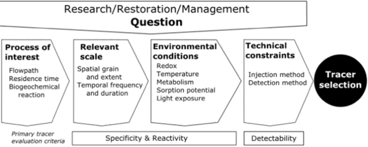
3. Crossing proxies for
flowpath, residence time, and biogeochemical
transformation
Almost any attribute of water (e.g. temperature, isotopic signature,
hydrometric measures such as hydrograph analysis) or material
transported with water (e.g. solutes, particles, organisms) carries
infor-mation about water source, residence time, or biogeochemical
transfor-mation and can be used as a tracer (
Table 1
;
Fig. 4
). Tracers vary in their
speci
ficity (level of detail for the traced process or pathway),
detectabil-ity (limit of detection), and reactivdetectabil-ity (stabildetectabil-ity or durabildetectabil-ity in a given
environment). In practice, there are no truly conservative tracers but
in-stead a gradient or spectrum of reactivity. Tracers can be reactive
bio-logically, chemically, or physically, and all these possible interactions
need to be accounted for when interpreting results. Compounds that
are not used as nutrients or energy sources by biota or which occur at
concentrations in excess of biological demand tend to exhibit less
bio-logical reactivity, though they may still be chemically or physically
reac-tive. Reactivity is contextual temporally and spatially, particularly in
regards to transport through heterogeneous environments typical
of the terrestrial-aquatic gradient. Variations in redox conditions and
elemental stoichiometry mean that the same substance may be
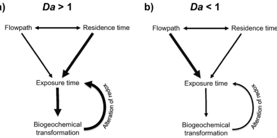
Fig. 2. Schematic relationships between water transport (flowpath and residence time) and biogeochemical processes such as respiration and assimilation when a) Da N 1 (diffusion- or reaction-dominated conditions), and b) Dab 1 (advection- or transport-dominated conditions). Da is the generalized Damköhler number: the ratio of exposure and reaction time scales.
transported conservatively for a portion of its travel time and
non-con-servatively for another. Often, the very reactivity that renders a tracer
unsuitable for conservative duty imparts useful information about
inter-actions and transformations (
Haggerty et al., 2008; Lambert et al.,
2014
). Combining two or more tracers with contrasting properties
(crossing proxies) allows partitioning of multiple processes such as
di-lution and biological uptake (
Covino et al., 2010; Bertrand et al.,
2014
), autotrophic and heterotrophic denitri
fication (
Frey et al., 2014;
Hosono et al., 2014; Pu et al., 2014
), or aerobic and anaerobic production
of dissolved organic matter (DOM; (
Lambert et al., 2014
). The fact that
some tracers are more reactive to certain environmental conditions
means that combining a selectively reactive tracer with a generally
con-servative tracer allows the quanti
fication of exposure time (
Haggerty et
al., 2008; Oldham et al., 2013; Zarnetske et al., 2012
). A
final practical
distinction in tracer methods is between physicochemical signals that
are present within an environment (environmental tracers) and
sub-stances that are added experimentally (injected tracers). Experimentally
added tracers have alternatively been referred to as applied or arti
ficial
tracers (
Leibundgut et al., 2011; Scanlon et al., 2002
), but we refer to
them as injected tracers since many environmental tracers are
anthro-pogenic (arti
ficial).
3.1. Water source and
flowpath: where does water go when it rains?
Besides being one of the existential questions of ecohydrology,
ask-ing where water came from and where it has traveled has direct
impli-cations for management issues including mitigating human impacts on
water quality (
Hornberger et al., 2014; Kirkby, 1987
) and predicting the
movement of nutrients, pollutants, and organisms within and out of the
system (
Chicharo et al., 2015; Hornberger et al., 2014; Mockler et al.,
2015
). The course that water takes through a catchment strongly in
flu-ences residence time and biogeochemical transformation, because
where water goes largely determines how long it stays there and
what sort of biogeochemical conditions it encounters (
Figs. 1, 5
;
Kirkby, 1987
). Flowpaths are in
fluenced by the timing and location of
precipitation in combination with catchment characteristics such as
vegetation, soil structure,
flora and fauna, topography, climate, and
geo-logical conditions (
Baranov et al., 2016; Beven and Germann, 1982;
Blöschl, 2013; Mendoza-Lera and Mutz, 2013
). Depending on the
pur-poses of the study,
flowpaths can be defined conceptually (e.g. surface,
soil, riparian, groundwater) or as spatially-explicitly pathlines
describ-ing individual water masses (
Fig. 5
;
Kolbe et al., 2016; Mulholland,
1993
). Because
flowpaths are temporally dynamic (
Blöschl et al.,
2007; Hornberger et al., 2014; McDonnell, 1990; Strohmeier et al.,
2013
), considering seasonal and event-scale variation in whatever
tracers are being used is essential (
Kirkby, 1987
). Evapotranspiration
is in some ways a special case, as a dominant
flowpath in many
environ-ments, and also as a process that in
fluences flowpaths of residual water,
in
fluencing soil moisture, groundwater circulation, and water table
po-sition (
Ellison and Bishop, 2012; Soulsby et al., 2015
).
3.1.1. Water isotopes
For a tracer to be an effective proxy of
flowpath, it should have high
speci
ficity (sufficient degrees of freedom to capture the number of
con-ceptual or explicit
flowpaths) and low reactivity over the relevant time
period. Perhaps most importantly, it should have similar transport
char-acteristics to water. This is an important consideration because all solute
and particulate tracers have different transport dynamics than water,
particularly when traveling through complex porous media such as
soil, sediment, or bedrock. Even chloride and bromide, the most
com-monly used
“conservative” tracers, can react and be retained by organic
and mineral matrices, sometimes resulting in substantial temporal or
spatial divergence from the water mass they were meant to trace
(
Bastviken et al., 2006; Kung, 1990; Mulder et al., 1990; Nyberg et al.,
1999; Risacher et al., 2006
). Consequently the most effective tracer of
water source and
flowpath is the isotopic signature of the water itself.
Water isotopes have been used to trace storm pulses through
catch-ments (
Gat and Gon
fiantini, 1981
), identify areas of groundwater
up-welling (
Lewicka-Szczebak and J
ędrysek, 2013
), and detect
environmental change such as thawing permafrost (
Abbott et al.,
2015; Lacelle et al., 2014
). Stable and radioactive isotopes of hydrogen
(deuterium and tritium) and oxygen (
16O and
18O) are commonly
used as environmental tracers but have also been injected (
Kendall
and McDonnell, 2012; Nyberg et al., 1999; Rodhe et al., 1996
). The
iso-topic signature of water varies based on type and provenance of
individ-ual storm systems, climatic context (e.g. distance from ocean, elevation,
and latitude), degree of evapotranspiration, and by water source in
gen-eral (e.g. precipitation or groundwater), allowing the separation of
water sources at multiple spatial and temporal scales (
Jasechko et al.,
2016; Kirchner, 2016a; McDonnell et al., 1990; Rozanski et al., 1993
).
While water isotopes can behave conservatively at some
spatiotempo-ral scales and in some environments (
Abbott et al., 2015; Soulsby et
al., 2015
), potential alteration of isotopic signature from evaporation,
chemical reaction, and plant uptake must be accounted for. If water
source and
flowpath can be determined with water isotopes, other
water chemistry parameters can be used to estimate rates of weathering
and biological transformation, or be used as an independent evaluation
of model predictions (
Barthold et al., 2011; McDonnell and Beven,
2014
). Because water isotopes do not have very high speci
ficity
(multi-ple water sources can have the same signature), it is important to
char-acterize site-speci
fic water sources or to cross with another proxy to
appropriately solve mixing equations. The recent development of laser
Fig. 3. Examples of the links between residence time, reaction rate, and exposure time. a) Normalized values of dissolved organic carbon (DOC), dissolved oxygen (DO), isotopic signature, and reactant concentration as water passes through a gravel bar. Reproduced fromZarnetske et al. (2011). b) Modeled prevalence of nitrification and denitrification as a function of the ratio of transit to reaction times (i.e. the Damköhler number; Da). Reproduced fromZarnetske et al. (2012).
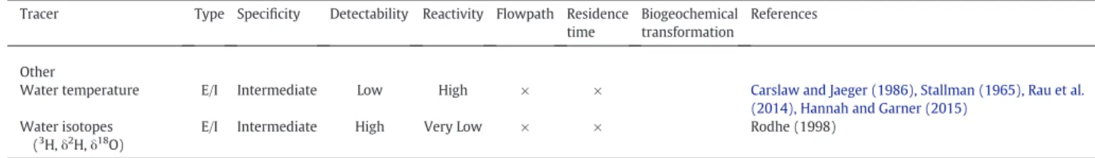
Table 1
List of tracers and their attributes.
Tracer Type Specificity Detectability Reactivity Flowpath Residence
time Biogeochemical transformation References Solute Dissolved gases
Propane I High High volatile × Wallin et al. (2011),Soares et al. (2013)
Chlorofluorocarbons (CFCs)
E/I Intermediate High Low
(CFC-12, 113) Moderate (CFC-11)
× × Lovelock et al. (1973),Thiele and Sarmiento (1990),
Thompson et al. (1974)
Sulfur hexafluoride (SF6) E/I Intermediate High Very Low × Wilson and Mackay (1996)
Radionuclides 3 H,3 He,39 Ar,14 C,234 U, 81 Kr,36 Cl
E/I Intermediate High Low × Solomon et al. (1998), Lu et al. (2014)
Dissolved organic matter (DOM)
E High High High × × Abbott et al. (2014),Quiers et al. (2013),Baker (2005)
δ13 C,δ14
C E/I Intermediate High High × Leith et al. (2014),Raymond and Bauer (2001),Schiff et
al. (1990)
Chemical properties E High High High × × Risse-Buhl et al. (2013)
Optical properties E High High High × Fellman et al. (2010)
Fluorescent dyes Fluorescein,
sodium-fluorescein (uranine)
I High High Low × × Käss et al. (1998),Smart and Laidlaw (1977),
Leibundgut et al. (2009)
Rhodamin WT I High High Low × × Leibundgut et al. (2009), Wilson et al. (1986)
Resazurin I High High High × McNicholl et al. (2007),Haggerty et al. (2008)
Inorganic ions Cl−, Br
-I High High Very Low × Käss et al. (1998), Bero et al. (2016), Frey et al. (2014)
Other anions and cations Rare Earth elements
e.g. Cerium E High High Variable × × Davranche et al. (2005),Dia et al. (2000),Gruau et al.
(2004), Pourret et al. (2009)
Metabolic products, substrates
O2 E High High × × Odum (1957), Mclntire et al. (1964), Demars et al.
(2015)
CO2, DIC E/I High High × Lambert et al. (2014), Wright and Mills (1967)
PO43− E/I High High × Mulholland et al. (1990), Stream Solute Workshop
(1990)
SO42− E/I High High × Hosono et al. (2014)
DOC (e.g. Acetate) E/I Intermediate Intermediate High × × Shaw and McIntosh (1990), Baker et al. (1999)
Stable isotopes δ15 N,δ18 O,δ13 C,δ33 P,δ34
S E/I High High × × Newbold et al. (1981),Sigman et al. (2001), Mulholland
et al. (2009)
Strontium (87 Sr,86
Sr) E Intermediate Intermediate Very Low × Graustein (1989),Wang et al. (1998)
Particulate Artificial sweeteners
Acersulfame-K, sucralose E High High Very Low × Buerge et al. (2009),Lubick (2009),Scheurer et al.
(2009)
Pharmaceuticals drugs Carbamazepine,
sulfamethoxazole, and diclofenac, caffeine, triclosan, and naproxen
E High High High × Arvai et al. (2014),Lubick (2009),Riml et al. (2013),
Andreozzi et al. (2002),Clara et al. (2004),Kurissery et al. (2012),Durán-Álvarez et al. (2012),Buerge et al. (2003),Liu et al. (2014),Chefetz et al. (2008)
Particles
Chaff, nano-particles, clay, kaolinite,fluorescent microspheres
I High High variable × Davis et al. (1980), Packman et al. (2000a, 2000b),
Arnon et al. (2010)
Synthetic DNA (coated or naked)
I High High Low × Foppen et al. (2013),Mahler et al. (1998),Sharma et al. (2012)
Particulate organic matter (POM)
E/I Intermediate High variable × × × Newbold et al. (2005), Trimmer et al. (2012),
Drummond et al. (2014)
Macroinvertebrates E Intermediate High × × × Dole-Olivier and Marmonier (1992), Marmonier et al.
(1992),Capderrey et al. (2013),Blinn et al. (2004)
Terrestrial diatoms E High High Moderate × Pfister et al. (2009), Klaus et al. (2015), Tauro et al.
(2015),Klaus et al. (2015), Naicheng Wu et al. (2014), Coles et al. (2015)
Bacteria
Fecal coliforms E High High Moderate × Leclerc et al. (2001), Stapleton et al. (2007), Characklis
et al. (2005), Weaver et al. (2013)
Non coliforms E High High Moderate × × Bakermans et al. (2002), Bakermans and Madsen
(2002), Jeon et al. (2003)
Virus
Pathogens E High High High × × Harwood et al. (2014), Updyke et al. (2015)
Bacteriophages E High High High × × Keswick et al. (1982), Rossi et al. (1998), Goldscheider
spectrometers has substantially decreased the cost of water isotope
analysis, opening up new possibilities for spatially extensive or high
fre-quency measurements (
Jasechko et al., 2016; Lis et al., 2008; McDonnell
and Beven, 2014
).
3.1.2. Solute tracers: pharmaceuticals, ions, dyes, and DOM
While solutes are typically more reactive and have different
trans-port dynamics from the water that carries them, the sheer number of
different species that can be measured allows for great speci
ficity in
de-termining water
flowpaths. A wide variety of solutes including natural
ions, anthropogenic pollutants,
fluorescent dyes, and dissolved carbon
have been used as environmental tracers to determine water source
and
flowpath (
Hoeg et al., 2000; Kendall and McDonnell, 2012
). Solute
concentrations and isotopic signatures can convey complementary
in-formation, for example strontium (Sr) concentration can distinguish
surface and subsurface water, while the
87Sr/
86Sr ratio which varies
be-tween bedrock formations, can reveal regional provenance (
Ettay
fi et
al., 2012; Graustein, 1989; Wang et al., 1998
). When many solute
concentrations are available, correlated parameters are often combined
into principal components before determining water sources via end
member mixing analysis (
Christophersen and Hooper, 1992
). While
end member mixing analysis is widely used and provides
straightfor-ward estimates of conceptual
flowpaths, it is sensitive to the assignment
of end members, the selection of tracers, and the assumption of
conser-vancy in solute behavior (
Barthold et al., 2011
). As always, using
multi-ple tracers of different types (e.g. stable isotopes and solutes) results in
more robust and reliable mixing models (
Bauer et al., 2001
).
Pharmaceuticals and other synthetic compounds have contaminated
most aquatic environments and are increasingly being used to trace
ag-ricultural and urban wastewater sources and
flowpaths (
Durán-Álvarez
et al., 2012; Liu et al., 2014; Roose-Amsaleg and Laverman, 2015;
Stumpf et al., 1999; Ternes, 1998; Tixier et al., 2003
). Analyses for
many of these compounds have become routine due to emerging
con-cern for human and ecosystem health, bringing down costs and
improv-ing detectability (
Andreozzi et al., 2002; Clara et al., 2004; Kurissery et
al., 2012
). Many of these compounds are bioactive or adsorb to
Fig. 4. A variety of ecohydrological tracers organized by temporal and spatial scale. The range of scales reported in the literature for each tracer or group of tracers is indicated by the bars with the points representing the typical or most common scales of use. Shading represents fundamental ecohydrological question (where does water go, how long does it stay, and what happens along the way) and shape represents tracer type.
Table 1 (continued)
Tracer Type Specificity Detectability Reactivity Flowpath Residence
time
Biogeochemical transformation
References
Other
Water temperature E/I Intermediate Low High × × Carslaw and Jaeger (1986), Stallman (1965), Rau et al.
(2014), Hannah and Garner (2015)
Water isotopes (3
H,δ2 H,δ18
O)
sediment (e.g. caffeine, triclosan, and naproxen), limiting most
applica-tions to small temporal and spatial scales (
Buerge et al., 2003; Chefetz et
al., 2008; Durán-Álvarez et al., 2012
). However, arti
ficial sweeteners
(e.g. acesulfame-K and sucralose) and some drug compounds (e.g.
car-bamazepine, sulfamethoxazole, and diclofenac) appear to be resistant
to degradation for several weeks under a range of conditions and
could be used as biomarkers of human activity (
Arvai et al., 2014;
Buerge et al., 2009; Lubick, 2009; Riml et al., 2013; Scheurer et al.,
2009
). The biodegradability of some pharmaceuticals (e.g. tetracycline)
decreases with redox potential (
Cetecioglu et al., 2013
), meaning their
concentration relative to more resistant compounds could be used to
quantify anoxia, though to our knowledge this approach has not yet
been used.
In addition to environmental tracers that are already present in a
system, experimentally injected solutes have long been used to quantify
flowpath and water source. Synthetic fluorescent dyes such as
fluores-cein have been used since the end of the 19th century and are still
wide-ly used today to test connectivity and water transfer (
Flury and Wai,
2003; Smart and Laidlaw, 1977
). Fluorescent dyes express a range of
re-activity and offer outstanding detectability and speci
ficity, with some
dyes such as
fluorescein and rhodamine WT detectable at
concentra-tions in the parts per trillion range (
Turner et al., 1994
). Most dyes
suitable for duty as
flowpath tracers have sulfonic acid groups and are
synthesized from sodium salts to increase solubility in water (
Cai and
Stark, 1997; Leibundgut et al., 2011
). Emission wavelengths are
charac-teristic for each dye, making it possible to combine multiple dyes with
different properties (
Haggerty et al., 2008; Lemke et al., 2014
).
Draw-backs to
fluorescent dyes include a relatively small number of suitable
dyes (less than ten families), sensitivity to pH and temperature,
adsorp-tion to sediment, and relatively high cost depending on how much dye
is needed (
Leibundgut et al., 2011
).
Dissolved carbon compounds are some of the most versatile solute
tracers and also some of the most complex. Unlike the single-compound
tracers discussed above, DOM consist of thousands of different
com-pounds with distinct properties (
Cole et al., 2007; Zsolnay, 2003
) and
turnover times that can vary from minutes to millennia (
Abbott et al.,
2014; Catalá et al., 2015; Hansell and Carlson, 2001
). DOM chemical
composition, isotopic signature, optical properties, and stoichiometry
constitute a highly detailed signature or
fingerprint that can be used
to determine water source and
flowpath (
Clark and Fritz, 1997;
Schaub and Alewell, 2009
). Using multiple DOM characteristics allows
DOM to effectively be crossed with itself, e.g. simultaneously
determin-ing
flowpath, residence time, and biogeochemical transformation
(
Chasar et al., 2000; Helton et al., 2015; Palmer et al., 2001; Raymond
Fig. 5. Hierarchical spatial scales from an ecohydrological perspective for various catchment components. Relevant physical and ecological controls onflowpath, residence time, and biogeochemical reaction often change with scale, requiring the use of tracers with different characteristics. Adapted fromFrissell et al. (1986).
and Bauer, 2001
). While DOM has incredible speci
ficity, it is the primary
food and nutrient source for microbial food webs and is therefore highly
reactive (
Evans and Thomas, 2016; Jansen et al., 2014
). Nonetheless, at
the catchment scale, DOM concentration is often assumed to be
conser-vative and is regularly included with other solutes to determine water
source in end member mixing analysis (
Larouche et al., 2015; Morel et
al., 2009; Striegl et al., 2005; Voss et al., 2015
). Stable and radioactive
carbon isotopes of DOM, particulate organic matter (POM), and
dis-solved inorganic carbon (DIC) have been used to distinguish surface
water from groundwater as well as determine connectivity between
terrestrial and aquatic environments (
Doucett et al., 1996; Farquhar
and Richards, 1984; Marwick et al., 2015
). Because the
δ
13C of dissolved
carbon derived from algae and terrestrial plants differs in some
environ-ments,
δ
13C of dissolved carbon can be used to separate terrestrial and
aquatic water and carbon sources (
Fig. 6
;
Mayorga et al., 2005;
Myrttinen et al., 2015; Rosenfeld and Roff, 1992; Tamooh et al., 2013;
Telmer and Veizer, 1999
). The
Δ
14C of DOM and POM, an indicator of
time since
fixation from the atmosphere, has been used to separate
depth of
flowpaths (e.g. modern surface soil carbon versus deeper,
older sources) and also as a general indicator of agricultural and urban
disturbance (
Adams et al., 2015; Butman et al., 2014; Vonk et al., 2010
).
There are many methods to characterize DOM molecular
composi-tion (e.g. exclusion chromatography, nuclear magnetic resonance,
ther-mally assisted hydrolysis and methylation-gas chromatography-mass
spectrometry, and Fourier transform infrared spectroscopy-mass
spec-trometry) and optical properties (e.g. ultraviolet-visible absorption
spectra and
fluorescence spectroscopy;
Jaffé et al., 2012; Jeanneau et
al., 2014; Spencer et al., 2015
). Often the post-processing of these
mea-surements is as technically involved as the meamea-surements themselves
(
Chen et al., 2003; Jaffé et al., 2008; Stedmon and Bro, 2008
), and
interpreting the ecological relevance of the outputs of these analyses
re-mains a major challenge and area of active research (
Fellman et al.,
2009; Huguet et al., 2009; Spencer et al., 2015; Zsolnay, 2003
).
Conse-quently, analyses of DOM composition and optical properties are often
most useful when paired with
field or laboratory assays of DOM
reactiv-ity or biodegradabilreactiv-ity (
McDowell et al., 2006; Vonk et al., 2015
). The
re-cent development of
field-deployable fluorometers and spectrometers
has allowed real-time monitoring of DOM characteristics to determine
changes in water source and
flowpath (
Baldwin and Valo, 2015;
Downing et al., 2009; Fellman et al., 2010; Khamis et al., 2015;
Sandford et al., 2010; Saraceno et al., 2009
). For example total
fluores-cence has been used to trace in
filtration of surface water into karst
systems and protein-like
fluorescence has been used as an indicator of
fecal bacteria and DOM biodegradability (
Balcarczyk et al., 2009;
Baldwin and Valo, 2015; Quiers et al., 2013
). Excitation-emission
matri-ces of DOM (
Chen et al., 2003
) have been used to trace land
fill leaching
into rivers, with signals detectable at dilutions of 100
–1000 fold,
sug-gesting this detection method is fast and cost-effective for river
man-agers and water quality regulators (
Baker, 2005; Harun et al., 2015,
2016
).
3.1.3. Particulate tracers: synthetic particles, bacteria, viruses, and
invertebrates
Particulate tracers such as chaff and sediment have been used for
thousands of years to make invisible
flowpaths visible (
Davis et al.,
1980
). Bacteria were
first used to trace water source before the advent
of germ theory when John Snow traced the London Broad Street cholera
outbreak to sewage-contaminated water from the Thames and local
cesspits (
Snow, 1855
). More recently, a wide range of particles
includ-ing biomolecules, viral particles, bacteria, bio
films, diatoms, colloids,
and macroinvertebrates have been implemented to trace
flow and
water source (
Capderrey et al., 2013; Foppen et al., 2013;
Mendoza-Lera et al., 2016; Rossi et al., 1998
). Particles can have
ex-tremely high speci
ficity and detectability and have been used in a
vari-ety of environments including
flowing surface waters, lakes,
groundwater, and marine environments (
Ben Maamar et al., 2015;
Garneau et al., 2009; Harvey and Ryan, 2004; Vega et al., 2003
). While
particles travel through complex media differently than the water that
moves them, this is an advantage when the goal is to trace particulate
transport such as sediment or POM. Because POM is an important
car-bon and nutrient source in aquatic ecosystems (
Pace et al., 2004;
Vannote et al., 1980
), tracing its transport and accumulation provides
insight into the development of hot spots and moments (
Drummond
et al., 2014; Vidon et al., 2010
); see
Section 3.3
).
Bacteria are the most common particulate tracer, with fecal
coli-forms routinely used to identify human contamination of water sources
(
Leclerc et al., 2001
). The purposeful use of bacteria as tracers began
with an antibiotic-resistant strain of the bacterium Serratia indica
which was readily assayed by its bright red colonies on nutrient agar
media (
Ormerod, 1964
). Subsequent applications combined actively
re-producing Serratia indica with dormant Bacillus subtilis spores that
be-haved as conservative tracers, to model dispersion and transit times of
a
field of sewage discharge to a coastal zone (
Pike et al., 1969
). Starting
in the 1970s, improved imaging techniques allowed viruses, particularly
bacteriophages, to be used as tracers of groundwater and ocean
circula-tion (
Hunt et al., 2014
). Because of their small size, high host-speci
ficity,
low cost of detection, and resistant physical structure, bacteriophages
tend to perform better than bacteria or yeasts, particularly in
groundwa-ter applications (
Rossi et al., 1998; Wimpenny et al., 1972
), suggesting
that bacteriophages could
fill an important gap in the current
hydroge-ology toolbox. Improvements in quantitative polymerase chain reaction
techniques and biosynthesis technologies have lowered costs of
bacteri-al and virbacteri-al anbacteri-alyses and opened the way for a new generation of high
speci
ficity, high detectability tracers.
Still smaller than bacteriophages, environmental and synthetic DNA
(eDNA and sDNA, respectively) have extremely high speci
ficity and
de-tectability and relatively low reactivity (
Deiner and Altermatt, 2014;
Foppen et al., 2013
). While extracellular eDNA has primarily been
used for species detection in freshwater environments (
Ficetola et al.,
2008; Vorkapic et al., 2016
), it also has potential as a hydrologic tracer,
with eDNA from lacustrine invertebrates used to trace lake water up to
10 km from its source (
Deiner and Altermatt, 2014
). Tracer sDNA is
pro-duced by automatic oligonucleotide synthesis and is normally short
(less than 100 nucleotides), which allows approximately limitless
unique sequences (4 nucleotides
100= 1.61 × 10
60). Stop codons
distin-guish the sDNA from eDNA, and injected sDNA is analyzed by
quantita-tive polymerase chain reaction with custom primers. sDNA has been
used to trace sediment transport when bound with montmorillonite
Fig. 6. A meta-analysis including unpublished data ofδ13
C values observed in streams and rivers across the globe for dissolved inorganic carbon (DIC), particulate inorganic carbon (PIC), dissolved organic carbon (DOC), and dissolved CO2. Note that mostly C3plant dominated catchments are included.
clay (
Mahler et al., 1998
) and in combination with magnetic
nano-par-ticles (e.g. polylactic acid microspheres and paramagnetic iron
parti-cles) to enhance recoverability and durability in the environment
(
Sharma et al., 2012
). Though high tracer losses (50 to 90%) can occur
immediately after injection, the remaining sDNA shows transport
dy-namics similar to chloride or bromide and is stable for weeks to months
(
Foppen et al., 2011, 2013; Sharma et al., 2012
).
Diatoms (eukaryotic microalgae; 2
–500 μm) have long been used as
indicators of water quality (
Rushforth and Merkley, 1988
) and more
re-cently as tracers of
flowpath (
P
fister et al., 2009
). The timing and
abun-dance of the arrival of terrestrial diatoms to the stream channel can
indicate the source of storm
flow and the extent and duration of
hydro-logic connectivity across the hillslope-riparian-stream continuum
(
P
fister et al., 2009
). Because some terrestrial diatoms are associated
with certain landscape positions or land-use types, this tracer has high
speci
ficity, though sample analysis requires substantial expertise
(
Martínez-Carreras et al., 2015; Naicheng Wu et al., 2014
). The
possibil-ity of using quantitative polymerase chain reaction techniques to
auto-mate diatom identi
fication and quantification could increase the
availability and applications of this approach.
Finally, macroinvertebrates (aquatic insects, crustaceans, mollusks,
and worms) have been used as indicators of ecosystem health and to
delineate surface and groundwater
flowpaths (
Boulton et al., 1998;
Marmonier et al., 1993
). The presence or absence of individual
macroin-vertebrate species can be used to identify zones of hyporheic exchange
as well as to distinguish upwelling from down welling zones both at the
bedform and reach scales (
Blinn et al., 2004; Capderrey et al., 2013;
Dole-Olivier and Marmonier, 1992
). For example, the presence of
stygobiont species (i.e. species living exclusively in groundwater) in
the hyporheic zone is indicative of strong upwelling patterns (
Boulton
and Stanley, 1996
).
3.1.4. Heat tracer techniques
Water temperature is an extremely reactive tracer with low speci
fic-ity and detectabilfic-ity that has nevertheless been widely used to identify
water source and
flowpath by exploiting thermal differences in
ground-water, surface ground-water, and precipitation (
Anderson, 2005; Constantz,
2008; Hannah et al., 2008; Krause et al., 2014
). Similar to water isotopes,
heat is a property of the water itself, rather than a solute or particle.
However, unlike isotopes, thermal signature is very rarely conservative
over long distances or times. Heat is an effective tracer at
ecohydrological interfaces where it has been used to predict the
behav-ior of aquatic organisms in streams (
Ebersole et al., 2001, 2003;
Torgersen et al., 1999
) and to understand the impact of
groundwater-surface water exchange
flows on catchment-scale biogeochemical
bud-gets (
Brunke and Gonser, 1997; Krause et al., 2011; Woessner, 2000
).
Until recently, the thermal resolution of most temperature sensors has
been quite low and temperature data has been limited to point
mea-surements. The development of distributed temperature sensing
(DTS) was a watershed moment for heat tracers since DTS allows
large-scale,
fine resolution temperature measurements. DTS takes
ad-vantage of temperature-sensitive properties of standard or specialized
fiber optic cable to quantify temperature along the length of the cable
(
Selker et al., 2006a; Tyler et al., 2009; Westhoff et al., 2007
). Because
cable can be deployed in any con
figuration, DTS allows quantification
of vertical, lateral, and longitudinal
flowpaths and fluxes. Cables in
river-beds have been used to detect spatial variability of groundwater
dis-charge and redis-charge (
Lowry et al., 2007; Mamer and Lowry, 2013;
Mwakanyamale et al., 2012; Selker et al., 2006b
), identify and model
lat-eral in
flows (
Boughton et al., 2012; Westhoff et al., 2007
), and assess the
role of solar radiation and riparian vegetation shading on stream heat
exchange (
Boughton et al., 2012; Petrides et al., 2011
). Cable can be
wrapped around poles to increase spatial resolution and installed in
streambeds to monitor vertical hyporheic and groundwater
flowpaths
(
Briggs et al., 2012; Lautz, 2012; Vogt et al., 2010
). With
“active” DTS,
heat pulses can be sent along the length of the cable to determine
thermal conductivity of the soil and water matrix (
Ciocca et al., 2012
).
In combination with solute or particulate proxies, heat could be a
sensi-tive tracer of changes in water source during storm events and of how
much and how fast water moves between different compartments of
the catchment.
Another technological breakthrough in heat tracing was the
devel-opment of thermal imagery techniques that can remotely measure
sur-face and shallow subsursur-face water temperatures from satellites,
airborne platforms, or on the ground (e.g.
Cherkauer et al., 2005;
Deitchman and Loheide, 2009; Durán-Alarcón et al., 2015; Jensen et
al., 2012; Lalot et al., 2015; Lewandowski et al., 2013; P
fister et al.,
2010; Schuetz and Weiler, 2011
; Stefan
Kern et al., 2009; Wawrzyniak
et al., 2013
). Though quanti
fication of thermal images remains
challeng-ing, thermal imaging is a valuable complement to other tracers of
flowpath and water source because it makes intersecting water masses
visible at ecohydrological interfaces. It has proven effective in
character-izing in-stream
flowpaths, lateral water exchanges, groundwater
in-puts, and distribution of thermal refugia (
Dugdale et al., 2015; Jensen
et al., 2012; Johnson et al., 2008; Lewandowski et al., 2013; P
fister et
al., 2010
).
3.2. Residence time: how long does it stay there?
Where water goes is closely connected to how long it stays there.
Water residence time is a key parameter that in
fluences hydrology,
bio-geochemistry, and ecology at the catchment scale and within different
catchment components (
Fig. 5
;
Kirchner, 2016b
). Because residence
time is directly proportional to the volume of water, it is also important
for management of water resources (
Collon et al., 2000; Scanlon et al.,
2002
). Compared with the in
finite variety of potential water sources
and
flowpaths, residence time is satisfyingly straightforward. It is
de-fined as the amount of time a mass of water stays in a domain of interest
(e.g. catchment, reach, bedform;
Fig. 4
) and can mathematically be
de-scribed as pool size (amount of water) divided by the rate of in
flow
(input residence time) or out
flow (output residence time), or as the
dis-tribution of water ages in the domain of interest (storage residence
time;
Davies and Beven, 2015
). The similarity or divergence of these
three parameters of residence time depends on spatiotemporal scale
and changes in storage, which can alter interpretation of modeling
and tracer estimates of residence time (
Botter et al., 2010; Rinaldo et
al., 2011
). The simplest and most common metric of residence time is
the mean residence time, but for many practical problems (e.g.
predic-tion of contaminant propagapredic-tion or removal) it is desirable to know
the residence time distribution or transit time distribution, which can
be modelled based on environmental or injected tracer data (
Eriksson,
1971; Gilmore et al., 2016; McGuire and McDonnell, 2006; Stream
Solute Workshop, 1990
). Because residence time is de
fined by the
cho-sen spatial realm, it is inherently scalable across point, hillslope,
catch-ment, and landscape scales (
Fig. 5
;
Asano et al., 2002; Maloszewski
and Zuber, 1993; Michel, 2004; Poulsen et al., 2015; Vaché and
McDonnell, 2006
), though the relative in
fluence of antecedent storage,
celerity, and the ratio of new to old water on residence time varies
with scale (
Davies and Beven, 2015
).
Residence time is central to the HotDam framework because it is
necessary to calculate rates of biogeochemical transformation and
be-cause the amount of time water, solutes, and particulates spend in
dif-ferent catchment components can determine the location and
duration of hot spots (
McClain et al., 2003; Oldham et al., 2013; Pinay
et al., 2015
). Residence time at event and seasonal scales is commonly
modeled based on hydrograph analysis. While this method has been
very effective at predicting water discharge, it cannot separate young
and old out
flow due to the celerity problem (see
Section 2
) and
there-fore cannot reliably determine residence time on its own (
Clark et al.,
2011; McDonnell and Beven, 2014
). Tracer methods in conjunction
with hydrometric analysis can overcome this problem by determining
flowpath (
Martinec, 1975; Poulsen et al., 2015; Tetzlaff et al., 2015
) or
water age directly (
Gilmore et al., 2016; Rodhe et al., 1996
). Techniques
for determining residence time have been reviewed in great detail
else-where (
Darling et al., 2012; Fontes, 1992; Foster, 2007; Hauer and
Lamberti, 2011; Kendall and McDonnell, 2012; Kirchner, 2016b; Payn
et al., 2008; Plummer and Friedman, 1999; Scanlon et al., 2002
), so in
this section we will focus on how crossed-proxy methods could be
brought to bear to quantify and reduce uncertainty, organized by spatial
and temporal scale.
3.2.1. Determining residence time in fast systems
For rapid-transit systems with residence times on the order of
mi-nutes to months (e.g. bedforms, river networks, shallow soils, and
small lakes), most methods of measuring residence time use injected
tracers (
Bencala and Walters, 1983; Stream Solute Workshop, 1990
).
All methods for determining residence time by tracer injection work
on the same basic principle. Assuming that a tracer has the same
trans-port dynamics as water, its rate of dilution after injection is protrans-portional
to the renewal time of a system. Mean residence time and the
distribu-tion of residence times can be calculated from the overall rate of
disap-pearance and the change in removal rate over time, respectively (
Payn
et al., 2008; Schmadel et al., 2016; Wlostowski et al., 2013
).
Conserva-tive behavior of the selected proxy is therefore paramount, since
remov-al by any processes other than dilution and advection (e.g. biologicremov-al,
chemical, or physical reactivity) will directly bias the estimate of
resi-dence time (
Nyberg et al., 1999; Ward et al., 2013
). Tracers can be
added instantaneously or at a known, constant rate depending on the
size of the system and the desired level of detail for the distribution of
residence times (
Payn et al., 2008; Rodhe et al., 1996; Wlostowski et
al., 2013
). For surface water systems (e.g. streams), tracer concentration
is measured at a downstream sampling point, and for subsurface
sys-tems, tracer propagation can be monitored via wells (
Zarnetske et al.,
2011
) or electric resistance tomography for electrically conductive
tracers such as salts (
González-Pinzón et al., 2015; Kemna et al., 2002;
Pinay et al., 1998, 2009
). The shape of the breakthrough curve (the
change in tracer concentration over time at the sampling point)
repre-sents the distribution of residence times. Adequate sampling of the tail
of the break through curve is important to capture slower
flowpaths
and because
flowpaths with residence times longer than the arbitrary
duration of the monitoring will be missed (
González-Pinzón et al.,
2015; Schmadel et al., 2016; Ward et al., 2013
). Tracers with high
de-tectability that can be monitored continuously (e.g.
fluorescent dyes
or sodium) are particularly well suited to determine residence time.
There is a huge diversity of more or less conservative tracers that have
been used to determine short-term residence time including
isotopical-ly labelled water (
Nyberg et al., 1999; Rodhe et al., 1996
), solutes such as
chloride, bromide, and
fluorescent dyes (
González-Pinzón et al., 2013;
Payn et al., 2008
), dissolved gases such as propane, sulfur hexa
fluoride
(SF6), and chloro
fluorocarbons (CFCs;
Molénat et al., 2013; Soares et
al., 2013; Thompson et al., 1974; Wallin et al., 2011
), particulates like
sDNA, viral particles, and nanoparticles (
Foppen et al., 2011, 2013;
Hunt et al., 2014; Ptak et al., 2004; Sharma et al., 2012
), and even hot
water (
Rau et al., 2014
).
For systems with residence time greater than a few days but less
than a year (e.g. hillslopes, headwater catchments, and the
non-saturat-ed zone), hydrometric methods such as mass balance or hydrograph
de-composition are often used to estimate residence time (
Kirchner,
2016b; McDonnell and Beven, 2014; Poulsen et al., 2015
). For systems
with available background chemistry data, it is possible to directly
trace residence time using variation in system inputs (i.e. precipitation
or upstream in
flow). Typically the isotopic or chemical signature of
pre-cipitation or in
flow over time is compared with the signature of system
out
flow (
McGuire et al., 2002; Peralta-Tapia et al., 2015; Rodhe et al.,
1996; Stewart and McDonnell, 1991; Stute et al., 1997
). The integrated
discharge and timing of the arrival of the distinct water mass in different
system components allows the calculation of reservoir size and
resi-dence time.
3.2.2. Residence time in slow systems
For systems with residence times longer than a year, injected tracer
methods are obviously not practical due to time constraints, not to
men-tion the inordinate mass of tracer that would need to be injected into
the system. For slow systems, a variety of environmental tracer methods
have been used including historical or current anthropogenic pollution,
naturally occurring geochemical tracers, and known paleo conditions
(
Aquilina et al., 2012, 2015; Böhlke and Denver, 1995; Kendall and
McDonnell, 2012; Plummer and Friedman, 1999; Schlosser et al., 1988
).
For
“young” groundwater less than 50 years old, radioactive tritium
(
3H) from aboveground nuclear testing in the 60s and 70s, radioactive
krypton (
85Kr) produced during reprocessing of nuclear rods, and
CFCs and SF6 from manufacturing have been used to determine the
time since a water parcel was last in contact with the atmosphere
(
Fig. 7
; (
Ayraud et al., 2008; Leibundgut et al., 2011; Lu et al., 2014
).
Dat-ing with these tracers relies on comparDat-ing the concentration in the
groundwater sample with known historical atmospheric concentrations
after applying a solubility constant based on recharge temperature and
atmospheric partial pressure.
3H and
85Kr have half-lives (t
1/2
) of 12.3
and 10.8 years, respectively, meaning an additional correction must be
applied to back calculate initial concentration. The ratio of
3H to
3He
(the radioactive decay product of
3H) is often used to achieve greater
certainty and precision in this correction (
Schlosser et al., 1988
).
3H is
attractive as a tracer because it recombines with water and therefore
has the same transport dynamics, though drawbacks include its short
window of production and uneven global distribution (
Fig. 7
b). As
noble gases,
85Kr and
3He are biochemically highly conservative, but
dis-persion and degassing can complicate interpretation. Until recently,
large sampling volumes (
N1000 L) were needed for
85Kr and other
ra-dionuclide analyses. The development of atom trap trace analysis
(ATTA) and advanced gas extraction techniques are bringing these
vol-umes down, though sampling procedures are still non-negligible (
Lu et
al., 2014
). CFCs are synthetic organic compounds that were used in
Fig. 7. Atmospheric concentrations of a) chlorofluorocarbons (CFCs) and sulfur hexafluoride (SF6) produced for refrigeration and insolation, and b) tritium (3H) and 85
Kr produced from nuclear testing and rod reprocessing. Data fromAhlswede et al. (2013)and water.usgs.gov/lab/software/air_curve