STATISTICAL STUDY OF THEEARTH'S MAGNETOPAUSEBOUNDARY LAYER PARTICLEPOPULATIONS

(1)

DEGREE PROJECT, IN ENGINEERING PHYSICS , SECOND LEVEL STOCKHOLM, SWEDEN 2015

STATISTICAL STUDY OF THE

EARTH'S MAGNETOPAUSE

BOUNDARY LAYER PARTICLE

POPULATIONS

TIMOTHÉE ACHILLI

KTH ROYAL INSTITUTE OF TECHNOLOGY

(2)

2015-07-24

STATISTICAL STUDY OF THE EARTH’S

MAGNETOPAUSE BOUNDARY LAYER

PARTICLE POPULATIONS

MASTER THESIS REPORT

D

EGREE

P

ROJECT IN

S

PACE

P

HYSICS

–

EF226X

TIMOTHÉE ACHILLI

SUPERVISORS: CHRISTIAN JACQUEY & BENOIT LAVRAUD

(3)

2

ABSTRACT

While double ion populations, with a cold population originating from the solar wind and a hotter one from the magnetosphere, are frequently observed in the Earth’s low-latitude boundary layers, similar double electron populations are seldom recorded. We performed a statistical study of ion and electron double populations near the magnetopause by using 7 years of THEMIS particle data. After a preliminary study of magnetopause crossings characteristics, in particular by determining the typical energies of ion and electron populations in regions near the magnetopause, we set up an automated detection algorithm for identifying regions with combined ion and electron double populations.

The statistical study carried out with respect to IMF conditions in the upstream solar wind during and just before the events suggests that such combined ion and electron Double Population Boundary Layers (DPBL) form preferentially under northward IMF but with a significant BY component.

We interpret this trend as a result of reconnection of the same magnetosheath field line in both hemispheres, but with at least one end reconnecting in its hemisphere at lower latitude with a closed magnetospheric field line which already contains a hot electron source.

(4)

3

INTRODUCTION

The processes that regulate the interaction between the solar wind and the Earth’s magnetosphere are still matter of significant debate. In 1930 Chapman and Ferraro [1] first proposed the idea that the Earth’s strong magnetic field would hold off the solar wind plasma, creating a cavity within which it would be confined. The pressures of the Earth’s magnetic field and the solar wind are in overall equilibrium, with the magnetosphere shrinking when the solar wind pressure increases, and expanding when it decreases. The magnetopause, which is the outer boundary of the magnetosphere, is a thin sheet of electric current separating this solar wind plasma from the geomagnetic field, again as Chapman and Ferraro first proposed. This magnetopause, separating plasma of solar and magnetospheric origins, was originally viewed as impermeable (figure 1).

Figure 1: Cross section of a simple model of the magnetosphere in the noon-midnight meridian (from Kivelsson & Russel, 1995)

In both the solar wind and the magnetosphere, particles can flow freely along magnetic field lines. But as dictated by the frozen-in-flux concept, particles can only mix only along flux tubes, never across them. This explains well observed particles flows in both the solar wind and the magnetosphere, but not the nature of the interaction between them. Dungey proposed an explanation in 1961[2]:

According to a now generally accepted paradigm, the particle and energy flow inside the magnetosphere is largely driven by magnetic reconnection occurring at different locations on the magnetopause, as a function of the solar wind properties and in particular the Interplanetary Magnetic Field (IMF) orientation.

(6)

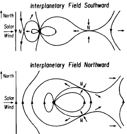
5 If we assume the IMF is directed southward, that is to say antiparallel to the geomagnetic field on the front of the magnetosphere, then reconnection occurs at the sub-solar magnetopause (figure 2, upper panel).

When the IMF is directed northward, by contrast, anti-parallel field lines from the solar wind and the magnetosheath reconnect at high latitudes poleward of the Earth’s magnetic cusps, as has been supported by observations [3][4][5]. The reconnected field lines would convect sunward and then eventually tailward, away from the reconnection site (figure 2, lower panel).

Figure 2 : Sketch of the field lines in the noon-midnight meridian for the two cases when the interplanetary magnetic field is antiparallel to the magnetic field near the nose of the magnetosphere (top) and when it is parallel (bottom)

Magnetic reconnection is a process that can only happen if the criterion of frozen-in-flux breaks down. It is known to be particularly frequent at the magnetopause. Antiparallel field lines, separated by a thin current sheet, are cut and reconnected (figure 3). Plasmas originally from two different regions thus find themselves on the same flux tube and are therefore able to mix on the newly formed field lines.

(7)

6

Figure 3: Basic X-line reconnection picture. Plasma and magnetic field flow in from the top and bottom of the figure and flow out toward the sides.

The reconnection process at the sub-solar magnetopause under southward IMF creates large-scale topological changes, with newly open field lines connecting the solar wind plasma to the Earth’s ionosphere. This opening allow solar wind particles to flow through the magnetopause, thereby driving momentum transport into the magnetosphere and the triggering of significant geomagnetic activity. This entry of plasma leads to the formation of boundary layers just inside the magnetopause. Under southward IMF, these boundary layers observed at low latitudes on the dayside are directly explained by reconnection in the nearby sub-solar region. However, it is not fully clear why these boundary layers are also observed under northward IMF. Several processes have been brought up to explain their formation, with varying success: (1) particle diffusion through waves-particle interaction, which may not explain boundary layers thicker than0.5RE, (2) the Kelvin-Helmholtz instability, which may not explain their formation in the sub-solar region owing to the lack of velocity shear there (basic ingredient of the KH-instability), and (3) double high-latitude reconnection.

This latter possibility for dayside boundary layers formation under northward IMF implies a double reconnection process of the same magnetosheath field lines in both the southern and northern lobes. This process would create newly closed field lines, almost instantaneously, with trapped, dense plasma of solar origin [6][7].

Indeed the observations of a population of dense and stagnant ions during extended periods of northward IMF [8], mixed with a population of magnetospheric ions in the low latitude boundary layers, could account for this theory. The dense ion population could be magnetosheath ions from solar wind origin that would have been trapped on the newly reconnected field lines after the double reconnection.

Low absolute parallel heat fluxes in the boundary layers present on the sunward side of the magnetopause under northward IMF, which result from the presence of bidirectional heated electrons, have also been reported [9]. These bidirectional electrons can be interpreted as the signature of newly closed magnetosheath field lines that have reconnected in the high latitude magnetopause, tailward of the cusp, in both hemispheres.

(8)

7 The magnetopause boundary layer thus typically contains a cold electron population and a cold ion population, both of solar origin, as well as a hot ion population of magnetospheric origin. The presence of a hot electron population of magnetospheric origin is, however, seldom observed. Such cases have been reported [10][11] but no statistical studies have been carried out. It is the objective of this internship to perform a comprehensive statistical study of their occurrence to determine what physical process may explain the rare presence of hot electrons in dayside magnetopause boundary layers.

For that purpose we will look for regions where we observe a double peak in fluxes at energies typical of the magnetosheath and magnetosphere, for both ions and electrons. From now on we refer to these as the Double Population Boundary Layer (DPBL).

(9)

8

1. METHODOLOGY AND RESULTS

1.1. INSTRUMENT

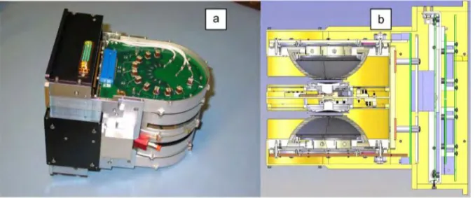
Our study is mainly based on the analysis of the ESA instrument onboard the 5 THEMIS spacecraft [13]. This plasma instrument consists of a pair of top-hat electrostatic analyzers (ESAs) that measure ion and electron energy per charge (E/q). Figure 4 shows a picture (a) and cross-section (b) of the sensors which are packaged together. With the spin of the satellite, both heads cover 4π steradians. The sensors have selectable energy sweeps (programmable starting energy with logarithmic or linear sweep steps) and are generally swept in energy (logarithmically) from ~32 keV for electrons and ~25 keV for ions, down to ~6-7 eV. Nominal operations have 32 sweeps per spin, with 31 energy samples per sweep, plus one sample energy retrace, resulting in a typical measurement resolution with a ΔE/E ~ 32%. Particle events are registered by microchannel plate (MCP) detectors.

Figure 4: Picture (a) and cross-section (b) of the ESA instrument.

The principle of the top-hat electrostatic analyzer is illustrated in Figure 5. For example, for the electron instrument, a positive voltage is applied in the internal half-sphere while the external one remains at the ground. The resulting electric field locally orthogonal to the half spheres deflects the electron trajectory so that only the particles with a particular energy are able to reach the detector.

E = R/ΔR*V/2, where E is the particle energy, R the median radius of the hemisphere, ΔR the difference between the radius of both hemispheres and V the applied voltage).

The detectors are microchannel plates which consist of plate of glass hollowed by inclined microscopic channels and chemically treated in such a way that an incident particle impact produces an avalanche of electrons.

(10)

9

Figure 5: Illustration of the top-hat electrostatic analyzer principle.

1.2. OIEROSET CASE STUDY

We present here an overview of the event studied by Oieroset et al. [10] in 2008 with the aim of illustrating a well-established case of DPBL.

On 2007/06/03 the THEMIS spacecraft “encountered an extended region of

nearly-stagnant magnetosheath plasma attached to the magnetopause on closed field lines.”

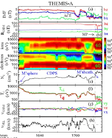
Below is the event crossing recorded by THEMIS-A. There is a zone of mixed population of both magnetospheric and heated magnetosheath ions between the magnetosphere and the magnetosheath, lasting for more than half an hour. In this region, density and temperature are intermediate between magnetospheric and magnetosheath values.

(11)

10

Figure 6: Event crossing recorded by THEMIS A. (a) Time-shifted IMF measured by ACE. (b–h) TH-A measurements of the magnetic field, ion and electron energy spectrograms (in eV/(cm2-s-sr-eV)), ion density, temperature and velocity, and the M component of the velocity tangential to the magnetopause and perpendicular to the magnetic field, respectively. The horizontal dark blue bar in (c) marks the CDPS region. The light blue bar in (d) denotes the region of mixed magnetosheath and magnetospheric electrons (from Oieroset et al. [10]).

In addition to these ion populations, we note the presence of mixed population of both magnetospheric and heated magnetosheath electrons with well-balanced field-aligned and anti field-field-aligned fluxes (figure 7).

Figure 7: THEMIS A electron pitch-angle distribution measured in the mixed electron region of the CDPS.

(12)

11 In the outer portion of the boundary layer where only heated magnetosheath electron populations where present, field-aligned and anti-field-aligned electron fluxes were also well balanced, which means that the entire boundary layer was on closed field lines. The key unknown here, and which is only alluded in past works (including [10]), is why hot electrons are seen in only parts of the boundary layer, and why so rarely overall.

Several processes will be considered to explain the presence of hot magnetospheric electrons and the formation of such DPBL: on the basis of the present case study, these are:

1) Local diffusion (wave-particle interactions)

Unlikely because for this case there was a very smooth magnetic field with no significant -wave activity during and in the vicinity of DPBL observations.

2) Local entry through KH-instability

Unlikely because no boundary waves were observed and no large velocity shear is observed nor expected at this location.

3) Diffusive entry or KH further downtail, followed by sunward convection along the magnetopause.

Unlikely because this would not result in a thin (0,9RE) boundary layer attached to the magnetopause on the dayside, and furthermore no sunward flow was observed in the DPBL.

4) Capture of magnetosheath plasma by poleward-of-cusp reconnection in both hemisphere.

Possible. It can explain the presence of counter-streaming and heated magnetosheath electrons on the boundary layer field lines, but it does not explain the presence of hot ions and electrons. The presence of hot ions has often been related to gradient and curvature drift from the tail towards the dusk LLBL where mixed ions populations are often observed [12], but this process should allow a similar mixing process on the dawn side (owing to oppositely directed gradient and curvature drift for electrons) while mixed electrons are rarely observed, even on the dawn side (as we will further demonstrate later).

5) Another possibility is the capture of magnetosheath plasma onto closed field lines by reconnection tailward of the cusp in one hemisphere and equatorward of the cusp in the other hemisphere with previously closed field lines.

Indeed, for purely northward IMF and reconnection in the lobes tailward of both cusps, the newly closed field lines are only expected to contain ions and electrons of

(13)

12 magnetosheath energies (slightly heated). This is because lobe field lines are typically empty of any plasma. An efficient way of mixing plasma of solar origin with both hot ions and electrons of magnetospheric origin would, however, be to reconnect at least one end of the IMF field line with a field line that was previously closed and filled with magnetospheric plasma. This may be done if there is a sufficient Y-component in the IMF orientation so that an IMF field line may reconnect in the lobe in one hemisphere but more on the side of the magnetosphere and at lower latitude in the other hemisphere with a previously closed field line (already containing a source of hot magnetospheric ions and electrons). The present case study (Oieroset) is consistent with this hypothesis since the IMF By is around 4 nT and the Clock angle is varying between 30° and 70°.

In section 2 we investigate the statistical properties of the DPBL to obtain better insights into its driving conditions and possible origin.

1.3. STATISTICAL CHARACTERISTICS OF ION AND ELECTRON POPULATIONS IN REGIONS SURROUNDING THE MAGNETOPAUSE

We performed a statistical analysis of the omnidirectional ion and electron fluxes measured by the ESA instruments (Electrostatic Analyser [13]) onboard the 5 THEMIS spacecraft as they flew around the magnetopause. This study provides a global picture of typical ion and electron spectra in the magnetopause boundary layer with respect to the location in the magnetosphere. It will allow us in the next sections to determine the relevant criteria for identifying the DPBL with the help of automated data-mining.

For this statistical study we used all available THEMIS data in the mode "FULL" at 96 second time resolution. The periods covered are:

 2007/04/01 to 2014/07/24 for THEMIS A, D, and E

 2007/04/01 to 2009/12/30 for THEMIS B and C, that is, until they became ARTEMIS in early 2010 and were sent into orbit around the moon.

SET-UP OF THE MAGNETOPAUSE CROSSINGS DATABASE

We first processed an automated detection algorithm for magnetopause crossings and then represented the ion and electron spectra with respect to a transition

parameter [14] used as a proxy of the spacecraft location relative to the

magnetopause.

We know that in the magnetosphere, the particle density is low and temperature is high, while conversely on the other side of the magnetopause, in the magnetosheath, the plasma is dense and cold. Thus the ratio of the density over the temperature is a

(14)

13 relevant and often used proxy for detecting the magnetopause. In our study, we used the ratio n/T where n is the ion density and T the ion temperature (

, the ion anisotropy is negligible for such analysis). Both n and T are obtained from the ESA measurements.

The first step of magnetopause crossing automated detection has been performed through the analysis of changes in the n/T transition parameter. A candidate was identified and recorded when absolute values of the transition parameter change at the scale of 5 minutes exceeded some threshold. Five minutes was found to be a good compromise between magnetopause oscillation time (we want to look at effective magnetopause crossing and not all quick and often multiple crossings when the magnetopause position oscillates past the spacecraft) and data resolution.

The threshold used for changes in n/T has been fixed after looking at a large number of magnetopause crossings and chosen high enough so that only unambiguous magnetopause crossings events are retained. For our purpose, losing some events is not detrimental as long as statistics remains sufficient and representative.

Figure 8: Example of a magnetopause crossing obtained from the AMDA tool. (a) Ion spectrogram. (b) Electron spectrogram. (c) Magnetic field in GSE coordinates. (d) n/T (in cm-3 /eV). (e) Δ(n/T) (in cm-3 /eV).

(15)

14 The criteria we used for magnetopause identification are the following:

 Δ(n/T)5min = |n/T(t) – n/T(t-5 min)| > 0.08 cm-3 /eV

 7 RE < R < 15 RE where R is the geocentric distance of the satellite

 xGSE > -2 RE

Visual examination of some cases and their spatial distribution revealed that the collection of events obtained included some bow shock crossings. A second step was devised with the inclusion of an additional criterion to eliminate bow shock crossings. After having compared the variations of various parameters, the ion temperature was chosen as the additional parameter in our algorithm to get rid of bow shocks. Indeed, changes in temperatures are systematically and significantly larger through the magnetopause than through the bow shock.

After having examined a large number of bow shock and magnetopause crossings we settled the following threshold (figure 9):

 Δ(T)5min = |T(t) – T(t-5 min)| > 500 eV

Figure 9: Bow shocks (in red) and magnetopauses (in blue) distribution in the X-RYZ

plane.

.

We note that there are some points inside of the magnetosphere that have been eliminated by our criterion, which are unlikely bow shocks this close to Earth. This could be plasma from the plasmasphere that have first been detected as magnetopause crossings because of the associated large change in ion density,

(16)

15 implying a large change in n/T. But the change in T is not large enough to meet our second criterion, which thus turns out to remove both spurious bow shock and plasmasphere crossings.

This full data mining permits us to obtain a catalog of magnetopause crossings, of which we plotted the locations in figure 10.

Figure 10: Plot of the magnetopause crossings. The color bar indicates the solar wind ram pressure (in cm-3) as the satellite crosses the magnetopause.

Figure 10 shows, as expected from mere pressure equilibrium arguments, that when the solar wind pressure is high the magnetopause is statistically closer to Earth. For this representation the solar wind ram pressure comes from the OMNI database, which gathers data from several solar wind monitor satellites (ACE, Geotail, Wind, …) time-shifted to the bow shock. We must also note that there is an orbital artefact at a radius of ~11 RE because most of the data come from THEMIS A, D, and E, which have a perigee of 11RE. This explains the lower density of points in Figure 10 beyond 11 RE.

AVERAGE CHARACTERISTICS OF THE ION AND ELECTRON

POPULATIONS AROUND THE MAGNETOPAUSE

The magnetopause crossing database we have constituted contains a large number of events; we decided to divide the dataset in 7 regional areas going from the nose of the magnetosphere to its flanks (figure 11). Each region has a large number of samples, thereby permitting a statistical study. Based on this we now present a large-scale picture of the typical ion and electron spectrograms through the magnetopause (as a function of the transition parameter) in different regions of the magnetopause.

(17)

16

Figure 11: Splitting of the magnetosphere in 7 areas that include all the magnetopause crossings.

We used energy flux data in reduced mode from the ESA instrument. This mode is omnidirectional but has a high time resolution (3s). It includes 6 sub-modes corresponding to different energy ranges. The first step consisted in identifying the sub-modes inside the data and standardizing them into a unique mode.

All the magnetopause crossings from our catalogue have been extended by 1 hour (30 minutes before the magnetopause crossing and 30 minutes after) and all particle spectra where averaged with a 1-minute time resolution. The data have then been superimposed by binning them with respect to n/T (the transition parameter [14]), separately for each of the 7 sectors and for 4 IMF orientations (north, south, dawn and dusk).

As shown in past works [14], the magnetopause transition parameter is a way of ordering magnetopause data to resolve ambiguities in the sequence of satellite data, caused especially by the motion of the boundary. The data have been represented as a spectrogram for each sector: for all IMF conditions we plot the mean energy fluxes as a function of the transition parameter and the particle energy in figures 12a & b.

(18)

17

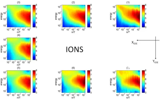
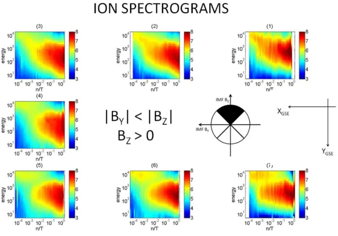
Figure 12a: Ion spectrograms for each of the 7 areas (on the right side the nose of the magnetosphere and on the left side the flanks). The color bar indicates the energy flux in power of ten. (1)-(7) Zones as shown in Figure 11.

Figure 12b: Electron spectrograms for each of the 7 areas (on the right side the nose of the magnetosphere and on the left side the flanks). The color bar indicates the energy flux in power of ten. (1)-(7) Zones as shown in Figure 11.

(19)

18 The transition parameter organizes very well the mean spectra in the different regions surrounding the magnetopause. We clearly see the magnetosheath population for high n/T and the magnetosphere for low n/T. For ions, in figure 12a, we notice the presence of a double ion population on the dusk flank of the magnetosphere and on the nose for n/T values ranging from 10-2 cm-3 /eV to 10-3 cm -3

/eV. This mixing does not exist on the dawn flank, which supports the hypothesis that the hot ions we observe may originate from the tail and would have (gradient and curvature) drifted to the dusk side.

By contrast, on figure 12b, the average spectrograms show that double populations are much rarer for electrons. It is somewhat seen in the nose sector (figure 12b-4) for a small range of n/T around 10-3 cm-3 /eV, as well as on the two adjacent sectors (figure 12b-3&5), but is totally absent in other areas.

We also proceeded the same way after separating data according to 4 IMF orientation conditions in the Y-Z (GSE) plane, which is known as primary parameter for ordering boundary layer and magnetopause characteristics. After splitting the data according to IMF By and BZ values we drew the same ion and electron spectrograms in figures 13 & 14.

(20)

19

Figure 13a: Ion spectrograms for northward IMF and |BY| < |BZ|.

(21)

20

Figure 13c: Ion spectrograms for low BZ and positive BY.

(22)

21

Figure 14a: Electron spectrograms for northward IMF and |BY| < |BZ|.

(23)

22

Figure 14c: Electrons spectrograms for low BZ and positive BY.

(24)

23 We should first highlight here that such statistical displays naturally create a smooth transition in the spectra which is not representative of any given magnetopause crossing, where transitions are typically more abrupt. It may also spuriously create double populations (separated in energy) if in the same n/T bin one averages low density cold populations with high density hot populations, for example. Nevertheless, on average the presence of double peaks in either ions or electrons should be related to a higher likelihood of observing such double populations in the associated region.

We will not focus on all the details of these plots, but note two main characteristics of interest for our purpose. From the average ion spectra, we first see that when the IMF is directed northward (Figure 13-a), the double population in the dusk side is much more visible than when the IMF is southward (Figure 13-b). These are also observed for large IMF BY. For electrons, we also notice that the double population is more visible for northward and strong IMF BY. Typically, the double populations in electrons are mostly seen on the dayside and not on the flanks. In particular there is no obvious double population at dawn that would constitute the counterpart of the observed double ion populations at dusk, given the opposite gradient and curvature drift from the tail for electrons. These trends will be examined in further details in the discussion section.

Thanks to these spectrograms we could determine the characteristic ion and electron energies to take into account for the automated search of the DPBL.

2. DOUBLE POPULATION BOUNDARY LAYER (DPBL)

2.1. SELECTION CRITERIA

DPBLs have been sought with the data mining permitted by the AMDA tool for the same periods as the magnetopause analysis of the previous section.

For processing and download time purposes, the data mining sampling has been performed on 1-minute averaged data (originally with a 3-second time resolution) retrieved from the ESA instruments. Taking into account the results reported in the previous section, the search criteria have been built based on ion and electron energy fluxes in particular energy bands and distance from Earth. The energy bands we have chosen (3 for ions and 4 for electrons) are given in Table 1.

The commonly observed magnetopause boundary layers include three populations: cold ions and electrons coming from the magnetosheath, and hot ions of magnetospheric origin. More rarely, an additional population of hot electrons can be observed (cf. Section 2). The aim of the present analysis is to determine its spatial

(25)

24 distribution and occurrence, and how it is ordered by interplanetary conditions (IMF). Using the AMDA data-mining functionality we tracked the events when a double population is concurrently found in both ions and electrons. To do this we have set requirements on the energy fluxes averaged on the energy bands of each population. The tests are:

 Ion double population: o I1 & I3 > 105

eV/(cm2-s-sr-eV) o I2/I1 & I2/I3 < 90%

 Electron double population: o E1 > 105

eV/(cm2-s-sr-eV) & E4 > 106 eV/(cm2-s-sr-eV) o E2/E1 & E2/E4 & E3/E4 < 90%

I1 I2 I3 E1 E2 E3 E4

Table 1: Energy channels chosen for the DPBL search. We call I1..3 and E1..4 the averaged energy fluxes on the energy bands of the population in the corresponding

column.

This data mining search finds a lot of time intervals that present a double peak a, but a lot of them are 1-minute in duration, which is the data mining sampling time. Since the original resolution is 3 seconds, many such cases may come from a time-aliasing process; i.e., a double peak profile may come from the averaging of magnetosheath and magnetosphere particle fluxes which may not be mixed if looking at higher time resolutions (below the 1 minute averaging). For this reason we remove all 1 minute intervals from our analysis (even if we do not free ourselves from the same problem if the magnetopause is oscillating during more than 1 minute, which is in any case rarer).

(26)

25 Figure 15 confirms that the energy channels we chose fit very well the actual peaks and holes in energy flux of the DPBL populations. Figure 16 confirms that the energy flux threshold was also well defined. We should have detected most of the events.

Figure 15: Spectra of all the DPBL events (every grey line is an instantaneous spectrum at 1-minute resolution). The boxes are the energy ranges for each population and “holes” that we have chosen

Figure 16: Flux thresholds (eV/(cm2-s-sr-eV)) for each populations of ions (top) and electrons (bottom).

(27)

26

2.2. LOCATION AND OCCURRENCE OF THE DPBL

Here we first visualize the spatial distribution of the DPBL (figure 17) and then analyse the difference in the distribution along the X-axis between all magnetopause crossings and the DPBL events (figure 18).

Figure 17: Map of DPBL events location.

(28)

27 We first notice in Figure 17 a slight dawn-dusk asymmetry in the DPBL observations, but in reality this comes from an orbital bias as there are in fact the same asymmetry is found for all magnetopause crossings (not shown). Figure 18 shows, on the other hand, that the likelihood of observation of the DPBL is significantly higher at the sub-solar magnetopause than further down the flanks, when compared to all magnetopause crossings. This result is consistent with the large-scale statistical results on spectra, which also showed double electron populations are mostly recorded on the dayside.

Comparison with double ion population boundary layer:

A quick preliminary study has been carried out (with THEMIS A alone on the same 7 years) to search for double ion populations alone, and to compare their occurrence and localization with DPBL (figure 19 & 20).

(29)

28

Figure 20: Distribution of magnetopauses and double ion populations along the X-axis.

We see that unlike DPBL, observations of double ion population alone have no dependence on location along the X-axis. We should also note that we found 1880 double ion population events and 111 DPBL on the 7 years of study with THEMIS A. Average durations of the double ion populations are 4:50 min while DPBL’s average duration is 3:28 min. Double ion populations are thus clearly longer and more common. DPBL observations represent only 6% of all double ion populations.

2.3. STATISTICAL STUDY ON IMF

As previously mentioned, the orientation of the IMF is suspected to be a key parameter of the DPBL formation process, especially with respect to the high latitude reconnection model.

Two time scales have been considered during the study of the DPBL. For the previous study of energy fluxes data have been averaged only during the period of the DPBL observation, as well as the satellite coordinates for the DPBL location maps.

A second time scale has been used for the statistical study of the IMF: “the averaging preceding conditions”. As we are interested in the IMF conditions during the formation of the DPBL, we used measurements averaged over time intervals extended by 5 minutes preceding the DPBL event.

We have also taken into account the mean IMF distribution in the Y-Z plane (averaged IMF over 6 years) in order to evaluate to what extent IMF conditions

(30)

29 leading to a DPBL formation differ from the general IMF conditions prevailing at the magnetopause.

To study more precisely how DPBL formation may depend on the IMF orientation Figure 21 shows the distribution of IMF conditions in several formats. It shows that DPBL are typically observed when the IMF is northward with a large BY (b)(d).

Figure 21: Representation of IMF in the Y-Z plane, during the 5-minutes extended DPBL intervals. (a) Average IMF distribution. (b) & (d) IMF depending on respectively BY and |BY|. (c) & (e) IMF normalized to the average distribution from figure (a).

In order to check the existence of a possible pattern in the IMF orientation with respect to the DPBL location on the dayside magnetopause, we display in Figure 22 the events in the Y-Z plane together with the IMF orientation as a vector attached to each point (event).

(31)

30

Figure 22: Map in the Y-Z plane of the DPBL events. The black lines depict the IMF projection in the Y-Z plane, with a length proportional to the IMF vector norm.

This map confirms that the IMF is mostly northward during DPBL observations, but we see no dependence of the IMF direction with the regions of space (dawn, dusk or dayside) where the event is detected. This is consistent with the discussions provided in the next section.

3. INTERPRETATION AND DISCUSSION

Based on a quick study with THEMIS A satellite alone, the observation of the DPBL is roughly 17 times less frequent than boundary layers with mixed ions but no mixed electrons. The occurrence of mixed ion LLBL is very large on the dusk flank [11] and its relative occurrence when normalized to all magnetopause crossings in our statistical study does not show a dependence on distance downtail. By contrast, if we take a look at the location of our DPBL events, we notice that the likelihood of observations is twice higher at the sub-solar magnetopause than further down the flanks. The process leading to its formation is thus unlikely related to processes occurring preferentially downtail, such as the KH instability.

The key process may thus be magnetic reconnection. First, as we saw, it seemingly explains the presence of mixed ion populations on the dayside magnetosphere: i.e. magnetosheath ions trapped on newly reconnected field lines after double

(32)

31 reconnection in both the southern and northern lobes under northward IMF, and magnetospheric ions, which may have been drifting from the tail and heated up while reaching the dusk side of the magnetosphere (and that we can clearly see on the n/T spectrograms).

Although mixed electrons are not observed preferentially on the dawn side, as would be expected from gradient and curvature drifts (similar to ions as purported in past studies), a similar double reconnection process may yet explain the mixed electron population in our DPBL. If we assume a strong IMF BY then the magnetosheath field line may not reconnect with empty lobe field lines in both hemispheres anymore, but instead may reconnect with the empty lobe in one hemisphere and a previously closed field line at lower latitude on the flanks in the other hemisphere. If that field line is closed and already contains hot ions and electrons, then these may freely flow along the field line to populate our DPBL (figure 23).

Figure 23: Sketch representing double high latitude reconnection of a magnetosheath field line with empty lobe field line at one end and with closed magnetospheric field line in the other end.

This explanation is consistent with our statistical study of the IMF orientation during DPBL observations: during most of the events we found that the IMF was not only

(33)

32 directed northward, but also had a large Y component. Indeed, if we look at the diagram of IMF orientations which has been normalized with the IMF averaged over a given time period, we find significant occurrences even for strong Y-component of the IMF. This supports the fact that these DPBL have been formed after a double reconnection with a least one closed magnetospheric field line.

An open issue remains the systematic presence of hot ions while the rare presence of hot electrons in dayside boundary layers. This is true in particular on the dayside where the gradient and curvature drift explanation often reported in previous works cannot hold; there is no reason for hot electrons not to drift into sub-solar boundary layers like ions would do, despite through the dawn instead of the dusk side. A diffusive process may be active, however, owing to larger ion gyro-radius.

Another hypothetic explanation that involves double reconnection is as follows. Assuming reconnection in at least one hemisphere occurs with a closed field line, and the other end reconnects with an empty lobe field line, then if reconnection occurs first with the lobe field lines when reconnection occurs in the other hemisphere with the closed field line all the magnetospheric plasma will remain trapped on the newly closed field line. However, if the sequence is opposite so that the magnetospheric field line reconnects with a solar wind field line first, then hot electrons are so fast that they may escape into the solar wind in a matter of seconds to minutes before the other end of the field line reconnects with, say, an empty lobe field line. In such a case, a boundary layer with hot ions but no hot electrons would be formed, since hot ions are much slower than hot electrons. This would also contribute to the observed low occurrence rate of the DPBL.

Another result that may strengthen the double reconnection model is the flux distribution (figure 16) in the magnetospheric electron population of our DPBL: the fact that there are no electrons in the flux range 105-106 is consistent with the idea of double reconnection with a closed magnetospheric field line in the sense that many electrons suddenly find themselves in a new field line; it contrasts with what would be expected from a more diffusive process.

(34)

33

CONCLUSION AND PERSPECTIVES

This was the first time that a large-scale statistical study has been carried out on combined double ion and electron populations near the magnetopause.

Our results showed that the DPBL are encountered predominantly near the nose of the magnetosphere. This differentiates them from the double ion population boundary layers, which are located equally on the nose of the magnetosphere and on its dusk flanks. DPBL are much less frequent that double ion populations (6%).

A statistical study on the IMF orientation has revealed that DPBL forms preferentially under northward IMF but with a significant BY component. This is interpreted as a result of reconnection of the same magnetosheath field line in both hemispheres, but with at least one end reconnecting in its hemisphere at rather low latitude with a closed magnetospheric field line which already contains a hot electron source.

Nevertheless, many other processes may influence the observed properties of the DPBL. Future studies should focus on determining more precisely the effects of the Kelvin-Helmholtz instability and diffusion in more details.

(35)

34

BIBLIOGRAPHY

[1] Chapman, Sidney, and Vincent C. A. Ferraro

A new theory of magnetic storm - 1930 [2] Dungey, J. W.

Interplanetary magnetic field and the auroral zones - 1961

[3] S. A. Fuselier, K. J. Trattner, S. M. Petrinec, and B. Lavraud

Dayside magnetic topology at the Earth’s magnetopause for northward IMF – 2012

[4] B. Lavraud, M. F. Thomsen, M. G. G. T. Taylor, Y. L. Wang, T. D. Phan, S. J. Schwartz, R. C. Elphic, A. Fazakerley, H. Re`me, and A. Balogh

Characteristics of the magnetosheath electron boundary layer under northward interplanetary magnetic field: Implications for high-latitude reconnection - 2005

[5] Gosling, J. T., M. F. Thomsen, S. J. Bame, R. C. Elphic, and C. T. Russell,

Observations of reconnection of interplanetary and lobe magnetic field lines at the high-latitude magnetopause - 1991

[6] B. Lavraud , M. F. Thomsen , B. Lefebvre , E. Budnik , P. J. Cargill , A. Fedorov , M. G. G. T. Taylor , S. J. Schwartz , H. Rème , A. N. Fazakerley , A. Balogh

Formation of the cusp and dayside boundary layers as a function of imf orientation: cluster results - 2005

[7]

Hasegawa et al.

Boundary layer plasma flows from high-latitude reconnection in the summer hemisphere for northward IMF: THEMIS multi-point observations - 2009

[8] H. Hasegawa, M. Fujimoto, Y. Saitoand T. Mukai

Dense and stagnant ions in the low-latitude boundary region under northward interplanetary magnetic field - 2004

[9] B. Lavraud, M. F. Thomsen, B. Lefebvre, S. J. Schwartz, K. Seki, T. D. Phan, Y. L. Wang, A. Fazakerley, H. Rème, and A. Balogh

Evidence for newly closed magnetosheath field lines at the dayside magnetopause under northward IMF - 2006

[10] M. Øieroset, T. D. Phan, V. Angelopoulos, J. P. Eastwood, J. McFadden, D., Larson,, C. W. Carlson,1 K.-H. Glassmeier, M. Fujimoto, and J. Raeder

5 THEMIS multi-spacecraft observations of magnetosheath plasma penetration deep into the dayside low-latitude magnetosphere for northward and strong By IMF – 2008

[11] H. Hasegawa, M. Fujimoto, K. Maezawa, Y. Saito, T. Mukai

Geotail observations of the dayside outer boundary region: interplanetary magnetic field control and dawn-dusk asymmetry – 2003

[12] M. G. G. T. Taylor and B. Lavraud

Observation of three distinct ion populations at the Kelvin-Helmholtz-unstable magnetopause - 2008

[13] McFadden, J.P., Carlson, C.W., Larson, D., Angelopoulos, V., Ludlam, M., Abiad, R., Elliott, B., Turin, P., Marckwordt, M. ,

(36)

35

[14] M. Lockwood and M.A. Hapgood

(37)

TRITA-EE 2015:55