Recent progress in simulations of the paramagnetic state of magnetic materials

Recent progress in simulations of the

paramagnetic state of magnetic materials

Igor Abrikosov, A. V. Ponomareva, Peter Steneteg, S. A. Barannikova and Björn Alling

Linköping University Post Print

N.B.: When citing this work, cite the original article.

Original Publication:

Igor Abrikosov, A. V. Ponomareva, Peter Steneteg, S. A. Barannikova and Björn Alling, Recent progress in simulations of the paramagnetic state of magnetic materials, 2016, Current opinion in solid state & materials science, (20), 2, 85-106.

http://dx.doi.org/10.1016/j.cossms.2015.07.003 Copyright: Elsevier

http://www.elsevier.com/

Postprint available at: Linköping University Electronic Press

Recent progress in simulations of the paramagnetic state of magnetic materials

I. A. Abrikosov,1,2,* A. V. Ponomareva,2 P. Steneteg,3 S. A. Barannikova,2,4,5 B. Alling1

1_{Department of Physics, Chemistry and Biology (IFM), Linköping University, 58381 Linköping,} Sweden

2_{Materials Modeling and Development Laboratory, National University of Science and} Technology ‘MISIS’, 119049 Moscow, Russia,

3_{Department of Science and Technology (ITN), Linköping University, 601 74 Norrköping,} Sweden

4_{National Research Tomsk State University, 634050 Tomsk, Russia.}

5_{Institute of Strength Physics and Materials Science, SB RAS, 634055Tomsk, Russia.} *_{Corresponding author, e-mail address: igor.abrikosov@ifm.liu.se}

Abstract

We review recent developments in the field of first-principles simulations of magnetic materials above the magnetic order-disorder transition temperature, focusing mainly on 3d-transition metals, their alloys and compounds. We review theoretical tools, which allow for a description of a system with local moments, which survive, but become disordered in the paramagnetic state, focusing on their advantages and limitations. We discuss applications of these theories for calculations of thermodynamic and mechanical properties of paramagnetic materials. The

presented examples include, among others, simulations of phase stability of Fe, Fe-Cr and Fe-Mn alloys, formation energies of vacancies, substitutional and interstitial impurities, as well as their interactions in Fe, calculations of equations of state and elastic moduli for 3d-transition metal alloys and compounds, like CrN and steels. The examples underline the need for a proper treatment of magnetic disorder in these systems.

Keywords: Paramagnetic state, magnetic materials, first-principles simulations

1. Introduction: a description of the paramagnetic state of magnetic materials.

Materials play very important role in the history of humankind. In the 1900-s the advent of electricity, aviation, nuclear power, and information technology was governed by the explosion of materials discoveries. Plastic and silicon, superconductors and biomaterials, photonic materials and ceramic composites became available. Moreover, accelerating technological development greatly increased demands for the materials design. So far, the prevailing search methods were based on trial-and-error development. However, the time it takes to discover

advanced materials and to prove their usefulness to a commercial market is far too long. Thus, there is a need to reduce it significantly, from 10-20 years at present to 5-10 years or less [1]. Theoretical understanding of fundamental properties of materials and a possibility to carry out advanced computer simulations of materials properties should be considered as a key in achieving this goal.

A challenging problem for the condensed matter theory in this respect is to bring simulations as close as possible to conditions at which materials operate when used as tools and devices. Indeed, the physical and mechanical properties of materials depend on the chemical content, on the internal structure, which is formed during their manufacturing and service, as well as on temperature, stresses, and other external parameters. In the case of a magnetic material the situation becomes even more complex, turning fundamental study of magnetism into a subject of great scientific and practical interest, and leading to enormous amount of experimental and theoretical investigations in this field [2].

Great progress has been achieved in understanding of magnetically ordered materials. Consideration of relatively trivial types of collinear magnetic order, ferromagnetic, with all magnetic moment pointing in the same direction, or simple antiferromagnetic, say with magnetic moments in neighboring planes of the crystal pointing antiparallel to each other, is nowadays extended to significantly more rich spin textures, e.g. helical and skyrmion structures [3]. First principles calculations in the framework of Density Functional Theory (DFT) [4] have been recognized in the field as an extremely useful research tool. With a development of efficient computational methods [5] and increasing power of modern computers calculations of key magnetic characteristics, like the local magnetic moments or magnetic exchange interactions, have transformed into a routine task, and theoretical treatments of noncollinear spin

configurations [6,7], magnetic phase transitions [8], and spin dynamics [9, 10, 11, 12,13] have become possible.

An interplay between magnetic and chemical effects in magnetic materials was recognized several decades ago [14,15]. Unfortunately, the effects of finite temperature magnetic excitations on their structural and elastic properties attracted much less attention. Often these effects were assumed small, the second-order effects, which should not be taken into account in simulations of phase stability and mechanical behavior. Moreover, paramagnetic phases of magnetic materials were modeled as non-magnetic in many works, and researchers did not distinguish between the two terms. Such misinterpretation could lead to erroneous conclusions [16]. Indeed, in most cases local magnetic moments survive above the magnetic transition temperature, seriously modifying the picture obtained in theoretical simulations [17]. The proper treatment of magnetic disorder is essential for the predictive description of materials properties [18,19], especially just below or above the Curie temperature [20].

Early attempts to understand the behavior of magnetic materials were dominated by two seemingly orthogonal pictures, the local magnetic moments model and the itinerant (band electrons) model. The former could be traced to the work of Heisenberg [21], and assumed that electrons were localized on atoms producing a local spin moment. The inter-atomic exchange interactions determined the magnetic order, and transverse spin fluctuations were excited at finite temperature, eventually leading to a disorder of the localized moments above the magnetic

transition temperature. The itinerant model was based on the band theory of electrons, and was best represented by the Stoner description [22]. The competition between the kinetic energy of the itinerant electrons and the exchange interaction between them could give rise an imbalance in the numbers of spin up and spin down electrons, stabilizing a magnetic order, e.g.

ferromagnetism. The longitudinal components of the local spin fluctuation lead to the variation of the magnetic moment with temperature and dominated the thermodynamic properties of magnetic materials.

Experimental data for the Curie-Weiss constant and the saturation magnetization of a wide variety of ferromagnetic substances were used by Rhodes and Wohlfarth to calculate values for the numbers of magnetic carriers from the former and from the latter, qC and qS, respectively [23]. Plotting their ratio as a function of the Curie temperatures of corresponding materials, Rhodes and Wohlfarth revealed two branches, one with qC/qS ~1, and the other with qC/qS > 1. The former corresponded to substances, such as Gd and MnSb, which could be described with a purely localized model of ferromagnetism. The second branch corresponded to substances, such as nickel and its alloys, dilute alloys of palladium and the compounds Sc3In and ZrZn2, which Rhodes and Wohlfarth classified according to collective electron model of ferromagnetism. Probably, purely localized or the purely itinerant moment models could describe some materials. However, in general any of them alone should not be sufficient. Nowadays we understand that itinerant electrons determine the magnetic properties of transition metals and their alloys. Electronic structure calculations within DFT, which can be viewed as a modern extension of the Stoner-type description of magnetism, are capable to reproduce ground state magnetic properties of 3d transition metals and their alloys with very high accuracy, and to explain them [24].

However, applications of the Stoner picture fail for the description of magnetism at finite temperature. It greatly overestimates the Curie temperatures for ferromagnetic metals Tc, by factor of five, and there are no moments and no Curie-Weiss law above Tc [25].

Very important step in the development of modern understanding of transition metal magnetism can be traced back to works of Moriya, who resolved the controversy between the itinerant and localized models into a more general problem of spin density fluctuations [26]. His interpolation theory was based on the functional integral formalism and the average amplitude of the local spin fluctuation was taken as one of the most important physical variables. Moriya has developed a method of taking into account the nonlocal nature of spin fluctuations so that the local moment limit and the weakly ferro- and antiferromagnetic limit were properly interpolated.

Moriya’s works inspired the development of several first-principles approaches for the

description of paramagnetic materials that we review in this paper. We restrict ourselves with a discussion of 3d-series transition metals, their alloys and compounds, to limit nearly endless field to a manageable amount of information. However, the approaches and concepts that we discuss have sufficient generality, and should be applicable to a broad set of substances. Our starting point can be described as follows. Itinerant electrons determine the magnetism of 3d-transition metals. However, they are relatively strongly bounded to their sites. Figure 1 illustrates that the magnetization density in these systems is well localized. Consequently, each atom could be associated with a local moment parallel to the net magnetization density at the site. These local moments behave in a Heisenberg-like manner, that is like localized moments, and become

Figure 1. Magnetization density calculated for orthorhombic antiferromagnetic phase of CrN

simulated by 2x1x1 unit cells. The density is shown by iso-surfaces at 0.06, 0.57, 1.14, and 1.71 electrons / Å3. Red (blue) colors correspond to a surplus of majority (minority) spin electrons. It is seen that the magnetization density is well localized at Cr atoms (large bulbs) though some induced spin polarization at N atoms is also seen. Details of calculations are the same as in Ref. [27].

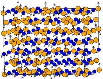
Figure 2. The model of the paramagnetic state considered in this work consists of non-collinear

and fluctuating local moments, which become disordered above the magnetic order-disorder transition temperature, the Cure TC or Neel TN temperature for ferromagnets and

disordered above the magnetic order-disorder transition temperature, the Cure TC or Neel TN temperature for ferromagnets and antiferromagnets, respectively, as illustrated in Fig. 2. Of course, in weak itinerant magnets with qC/qS >> 1like ZrZn2, this picture does not hold. Here the magnetization arises because of specific narrow peaks in the electronic density of states at the Fermi level, fulfilling the Stoner criteria. Under such circumstances, the concept of the moments rotating nearly rigidly probably breaks down and the excitations can be more from electron-hole pairs than from moment rotations [10]. We will not consider weakly itinerant magnets in this review.

At the same time, magnitudes of the local moments do not have to be constant even for

chemically equivalent atoms. They depend on the local chemical environments of the respective atoms, e.g. due to disorder in alloys or the proximity to defects, on thermally induced atomic displacements, as well as on local magnetic environments of the atoms. Moreover, formed by itinerant electrons magnetic moments fluctuate in space and time due to the presence of longitudinal spin fluctuation. These fluctuations are closely linked to the itinerant nature of electron magnetism, where electron-electron exchange interaction is responsible for the formation of local atomic magnetic moments [13]. The longitudinal fluctuations have a significant effect on the high-temperature properties of magnetic materials, influencing the description of their finite-temperature thermodynamics [28]. Longitudinal spin fluctuations can be incorporated into the local moment picture, either self-consistently, at the level of DFT calculations, by replacing the Weiss field in the calculation with a generalized Onsager cavity field in the framework of the disordered local moment picture [29], or at a level of model Hamiltonians [30-34].

An approach described above has been widely used for studies of finite temperature magnetism, but mainly in the context of simulations of magnetic properties, like TC and TN. On the other hand, first-principles simulations of phase stability, thermodynamic and elastic properties of magnetic materials above these temperatures is a relatively young field, despite the fact that Zener underlined the importance of magnetic excitations for the allotropic phase transitions in Fe almost 60 years ago [35]. Körmann et al. have given a comprehensive overview of state-of-the-art computational techniques to thermodynamically model magnetic and chemical order–disorder transitions [28]. Reviewing recent progress in this field with a focus on first-principles

description of paramagnetic materials based on 3d-series transition metals is the main task of this work.

2. Theoretical models for description of paramagnetic state of magnetic materials: general considerations.

To understand the complexity of the problem, let us consider a magnetic material above its Curie or Neel temperature that is in the paramagnetic phase. To describe its thermodynamic properties one must determine the Gibbs free energy:

magn vib el

PM G G G

G = + + , (1)

which contains electronic Gel, vibrational Gvib, and magnetic Gmagn contributions. State-of-the art approach to this type of tasks would be to employ the adiabatic decoupling between the three degrees of freedom, motivating it by the fact that their excitations usually have very different time scales [36]. The separation of the electronic, the fastest, and atomic vibration degrees of freedom are well justified within the Born–Oppenheimer approximation, assuming that lighter electrons adjust adiabatically to the motion of much heavier nuclei, remaining at any time in their instantaneous ground state. Indeed, as discussed in [25] the characteristic time for d-metals as given by intersite hopping is ∼ 10−15 s, while for the lattice vibrations the characteristic time is proportional to the inverse of the Debye frequency, which is of the order of ∼10−12 s. Excitations associated with magnetic degrees of freedom are commonly related to the to the inverse spin-wave frequency, which is ∼ 10−13 s, and therefore they are assumed to be order of magnitude faster than vibrational degrees of freedom, and several orders of magnitude slower than the electronic ones.

On the other hand, in the paramagnetic state the magnetic excitations are qualitatively different from those at the low temperature. In contrast to the spin wave excitations, other transverse as well as longitudinal excitations of the magnetic moments, like the spin flips, dominate. The relevant time scale can therefore be better estimated from the spin decoherence time tdc rather than from the inverse spin-wave frequency. For body-centered cubic (bcc) Fe above TC tdc is of the order of 20–50 fs [11]. Thus, the magnetic degrees of freedom in the paramagnetic state should be considered as much faster in comparison to those in magnetically ordered materials, of the order of 10−14 - 10−15 s. Moreover, it is important to realize that the paramagnetic state is the high-temperature state of a magnetic material. Thus, a consideration of atomic motions is

essential. The time scale given by the Debye frequency is therefore getting less relevant, and one should consider the atomic motions on the time scales familiar from molecular dynamics

simulations. Here the typical time step for a proper description of the (Born–Oppenheimer) dynamics is ~10−15 s. Finally, the potential energy surface can be influenced by magnetic and vibrational excitations. In summary, an argument for the decoupling of electronic, magnetic and vibrational contributions to the free energy, well justified for magnetically ordered materials at low temperatures becomes questionable for the theoretical description of their paramagnetic state.

All the terms in Eq. (1), Gel, Gvib, and Gmagn are coupled to each other and in principle should be treated simultaneously in first-principles calculations of paramagnetic materials.

To complicate the picture further, it is important to underline that the physics of strongly

correlated electron systems recognizes the description of the finite-temperature itinerant electron magnets and the existence of local magnetic moments above TC or TN as one of the central

problems [37]. For a system with itinerant electrons local magnetic moments become temperature dependent. Besides the thermal fluctuations which disorder the moments, a variety of competing many-body effects should be considered, such as Kondo screening and the induction of local magnetic moment by temperature. These effects go beyond the state-of-the-art local (local spin density approximation, LSDA) or semi-local (generalized gradient approximation, GGA) implementations of DFT, and require applications of advanced, but time-consuming techniques, e.g. based on the dynamical mean-field theory (DMFT) [38].

Thus, the problem of the description of the paramagnetic state of magnetic materials appears to be challenging for the first-principles theory. However, the great practical importance of e.g. steels has motivated intense research in the field, and several research groups have dealt with it, from different starting points. In particular, DMFT calculations have been carried out for several systems, despite their complexity. On the other hand, it has been realized that some of the many-body effects can be taken into account, in an approximate way, in the framework of more

traditional density functional techniques. Below we discuss these theoretical developments.

3. Dynamical Mean-Field Theory.

Perhaps the most consistent way to describe the paramagnetic state of a magnetic material with account of correlation effects is given at present by a combination of DFT with model treatments of many-body effects, like the Hubbard model, e.g. within the dynamical mean-field theory. The DMFT [39] maps the Hubbard model, which in principle is a lattice model, onto quantum impurity model subject to a self-consistent condition in such a way that the many-body problem for the crystal splits into a one-body impurity problem for the crystal and a many-body problem for an effective atom. The relevant degrees of freedom at a single site are the quantum states of the atom, while the rest of the crystal is described as a reservoir of non-interacting electrons that can be emitted or absorbed in the atom [40]. The effect of the environment on the site is to allow the atom to make transitions between different configurations. The quantum nature of the

problem requires a hybridization function that plays the role of a mean field and describes the ability of electrons to hop in and out of a given atomic site, ensuring a self-consistency condition to the quantum impurity problem. In the case of weak hybridization the electrons will behave as localized, while in the opposite case they will behave as itinerant. The field is determined consistently: one uses the solution of the quantum many-body impurity problem to build

self-energy for the lattice Green’s function that in turn gives a new approximation for the dynamical mean-field. A combination of DFT and DMFT is realized in the following way: the electronic structure calculation results obtained by DFT methods are used to calculate parameters for a general DMFT Hamiltonian and then the problem defined by this Hamiltonian is solved within the DMFT [41]. More detailed introductory information on the DMFT can be found in [40], fundamental basics of DMFT have been reviewed by Kotliar et al.[38], while a review on recent investigation of real materials with strong electronic correlations by the LDA+DMFT method has been presented by Anisimov and Lukoyanov[41].

Consider the problem of the paramagnetic state of magnetic materials. Solving the quantum impurity problem within DMFT, one describes the spin, orbital, energy, and temperature

dependent interactions of a particular magnetic atom with the rest of the crystal. The uniform spin susceptibility in the paramagnetic state χq=0=dM dHcan be extracted from Quantum

Monte-Carlo (QMC) simulations [37] used for the solution of DMFT quantum impurity problem by measuring the induced magnetic moment in a small external magnetic field. It includes the polarization of the impurity Weiss field by the external field. For a Fermi liquid one expects temperature independent Pauli behavior of χ_q=0. On the other hand, if the local moments survive above the magnetic transition temperature, the uniform spin susceptibility follows the Curie-Weiss law: ) ( 3 2 0 C eff q T T− = = µ χ , (2)

which allows one to extract high-temperature magnetic moments µ_eff and the magnetic transition temperature TC from calculations. Of course, the latter should be overestimated due to the mean-field approximation, underlying the DMFT.

Another important quantity that one can compute using the LDA+DMFT approach for a paramagnetic system is the dynamic local magnetic susceptibility [42]:

ωτ β τ τ µ ω χ z i j z j B loc i =

∫

where µ is the Bohr magneton, _B S is the z-component of single-site spin operator S at site j, and z_j β=T-1_{. Taking analytical continuation of} χ _(iω₎

loc to the real frequency axis ω, one can try to fit loc

χ

Re by the simple Lorentzian form, denoting half-width of the peak at a half-height as δ. δ describes the inverse lifetime of local excitations, and the large is it the smaller is lifetime of the local moments in the paramagnetic state. The static susceptibility in the local-moment regime is given byχ_loc(0) . In contrast to the uniform spin susceptibility, the dynamic local magnetic

susceptibility cannot be measured in experiments, but its temperature dependence characterizes the degree of correlations in the system. χ_loc should be nearly temperature independent in weakly correlated systems, while in strongly correlated systems one expects the Curie-Weiss behavior at high temperatures [37]: ) 3 ( 2 const T loc loc + = µ χ , (4)

For the system with well-defined local moments the DMFT is expected to yield δ ~ T and

loc

µ should be temperature independent, while in the more itinerant system one should see significant temperature dependence of µ_loc.

In original applications of the LDA+DMFT the procedure was carried out without charge consistency. However, state-of-the-art applications of the method include the charge self-consistency, making it possible to calculate the total energy and to access thermodynamic [43] and vibrational [44] properties of paramagnetic materials in addition to the magnetic properties. At the same time, it is important to understand that the DMFT itself contains several

approximations, which should be well understood in its practical applications. Being the mean-field theory, it neglects intersite magnetic exchange, and it should in general overestimate magnetic transition temperature. Magnetic short-range order present in any system not too far above the magnetic transition temperature cannot be captured as well. Note that a comparison of the values of the local and the q= 0 susceptibilities could give a crude measure of the degree of the short range order [37]. Methods to add nonlocal corrections to the DMFT have been

developed, for example the dynamical cluster approximation [45,46], the cellular dynamical mean-field theory [47], and the dual fermion approach [48] . However, their application in simulations relevant for the materials design are still illusive due to very high computational costs.

Another big problem for practical applications of the LDA+DMFT scheme is the existence of two parameters of the model, the Coulomb U and exchange J interaction parameters. Often these parameters are varied to achieve the best agreement between experimental data and calculations for some known and well-characterized property. Within such approach, the model parameters are considered as adjustable parameters. In principle, one can estimate the value for the Coulomb interaction parameter U from the energy separation of the spectral peaks interpreted as Hubbard bands [41]. Moreover, there are computational schemes proposed to calculate U and J from first principles, e.g. employing the constrained random-phase-approximation (cRPA) method [49,50]. However, their use is still quite rare. Unfortunately, the LDA+DMFT calculations are still time consuming, and the method is most often applied to materials with few atoms in the unit cell and with relatively high degree of symmetry. Moreover, until recently forces between atoms were

calculated from the numerical derivation of the total energies, ruling out efficient consideration of lattice dynamics. Fortunately, Leonov et al. [51] has just proposed a novel computational

approach which makes it possible to evaluate interatomic forces within DMFT approach. Still, there is a need for theoretical methods that treat many-electron effects at more approximate level.

4. Spin dynamics

The key point for a theory that aims at simplifying the treatment of the many-body effects in paramagnetic materials is the equivalence between a many-body interacting system with

Coulomb onsite interactions and a one-electron system in fluctuating charge and spin fields. This equivalence is a base of spin-fluctuation theories of itinerant-electron magnetism [26]. In a complete theory, the charge and spin fields are dynamically fluctuating in both space and time. One could try to capture these fluctuations with DFT calculations for a system which magnetic state is excited, and where the arrangement of local moments differs from that in the magnetically ordered ground state and fluctuates with time. Perhaps, ab initio spin dynamics gives the most consistent realization of this approach.

Antropov et al. [9] inspired the interest to this technique, and presented a detailed derivation of the equations about a year later [10]. Starting with basic DFT formalism and considering each electron moving in the average ‘‘charge’’ and ‘‘spin’’ self-consistent fields V (r) and B(r) of the electrons and ions, Antropov et al. derived the equation of motion (EOM) for spin density m(r,t):

) . ˆ ( 2 ) , ( c c i g t t d s × + ∇ ∇ − = m B Ψ*σ Ψ r m , (5)

where g is the gyromagnetic ratio, s Ψ is the electronic spinor, σˆrepresents a vector of Pauli

matrices, and c.c. stays for complex conjugate.

To make the solution of equation (5) possible in practice and to include temperature effects, Antropov et al. introduced the quasiclassical spin approximation [9,10]. They assumed that the magnetization density in the immediate vicinity of an atom has a uniform orientation, divided the space into spheres or polyhedra, and within each such region associated a unit vector ei with the instantaneous magnetization direction. Associating such a region with one particular atom with the local moment Mi=μei, they arrived at the local moment picture, which we discussed in the introduction and illustrated in Fig. 2. The next simplification consisted in introducing the rigid spin approximation (RSA), assuming that the time evolution of the orientation is described by a simultaneous (or rigid) rotation of the magnetization density at each point inside the atomic

sphere or polyhedra. Note that the amplitude of the magnetization density was allowed to change. With these approximations quasi-classical EOM of ab initio spin dynamics take the form:

I e e_{=− ×} µ 2 t d _{, (6)} where e B I=−µ =∂E ∂ (7)

is the first variation of the total energy E for a differential rotation of a local moment, and

therefore in analogy with molecular dynamics can be viewed as a magnetic “force” acting on the spin. It can be calculated, for instance, using the magnetic force theorem within the multiple scattering formalism [52]. To include temperature effects, Eq. (6) can be modified, e.g. in the framework of a stochastic method based on Langevin-type dynamics [10]:

[

]

In Eq. (8) Ri is a relaxation term and fi is a random force at each site i in the system.

Despite the simplifications mentioned above, an approach proposed by Antropov et al. remained computationally demanding. Simulations were performed, but for relatively simple systems, like pure Fe [9,10] or FeNi alloys [6,7]. Further development of the idea was associated with bringing model Hamiltonians into play to calculate the magnetic “force” in Eq. (7). The simplest model can be based on the classical Heisenberg Hamiltonian H_cH:

j i i j i ij cH J ee H

∑

known to work well for transition metals and their alloys [52]. Of course, this means that one goes from quasi-classical to semi-classical description. Indeed, the exchange parameters Jijare

calculated within DFT, thus linking first-principles theory to the classical spin-dynamics. Skubic et al. [12] presented an excellent overview of the semi-classical approach that greatly simplifies the problem. Moreover, they proposed to use more complex Hamiltonian as compared to Eq. (9), adding to the classical Heisenberg Hamiltonian terms corresponding to uniaxial magnetic

anisotropy, dipolar interactions, and the Zeeman term that described the interaction of the magnetic system with an external magnetic field.

One should note however, that while the semi-classical approximation was demonstrated as a useful tool to study spin dynamics in many systems [11,12], very limited number of simulation had a description of the paramagnetic state as the primary task [53]. Several issues have to be considered here, like the importance of longitudinal spin fluctuations, the dependence of

exchange parameters on the global magnetic state of the system, deviations between the classical and quantum solution of the Heisenberg model, and the effect of lattice vibrations.

The lack of longitudinal fluctuations (LFs) was a fundamental drawback of the classical

Langevin-type spin dynamics. Ma and Dudarev [13] proposed a scheme to include LFs in a semi-classical dynamics of evolution of interacting magnetic moments. Their method was based on the generalization of Langevin spin dynamics to a fully three-dimensional stochastic dynamics of moments. In this approach, both the longitudinal and rotational degrees of freedom of atomic spin vectors were treated on equal footing. This removed a fundamental limitation associated with the lack of longitudinal fluctuations in semi-classical spin dynamics equations, but retained the capacity of the method to simulate a very large system of interacting spins.

A key aspect in a development of semi-classical theories that incorporate the longitudinal spin fluctuations has been a generalization of the classical Heisenberg Hamiltonian (9). Several suggestions have been put forward, which could be classified in two groups. The first group was based on an idea of merging the Heisenberg Hamiltonian (9) with a Ginzburg-Landau like energy expansion into a Heisenberg-Landau Hamiltonian [13, 30, 31, 33, 34]:

∑∑

∑

where Ai(n)were the parameters of the Ginzburg-Landau like energy expansion. The second

suggestion by Ruban et al. [32] introduced the longitudinal spin-fluctuation Hamiltonian HLSF

by making the parameters of the classical Heisenberg-type Hamiltonian dependent on the magnitudes of local moments:

j i j i i j i ij i i i LSF J M J M M J M M M MM H ( ) ( , ) ( , , ) , ) 1 ( ) 0 (

∑

∑

∑

In both approaches, the parameters of the Hamiltonians should be fitted to constrained DFT calculations.

Ruban et al. [32] underlined another important aspect of the use of model Hamiltonians, the dependence of the model parameters on the global magnetic state. In particular, they calculated

the parameters of Eq. (11) for the magnetically disordered state simulated with the Disordered Local Moment (DLM) model (see Sec. 5 below). Thus, the parameters of the model Hamiltonian in Eq. (11) have the following physical meaning. J(0)(M) corresponds to the energy of the magnetically disordered state, which represents a system with randomly oriented spins with a fixed value of the magnetic moment M . J(1)(M,M_i)is the energy required to change the value of the spin from the corresponding average value M to the value Mi. The pair exchange

interaction parameter Jij describes the magnetic interaction between atoms in positions i and j in the system where all other local moments were completely disordered. Ruban derived an expression for calculation of Jij in the paramagnetic state [54] using the multiple scattering theory, which differed from that of Ref. [52], where it was derived for a ferromagnetic ground state. As a matter of fact, for many itinerant systems there were significant differences in the results, calculated with the two expressions [54,55]. The problem is well recognized by now, and several groups propose their own schemes for taking into account the dependence of the model Hamiltonians parameters on the global magnetic state for the itinerant systems [56,57,58].

Another interesting question is associated with possible deviations between the classical and quantum solution of the Heisenberg model. This problem has been studied in Ref.[59]. Based on a comparison between numerically exact results obtained from spin QMC simulations and classical simulations for different model systems and various thermodynamic properties,

Körmann et al. have concluded that below TC the classical treatment could deviate significantly compared to the quantum treatment. On the other hand, for high temperatures well above TC as well as for increasing spin quantum numbers quantities such as the internal energy and the specific-heat capacity have approached each other as expected.

5. Models of the paramagnetic state based on static DFT calculations at zero temperature. 5.1 Disordered Local Moment model in the framework of the coherent potential

approximation.

Disordered Local Moment model was introduced by Hubbard [60] and Hasegawa [61]. Gyorffy et al. [25] gave the modern derivation of the DLM and combined it with the LSDA-DFT. Within this model one assumes that the system consisting of all the electrons, although ergodic, does not cover its phase space uniformly in time. Rather, it gets stuck for long times, which we here

denote as the spin-flip time tSF, near points characterised by a finite moment at every site pointing in more or less random directions and then moves rapidly to another similar point. Gyorffy et al. supposed that the motion of temporarily broken ergodicity is mainly characterised by changes in the orientational configuration of the moments. Furthermore, Gyorffy et al. demonstrated [25] that neglecting the spin-orbit interaction and assuming the complete disorder between the local

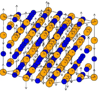
Figure 3. Schematic representation of the Disordered Local Moment model. The paramagnetic state consisting of fully disordered non-collinear and fluctuating magnetic moments (Fig. 2) is approximated by fully disordered, collinear and static picture.

moments the noncollinearity of the local moments (Fig. 2) could be ignored. Note that the model of complete disorder should work well at temperatures T >> Jijmax, where

max

ij

J is the strongest interaction of the classical Heisenberg Hamiltonian (9) for the corresponding system. Thus, within the DLM picture, the local magnetic moments exist in the paramagnetic state above the magnetic transition temperature, but the are fully disordered and collinear (Fig. 3). With this simplification, the magnetically disordered state can be described as a pseudo-alloy of equal amounts of atoms with spin up and spin down orientations of their local moments, and its electronic structure and the total energy can be calculated within the conventional alloy theory using the coherent potential approximation (CPA) [25].

A great advantage of the DLM picture consists of the possibility to formulate a consistent electronic-structure based thermodynamic theory, that accounts for the interplay between the configurational and magnetic degrees of freedom. In particular, Gyorffy and Stocks [62], and then Staunton et al.[63] derived a general formalism to describe the atomic short range order in the compositionally disordered phases, the so-called S(2) method. S(2) is defined as the second derivative with respect to concentration of the grand potential of the disordered alloy, and its physical meaning is related to the effective energy of the interchange of atoms in the alloy, the so-called effective cluster interactions [36]. If calculated in the reciprocal space, S(2) is directly

related to the lattice Fourier transform of the short-range order parameter. In Ref. [54] Ruban et al. combined the corresponding real space appraoch, the generalized perturbation method, with the DLM model. These approaches allowed for the description of the configurational

thermodynmaics in many alloys (for the recent review, see Ref.[36]).

Status of the DLM approach in the many-body lattice models like the Hubbard or s-f exchange “Kondo lattice" model was discussed, e.g. in Ref. [64]. It was argued that though in a complete theory the charge and spin fields were dynamically fluctuating both in space and time, a “static" DLM approximation, where one neglected the dynamics of the fluctuations might capture an important part of the correlations. Indeed, DLM combined with the CPA became equivalent to the “Hubbard III" approximation for the original many-body problem, which jusified the use of the DLM for systems with dominating transverse magnetic fluctuations and explained its success in many applications, ranging from basic simulations of magnetic phase transitions [25] to the design of new steels[65] and hard coatings [66,67]. Moreover, the DLM approach can be combined with techniques, that go beyond the conventional LSDA or GGA implementations of the DFT in terms of the tretment of many-body effects. In particular, it can be easily combined with the so-called LDA+U method [41,68,69], the static mean-field approximation (unrestricted Hartree–Fock) to the many-body problem. LDA+U method was found to be very successful when applied to systems with long-range spin and orbital order, but it was considered unsuitable for the desription of the paramagnetic state of correlated magnetic materials [70,71]. Alling et al. [17,72] demonstrated that a combination of LDA+U with the DLM picture allowed them to lift off this restriction. We should discuss this problem in more details in Sec. 7.4.

On the other hand, DLM-CPA has other limitations, besides the approximate treatment of the many body effects. The codes that implement this approach are most often based on multiple-scattering formalism and involve other approximations, e.g., the spherical approximation for the one-electron potential. This limits a possibility to treating materials with complex underlying crystal lattices and alloys with significant size mismatch between the alloy components, systems with point defects, like vacancies and interstitial impurities, or extended defects, like interfaces, grain boundaries and stacking faults. If local lattice relaxations are large and effects of local chemical environment are important, they cannot be treated explicitly within the single-site approximation, on which the CPA is based. Furthermore, despite the fact that Taylor formulated the CPA for the lattice dynamics problem [73], we are not aware of a broad application of the methodology in practice. Thus, a simultaneous treatment of magnetic excitations and lattice vibrations is hardly feasible at present. Thus, approaches that go beyond the CPA are highly requested.

5.2 Supercell approach

Following [72], let us start with the classical Heisenberg Hamiltonian (9) and introduce the average spin-spin correlation functions for coordination shell α :

∑

where N is the number of atoms in the system. In this formalism, the energy of a magnetic state can be written as:

α α α α Φ n J Emagn =−

∑

where Jα =J0jfor j∈α , n is the number of atoms in the α α -th coordination shell on the lattice.

For example, one can immediately see that the magnetic contribution to the energy of the ferromagnetic state =−

∑

α α

J

EFM , while for the fully disordered paramagnetic state EPM =0,

because in the high-temperature paramagnetic state with the complete disorder between the local moments the average spin-spin correlation functions fulfil the condition

α

α = 0 ∀

Φ , (14).

One way to fulfil Eq. (14) in first-principles simulations is to employ the idea of the so-called special quasirandom structures (SQS) put forward by Zunger et al. to describe chemically disordered alloys [74], and generalized for the case of magnetic disorder by Alling et al. [72]. Because the exchange parameters should decay with distance, one assumes the finite range of the interactions, which simplifies condition (14): Φ_α =0 only for α with J_α ≠0. Indeed, if

0 = α

J , any value of Φ_α does not influence the left-hand side of Eq. (13). Note that while the original condition (14) requires to dealing with in principal infinite system, the SQS condition can be fulfilled in the finite size periodic supercell. Moreover, as has been emphasized in Sec. 5.1, for the ideal paramagnetic state only collinear spin configurations should in principal be sufficient. The formalism is easily generalized to include multi-site interactions [72]. Of course, in using magnetic SQS one should have in mind all the limitations of the conventional SQS methodology for the treatment of configurational disorder, reviewed in details in Ref. [36].

Moreover, as pointed out by Ruban and Razumovskiy [75], if one deals with an ideal Heisenberg model system, the magnetic interactions are constant, and the way condition (14) is satisfied does not matter. Therefore, one can perform averaging over a proper set of magnetic systems. Every member of such a set can have an arbitrary magnetic structure, but their average should fulfil Eq. (14). One method that achieves this goal is the magnetic sampling method (MSM) suggested by

Alling et al. [72]. In the MSM, one generates a set of magnetic distributions with random orientation of local magnetic moments, though without taking care of the obtained correlation functions, in contrast to the SQS approach. This can be easily done, for instance, using a random number generator. Then the electronic structure calculations are carried out for each

configuration, and the average of the obtained total energies is taken as the potential energy of the paramagnetic sample. In Ref. [72] it was shown that for paramagnetic CrN with B1 crystal

structure MSM calculations converged already at 40 different magnetic distributions. Moreover, three different approaches, the DLM-CPA, the magnetic SQS and the MSM gave almost identical results for the potential energy of this system.

It is important to underline that because the goal of the supercell calculations is most often to approximate the potential energy E_PM of the paramagnetic alloy at high temperature T, strictly speaking it should be defined as a thermal average over the ‘fast’ magnetic degrees of freedom [76]: ln σ σ σ PM β = PE (Z) = E

∑

∑

∑

{

}

Z exp is the canonical partition function, P is the thermal σ

probability of a particular (magnetic) configuration σ,

T k = β B 1

, where k is the Boltzmann’s _B constant. E and _σ g are the energy (per atom) and the multiplicity of each magnetic _σ

configuration, respectively. In fact, using Eq. (15) one can check whether the DLM approach is adequate for the problem at hand or not. Indeed, if the condition for the applicability of the DLM

max

ij

J

T >> is fulfilled the potential energy calculated from Eq. (15) should be in good agreement with the result obtained by an arithmetic average over different magnetic configurations. For example, in the case of substitutional (N, V) and interstitial (C, N) impurities in fcc Fe

Ponomareva et al. have found negligible difference between the two averaging methods at the temperatures corresponding to the stability field of austenite [76], which has justified the use of the DLM picture in that study.

Ruban and Razumovskiy [75] also pointed out that one has to be careful using the supercell approach because it provides a DLM-like distribution of the magnetic moments only on average for the whole supercell, while specific local correlation functions are quite arbitrary. In the case of modeling of local defects, such as vacancies, impurities, surfaces, interfaces, one therefore has to perform the corresponding averaging over magnetic configurations locally. Consider, for

(a) (b)

Figure 4. (a) Supercell realization of the disordered local moment model for calculations of the solution energy of an interstial impurity, like C (small yellow atom) in paramagnetic fcc Fe (large red atoms). (b) Using a combination of magnetic special quasirandom structure and magnetic sampling methods, one calculates energies of supercells with different impurity positions in the magnetic SQS representing the host, which are shown here versus the total magnetic moment of Fe atoms located in the first coordination shell of the impurity. Significant variation of the calculated energies depending on the impurity positions in the supercell is clearly seen in the figure.

instance a straightforward use of the magnetic SQS approach for the calculations of impurity solution energies. By placing the impurity at one particular position in the supercell representing the host, the former will sense only one magnetic configuration (Fig. 4a). Indeed, the magnetic SQS approach gives a static picture of the “frozen” magnetic disordered and does not account for the spin dynamics. Note that atomic diffusion processes are several orders of magnitude slower than the magnetic degrees of freedom, therefore on the time scale associated with the diffusion magnetic fluctuations are almost instant. This means that the impurity will sense many different magnetic configurations rather than only one.

Ponomareva et al. [76] has addressed this issue and proposed a combination of the magnetic SQS and MSM approaches for calculations of point defects in paramagnetic hosts. To catch the

dynamic behavior of the magnetic system Ponomareva et al. approximated the paramagnetic material by a set of many magnetic configurations, following the idea of the MSM. However, they combined it with magnetic SQS method, which was used to represent the host and to allow for an accurate description of small energy differences between the systems with and without the impurity. The proposed MSM-SQS scheme for calculation of solution enthalpies is as follow. First, one uses the magnetic SQS method to simulate the paramagnetic host. Next one varies

magnetic distributions around the impurity by changing its positions inside the magnetic SQS and calculates the total energies, which depend strongly on the impurity position (Fig. 4b). Then one averages the energies using Eq. (15) and obtains the potential energy of the paramagnetic system with the defect. If the convergence with respect to the SQS size is achieved, the magnetic SQS for the host with or without the defect ensures that Eq. (14) is fulfilled globally, while MSM sampling of the position of the defect inside the SQS ensures the fulfillment of Eq. (14) for the average local spin-spin correlation functions on the defect site.

In using the supercell realizations of the DLM picture, one should keep in mind that the random distribution of spins on the underlying lattice does not guarantee that the result of the self-consistent calculations corresponds to the ideal DLM state [75]. In the DLM it is assumed that all the local magnetic moments for chemically equivalent atoms have exactly the same

magnitude. This is usually not the case for the systems with the itinerant type of magnetism treated within the supercell approach. Another important issue is related to calculations of interatomic forces and a possibility to account for the local lattice distortions, e.g. around the defects. In fact, this is one of the main motivations for the use of the supercell approach rather than the DLM-CPA scheme.

Unfortunately, fixing a magnetic state in time would lead to artificial static displacements of atoms off their lattice sites due to forces between the atoms with different orientations of their local moments and with different local magnetic environments. In the case of CrN this was clearly demonstrated in Ref. [27]. On the other hand, in a real paramagnet the fluctuations of the local moments in time should average out and suppress this effect, at least partially. The

existence of the local lattice relaxations for the ideal crystal with chemically equivalent atoms at high symmetry positions is an obvious artifact of the model that describes high-temperature state with fluctuating spin fields and moving atoms in a static picture suitable for conventional

electronic structure calculations at T=0K. It can have significant effect on the calculated potential energy. Figure 5 illustrates this for the case of CrN. The static relaxation energy of the fixed magnetic SQS (circles) is quite large - 0.036 eV/f.u., and unphysical. This is a clear signature of the brake-down of an attempt to model a space and time fluctuations with a purely spatial disorder. However, the artificial effects of the local lattice relaxations can cancel each other in calculations where potential energies of two paramagnetic systems have to be compared, for instance in calculations of the impurity solution energies or mixing enthalpies of the

Figure 5. (Color online) Relaxation energies (in eV per f.u.) in the 64-atom CrN supercell as a function of relaxation iteration step. The spurious and relatively large static relaxation energies of the fixed magnetic SQS configuration (black circles) is contrasted with the relaxation energy of the magnetic sampling method (green diamonds) which is nearly vanishing within the accuracy of the method. Here a series of magnetic samples is considered and the forces acting on each nucleus in all the samples are averaged. This average force is then used to guide the nuclei to their optimal static positions. Also the energy of the SQS configuration calculated on the structure obtained with the magnetic sampling method is shown for comparison (red squares). Here we perform one small relaxation step in all the calculations of the magnetic samples. Then we put together the new positions and average them, resulting in the actual relevant new

positions. The agreement between the two later methods with magnetic SQS calculations without local lattice relaxations underlines artificial nature of the conventional static approach. Details of calculations are the same as in Ref. [72].

5.3 Spin wave method

Besides the above-mentioned complications of the supercell approach, it becomes quite time consuming in the case of random alloys or large and inhomogeneous systems. Ruban and Razumovskiy have proposed another scheme that fulfills condition (14), the spin wave method (SWM) [75]. They considered a set of the planar spin spirals with the azimuth angle π/2 for all the wave vectors q in the corresponding Brillouin zone and showed that the spin-spin correlation function for a superposition of all the spin spirals with different wave vectors averages to zero, thus fulfilling Eq. (14). The energy of the paramagnetic state in the SWM is given by the integral over the Brillouin zone of the energies of each planar spin spiral with the wave vector q. In practice, one does this using the special point technique, requiring to carry out DFT calculations for a finite set of q-vectors.

In application of the SWM method for calculating properties of Fe and Co, the results were found to be very close to those obtained by means of the DLM-CPA calculations. However, the former can be combined with the supercell geometry, for example to describe defects or local relaxations in chemically disordered systems. In particular, the SWM allows one to calculate the defect-formation energies, elastic constants [75], and phonon spectra [78]. One of the advantages of the spin-wave method is a possibility to model a magnetic state with specific magnetic short-range order, the effect, which is difficult or impossible to study with other approaches described above. Of course, the method describes the high-temperature paramagnetic state as a set of

non-interacting magnons. This can be questioned from the fundamental point of view. On the other hand, semi-classical spin-dynamics simulations using Eq. (6,7,9) carried out to elucidate a long-standing controversy regarding the existence, or otherwise, of spin waves in paramagnetic bcc iron, point to their existence [53]. In addition, one has to remember that the justification of the SWM involves the independence of the exchange parameters on the magnetic state, which is not the case in many itinerant systems. One should bear in mind, however that the SWM method gives the field very new and interesting idea. Its evaluation in future applications will contribute to better understanding of its advantages and limitations.

6. Lattice dynamics of paramagnetic materials.

In most applications, the simulations of the magnetic materials in the paramagnetic state are still carried out at the fixed crystal lattice, neglecting contributions from lattice vibrations, which ought to be increasingly important when one goes from low-temperature magnetically ordered state to the high-temperature paramagnetic state. As has been pointed out in Sec. 3, the

LDA+DMFT calculations are too time consuming. Moreover, at present forces within the

LDA+DMFT approach have only been calculated directly from the derivative of the total energy. In particular, this approach was employed by Leonov et al. [44] in the calculations of the phonon dispersion relations for Fe. Leonov et al. computed the lattice dynamics of paramagnetic iron using the GGA + DMFT approach in combination with the method of frozen phonons. The phonon frequencies were calculated by introducing a small set of displacements in the

corresponding supercells of the equilibrium lattice, which results in a total energy difference with respect to the undistorted structure. Unfortunately, computational costs associated with these types of calculations are very high at present. This makes it difficult to efficiently couple magnetic and vibrational degrees of freedom within the DMFT calculations in a simultaneous treatment of molecular and spin dynamics, needed for a description of materials behavior at high temperature and fro calculations of all free energy contributions to Eq. (1) at the same footing, as discussed in Sec. 2.

Figure 6. (Color online) Schematic illustration of DLM-MD algorithm. See text for more discussion.

Theoretical formalism that combines quasi-classical spin dynamics with molecular dynamics was presented in Ref. [10]. However, it is too time consuming and to the best of our knowledge, it is not realized in practice yet. A combination of semi-classical spin dynamics and molecular dynamics should be more numerically efficient, and there is a significant progress in this direction [79,80]. For example, Perera et al. [81] have simulated properties of bcc Fe at room temperature, while Tao et al. [53] have studied its spin dynamics above TC. However, in addition to the problems of the semi-classical approach discussed in Sec. 3, one would have to treat a dependence of effective exchange parameters on the distances between atoms. The latter may be significant [58,82]. Thus, more approximate solutions to the problem are sought.

6.1 Disordered local moment molecular dynamics.

Steneteg et al. [27]suggested to implementing the DLM picture in the framework of ab initio molecular dynamics (MD) within the DLM-MD method. DLM-MD algorithm shown in Fig. 6 realizes numerically the concept of of temporarily broken ergodicity [25] discussed in Sec. 5.1.

According to it the magnetic subsistem gets stuck for time tSF at a point of the phase space corresponding to the particular magnetic configuration and then moves rapidly to another point. Remember that tSF denotes the time between spin-flips which is long enough (in the particular case of Fig. 6 it corresponds to 10 fs). Steneteg et al. made an approximation that the magnetic state of the system is completely randomly rearranged with a time step tSF, and with a constraint that the net magnetization of the system should be zero. To simulate a paramagnetic system, they initialize calculations by setting up a supercell where collinear local moments are randomly oriented and the total moment of the supercell is zero. Then they run collinear spin-polarized MD for the number of MD time steps. Denoting the MD time step as tMD and requiring that tMD << tSF, the number of the MD time steps that the system stays in the same magnetic state is given by

MD SF SF

MD t t

vary as dictated by the self-consistent solution of the electronic structure problem at each step of the MD simulation. In principle, the orientations of the magnetic moments are not restricted, so they are allowed to flip as well. Thus, the net magnetic moment in the simulation cell should be checked to make sure that the system remains in the DLM state. When NMDSF steps of the MD are

executed the spin state is randomized again by setting up another configuration of disordered local moments, while the lattice positions and velocities are unchanged, and the simulation run continues (Fig. 6). In several applications of the DLM-MD [27, 77] it was demonstrated that the algorithm depicted in Fig. 6 was numerically stable and led to well-converged values of

observable properties, like the potential energy.

Of course, tSF remains the model parameter, which cannot be determined self-consistently within DLM-MD simulations. In fact, spin-lattice dynamics simulations for ferromagnetic bcc Fe at 300 K [79] demonstrated that the characteristic time scale for the quasiperiodic motion of an atom is of the order of 0.1 ps (which is the inverse Debye frequency of the material). The time scale that characterizes the dynamics of precession of atomic spins is significantly shorter, of the order of fs. Thus, following arguments given in Sec. 2, tSF value of the order of 10 fs should be

reasonable, though it might be system-dependent.

As a matter of fact, Steneteg et al. conducted an additional numerical experiment that allowed them to argue for their choice of tSF (in Ref. [27] DLM-MD calculations were carried out for paramagnetic cubic B1 phase of CrN). They analyzed the Cr- Cr metal nearest neighbor distances, and separated them into pairs with parallel and antiparallel orientations of the local moments. Thus, the effect of tSF on the distribution of pair distances became apparent. If tSF was very short, ~10 fs, there were no noticeable difference between the two sets of pairs, indicating that the atoms did not have time to adjust their positions for the current orientation of local magnetic moments. If tSF was increased to 100 fs, the atoms had sufficient time to move towards the energetically more favorable positions, leading to an observable shift in distances between pairs with parallel and antiparallel local moments. We could not rule out a possibility of

statistical correlations between the atomic distances and the orientation of atomic moments in a dynamically changing paramagnetic phase. However, to the best of our knowledge it has never been reported in experiments. Moreover, its appearance would be contra-intuitive. Therefore, Steneteg et al. argued [27] that in practical applications of the DLM-MD one should use smaller values of tSF, that would ensure the absence of differences in distances between atoms with parallel and antiparallel local moments. Importantly, they also observed that the potential energy shift obtained in the DLM-MD simulations for paramagnetic cubic CrN was ~1 meV/f.u. for tSF less than 15 fs, while it increased substantially for the larger values tSF . The presence of an energy plateau on the potential energy vs tSF curve may justify further the choice of short spin-flip times in DLM-MD simulations. In fact, it indicated that one could use the adiabatic approximation and to consider spin-flips as fast degrees of freedom with respect to atomic motion. The adiabatic approximation could significantly simplify the simulations of lattice dynamics in paramagnetic materials, as will be discussed in Sec. 6.2.

Shulumba et al. [83] used the DLM-MD approach to develop a framework for calculation of the Gibbs free energy of a paramagnetic material, Eq. (1), which coupled all the terms, Gel, Gvib, and Gmagn to each other and treated them simultaneously in first-principles calculations. Shulumba et al. has combined the DLM-MD simulations of disordered magnetism with the temperature-dependent effective potential method [84] to obtain the vibrational contribution to the free energy. This has made it possible to model the phase stability of a magnetic material in its high-temperature paramagnetic phase, including high-temperature-induced anharmonic and harmonic vibrational, as well as the magnetic effects simultaneously. Shulumba et al. have applied the technique to investigate the phase diagram of CrN and have found that the vibrational contribution have favored the stability of the cubic paramagnetic phase with respect to the orthorhombic antiferromagnetic phase. The predicted temperature for the transition has been lowered as compared to the static calculations, bringing it in better agreement with experiments. Once again, here we deal with a new methodology, and its evaluation should take some time. Major approximations in the present realization of the DLM-MD method, which are likely to introduce inaccuracies, include the usage of collinear moments, the temporarily broken ergodicity of the DLM approach, and the existence of the parameter tSF. In addition, so far the scheme has

been applied in simulations of very good Heisenberg systems.

However, our recent results indicate that also more itinerant systems, like fcc-Fe can be

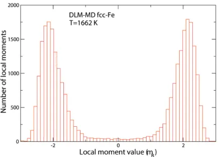
addressed with DLM-MD. Figure 7 shows a histogram of resulting values of local Fe magnetic moments during several pico-seconds run of DLM-MD simulations of fcc-Fe at 1662 K, a temperature just below the gamma-to-delta transition. The figure shows that the vast majority of Fe local moments have magnitudes around 2 μB, but they point into positive or negative

directions depending on their initial orientation. Nevertheless, these results illustrate that there is a considerable variation in magnitudes of the moments. This variation is not related to the

longitudinal spin fluctuations discussed in Secs. 2 and 4, but is instead the direct impact of atomic vibrations, as well as sensitivity of magnetic interactions to the local magnetic environments. Thus, the result shown in Fig. 7 explicitly demonstrates that lattice vibrations and local

environment effects have to be considered in a quantitative description of the paramagnetic state of itinerant magnets. Clearly, the DLM-MD technique has high potential to become a valuable tool for studies of magnetic materials at high temperature.

Figure 7. Histogram of resulting values of local magnetic moments during several pico-seconds run of DLM-MD simulations of fcc-Fe at 1662 K.

Figure 8. (Color online) The Hellmann-Feynman forces in xˆ, yˆ, and zˆ direction acting on a Cr atom (open symbols) and a N-atom (solid symbols) for each MSM configuration of the supercell. The lines indicate the accumulated average of the forces over MSM configurations in each direction for the Cr-atom (solid lines) and N-atom (dashed line). Details of calculations are the same as in Ref.[72].

6.2. Averaging of interatomic forces in the adiabatic limit.

In the adiabatic limit, qualitatively justified in Sec. 6.1, the magnetic degree of freedom is fast with respect to lattice vibrations. This means that the instantaneous forces acting on the atomic nuclei will change rapidly in the paramagnetic state of the system, on the same time-scale as the fluctuations of the local orientations of the magnetic moments. Thus, the relevant forces that determine lattice dynamics are not the instantaneous forces of any particular magnetic configuration. Instead, a better approximation for the lattice dynamics should use the forces averaged over the magnetic fluctuations to govern the nuclei in its motion. In particular, in the adiabatic approximation for the paramagnetic state the fluctuations of the magnetic

configurations are much faster than the relaxation of the nuclei to their equilibrium positions. Thus, the forces acting on each nucleus (the forces averaged over the magnetic fluctuations on the time scale relevant for the lattice dynamics) can be approximated with the forces averaged over different magnetic configurations.

To illustrate this concept we consider the case of paramagnetic B1 CrN without defects. In this system, due to symmetry, there should not be any static lattice displacements of the atoms away from the ideal lattice points. This means that the forces averaged over the magnetic fluctuations on the time scale relevant for the lattice dynamics should be zero. Figure 8 shows calculated Hellmann-Feynman forces acting on a Cr and a N atoms placed on ideal B1 lattice positions in the supercells with different magnetic configurations, generated in the framework of MSM simulations (Sec. 5.2).

Typically, the forces are rather large reflecting the magnetic strain effects in CrN discussed in Ref. [85] and the low symmetry of each structure induced by the magnetic disorder. However, considering the average force of a series of MSM samples, the situation is very different. In fact, the average forces are converging towards zero already after 40 iterations, which coincides with the convergence of the potential energy for this system [72]. This means that the cubic symmetry of B1 CrN is retained only in calculations that use the average forces.

Thus, the following strategy for calculating forces acting on individual atoms in the paramagnetic state of magnetic materials can be used in the adiabatic limit. A series of magnetic configurations are considered and the forces acting on each nucleus in all the samples are averaged. Then this average force is used to determine the dynamics of nuclei in MD or phonon calculations. In fact, Ruban and Razumovskiy [75] have used this strategy in calculations of phonon dispersion

relations in paramagnetic bcc Fe by means of the SWM. Körmann et al. [86,87] employed it in the spin-space averaging method (SSA) coupled to the magnetic SQS method for simulations of lattice dynamics in bcc and fcc Fe by using. A justification of the adiabatic approximation presented here provides a support to these works.