A TIME DEPENDENT FLOW MODEL FOR THE INNER REGION
OF A TURBULENT BOUNDARY LAYER
by
Ho-Chen Chien and V. A. Sandborn
Department of Civil Engineering
Colorado State University
April 1981
This research was carried out under the Naval Sea Systems Corrnnand
General Hydromechanics Research Program Subproject SR 023 01 01,
aJministered
bythe David W. Taylor Naval Ship Research and
Develop-ment Center, Contract N00014-80-C-0183.
A TIME DEPENDENT FLOW MODEL FOR THE INNER REGION OF A TURBULENT BOUNDARY LAYER
Response of ' the flow variables to external driving forces is
non-linear for shear flows. For the turbulent boundary layer case, surface shear stress fluctuations of magnitude as great as the mean
value are observed. For flow near the surface Prandtl' s turbulent boundary layer approach of employing averaged Reynolds equation and a
turbulence closure model is insufficient to account for surf ace shear fluctuations. A model which incorporates a discrete time dependent solution for the inner region of the turbulent boundary layer is pro-posed. The model requires stochastic averaging of the time dependent solution to account for the random aspect of the flow.
The physical model for the flow near the surface is based on the bursting cycle observed in the inner region of a turbulent boundary layer. Localized pressu:te gradients created in the valleys of the
large scale structures of the outer region of the flow are assumed to
be the origin of the bursting process. This model treats the sweep motion as an impulsively started flow over a flat plate. An averaging technique is demonstrated to predict the important features of the surface shear stress.
In order to confirm the time dependent model assumptions, measurements of the probability distribution and cross-correlation of
the longitudinal turbulent velocity and the surface shear stress were evaluated. The sweep-scale, sweep-direction1 and origin of the
probability density distributions of the velocity near the surface and the surface shear stress are found to be similar. However, the velo-city probability distribution changes rapidly with increasing distance from the surface.
As implied by the time dependent model for the surface shear stress, the magnitude of the large surface shear stress would be sub~
stantially changed if the sweep motion could be modified. A series of
thin, metal plates were employed to block thE! instability from reaching the surface. Results show that the mean value of surface shear and the large magnitude fluctuations of surface shear stress were reduced significantly. The variation in surface shear was found to be extremely sensitive to slight angle of attacks of the plates.
Ho-Chen Chien
Civil Engineering Department Colorado State University Fort Collins, Colorado 80523 Spring, 1981
I II III
IV
v
VI
viii ixLIST OF TABLES .
LI ST OF FIGURES
LIST
OF SYMBOLS . xiiiINTRODUCTION . . .
REVIEW OF THE TURBULENT BOUNDARY LAYER STRUCTURE . .
2.1 Early Model . . . . 2.2 Detailed Evaluation of the
Turbulent Boundary
Layer
Structure . . . .SHEAR STRESS
FLUCTUATIONS . . . . .
3.1 Physical Model . . . . 3.2 Simplified Time Dependent Model .. 3.3 Stochastic Averaging TechniquesEXPERIMENTAL SETUP AND PROCEDURE
4.1 Wind Tunnel . . . .
4.2 Instrumentation . . . . ... .
Hot wire probes . . . .
Correlation and probability analyzer Tape transport . . . . .
Time percentage Analyzer Small size pitot tube . . Height indicating system
4.3 Evaluation of the Hot-wire Signals
EXPERIMENTAL RESULT
AND
DISCUSSION . . .
5.1 The Flow Field Over the Test Model
5.2 The Probability Distributions of Hot-wire and Surface-wire Signals . . . . 5. 3 C,onvecti ve Velocity Measurements . . . .
5.4 Cross-correlation Between Surface Shear Stress
and Streamwise Turbulent Velocity .
5.5 Surface Shear Stress Modification . . . .
CONCLUSIONS
REFERENCES .
APPENDICES
A -
DERIVATION OFEQUATIONS (19), (20) AND (21)
B -
DERIVATION
OFEQUATION (32) . . . .
C - FLOW CHART FOR THE COMPUTATION OF P(tw) DUE TO AN
ASSUMED VELOCITY DISTRIBUTION P(U ) .
D -
EVALUATION OF THE MAXIMUS SPACE-TIME
cCORRELATIONS . . . .
vi 1 3 3 4 15 15 20 28 35 35 36 36 37 38 38 38 39 39 40 40 42 4444
4952
55 61 63 65 66ChaJ;>ter TABLES ••
FIGURES
• , ..!. • vii Page Bl 94cf
f f f ' 0 FO' Fl F(f) g Gl' G2 H h L 1 N. l. N 0 P( ) Ap R eRa
R t u w Dimension Skin friction coefficientTransformed velocity defined in Equation (11)
Frequency 1/T
=
a£/o~ ~=O defined in Equation (32)Series solution assumed for f, Equation (17)
One-dimensional frequency spectrum function T Transformed velocity defined in Equation (11)
Series solution assumed for g, Equation (18)
Form factor
High-pass filtered frequency signal Characteristic length in x direction Low-pass filtered frequency signal
Number of At* intervals corresponding to f'
within ith
£'
window 00
Total number of At* invervals used Probability density function
L
Pressure difference M/LT2
Reynolds number based on U and c L
Reynolds number based on momentum thickness Cross-correlation coefficient between surface shear stress and velocity u
(R )
t u max Maximum R t u value for a cross-correlation curvew w
T Mean bursting period T
T T s
t
Non-dimensional mean bursting period, TU~/5
Total summation time used for correlation measurements Time xiii T T T
Symbol
At
.6t maxu, v
u
c u,v 0 0 u ,v .6W x x y z Definition Transformed time=
l/~ Non-dimensionalized timeTime increment used in correlation measurements Maximum time delay when (R ) i~1 obtained
t w u max
Mean velocity components in the x and y directions
Characteristic velocity
Most probable characteristic velocity Convective velocity
Shear velocity Freestream velocity
Instantaneous velocity component in x, y
direction
Velocity fluctuations in x, y direction
Non-dimensionalized velocity in x, y direction Time mean value of product u1 and v'
Longitudinal separation between the lead wire and the rear wire of a dual hot wire probe Averaged x-coordinate of the location of instability origin measured upstream from the surf ace sensor
Streamwise coordinate along the surface of the test model
Coordinate normal to the surface of the test model
Lateral coordinate normal to x and y measured from center of tunnel
x0,y0,z0 Non-dimensionalized coordinate in x, y and z direction
x*
Non-dimensional x coordinate,=
xUt/v xiv Dimension T T L/T L/T L/T L/T L/T L/TL/T
L/T L/T L2/T2 L L L L LSymbol y-1~ y 6
e
v
p t w t w w Definition DimensionNon-dimensional y coordinate,
=
yU/v Non-dimensional z coordinate,=
zUt/v IntermittencyBoundary layer thickness
Displacement thickness of boundary layer Transformed independent variable define in Equation (10)
Momentum thickness of boundary layer Kinematic viscosity
Transformed independent variable defined in Equation (16)
Mass density
Surface shear stress Mean surf ace shear stress
Most probable surface shear stress measured Transformed independent variable defined in Equation (10)
An empirical constant defined in Equation (36)
xv L L
M/L3
M/LT2
M/LT2M/LT2
INTRODUCTION
Since Prandtl introduced the concept of a boundary layer in 1904, the viscous effects on the flow adjacent to a solid bound~ry have
re-ceived a great deal of attention. The laminar boundary layer problem has been solved numerically for a wide range of flow condition. How-ever, the turbulent boundary layer problem is still far from being solved due to its complex nature. Attempts which paralleled the tech-niques employed in solving the laminar boundary layer problem were also applied to the turbulent cases. The eddy viscosity (or mixing length) concept still is viewed as an engineering technique to evaluate turbu-lent shear flows. Conventionally, a model which divided the turbuturbu-lent boundary layer into an inner region and an outer region was
hypothe-sized. Considerable amount of effort has been made to obtain better estimates of the mixing length and eddy viscosity for the two distinct regions of a turbulent boundary layer . The introduction of the idea of eddy viscosity substitutes long- time averaged statistical quantities for the time dependent properties which are inherent to turbulent flow. While of val~e in limited engineering applications, the early models have for the most part required a great deal of empirical input.
In the last two decades, as a result of the improvement of experimental techniques and the advance of electronic computer tech-nology, a great deal of information about the turbulent boundary layer has been obtained. The new information has led to a better understand-ing about the structure of the turbulent boundary layer. Detailed in-vestigation of flow properties in the near wall region, and the outer
two· regions. A large scale motion prevails in the outer region, while the bursting phenomenon is the most important feature in the near wall region. However, the relationship between the large scale motion and the bursting phenomenon is not well understood. It is also necessary to relate the features to the important properties, such as surface shear stress.
In the present study, a physical model which describes a possible connection between the large scale motion and the bursting phenomenon is hypothesized. Following this complex model, a simplified time de-pendent model for the surface shear stress under a turbulent boundary layer was employed to illustrate the importance of time.dependent solu-tion of a turbulent flow. A stochastic averaging technique was devel-oped to account for the random aspect of flow in predicting the surface shear stress. Predicted surface shear was compared with experimental results by assuming a Gaussian or a modified Rayleigh probability dis-tribution of the sweep motion. Experimental evidence was obtained to support the time dependent model. Experiments were performed over a nearly zero pressure gradient surface in a small wind tunnel. Time dependent data evaluated include; convective velocity, probability and correlation of the turbulent velocity and surface shear stress. A simple, thin plate devices was used to modify the structure of the flow near the surface, which in turn reduced the surface shear stress. The device was based on the implication of the model for the flow in the .inner region and its relation to the surface shear stress. The results
REVIEW OF THE TURBULENT BOUNDARY LAYER STRUCTURE 2.1 Early Model
Since Prandtl introduced the concept of a boundary layer in 1904, the viscous effects on the flow adj a cent to a solid boundary have re-ceived a great deal of attention. A boundary layer could be either laminar or turbulent. The laminar boundary layer problem can be solved numerically, however, the turbulent boundary layer problem is still far from being solved due to its complex nature. Pioneer studies made by Prandtl, von Karman and others contributed considerably to the early understanding of turbulent boundary layer characteristics. Convention-ally, two distinct regions in a turbulent boundary layer were hypoth-sized. In the "wall", or "inner" region, the viscous effects are important; while in the "outer" region, the turbulent transport of momentum is dominant.
Attempts which apply the same technique employed in solving the laminar boundary layer problem were also used to evaluate the turbulent cases. One of the earliest approaches was the concept of eddy visco-sity introduced by Boussinesq. Prandtl constructed the mixing length hypothesis to relate the turbulent shear term to the mean veocity gradient. Followed the two-region model of the turbulent boundary
layer, numerical evaluation of the mixing length assumed that it in-creased nearly linear with distance from the wall in the wall region, and that it remained nearly constant over the outer region.
Over the ensuing years, certain refinements of the model were made, mainly regarding the evaluation of the mixing length hypothesis. Van Driest (1956) forsaw the fluctuating nature of the fluid near the
wall and suggested a damping factor for the eddy viscosity in this area. Townsend (1956) suggested the use of a mixing length which was corrected in accordance with the intermittency factor in the outer region. Other refinements, such as considering the entrainment proper-ties of turbulent boundary layer, Head (19.58), have led to some im-provements in predicting the boundary layer properties.
Parallel to the above model, Clauser (1956) suggested that the outer region of the turbulent boundary layer could be treated as a laminar boundary layer having a thin sublayer of a different fluid with much lower viscosity next to the wall. Measurements of flow variables in the sublayer region, which reflected the randomaspect of turbulent shear flow, made before 1957 was summarized by Corrsin (1957). These measurements revealed the existence of large magnitude fluctuations of surface shear stress, surface static pressure and boundary layer thickness.
2. 2 Detailed Evaluation of the Turbulent Boundary Layer Structure In the last decade more detailed information about the turbulent boundary layer structure has been obtained. This new information has
led to a better understanding of the structure of turbulent boundary layers; however, a consistent, workable model for the flow has proven elusive. Recently developed, special, photographic techniques have made visualization of the developing turbulent boundary layer possible. Figure 1 is a sketch of observations and Figure 2 shows a photograph of a turbulent boundary layer developing along flat plates with zero pres-sure reported by Falco (1977) and Nagib et al. (1979), respeetively.
Different aspects of the flow can be seen in the two figures. Figure 1 shows the overall view of the general shape of the large scale
Figure 1. Sketch of turbulent boundary layer obtained by smoke visualization by Falco (1977) at R8 : 4000.
Flow
---...
I
Region where downward sweep motion
Iis seen near the boundary
Figure 2. Photograph of smoke in a turbulent boundary layer reported by Nagib et al. (1979).
motion and the typical smaller eddies rolling over it. Figure 2 illustrates the interface between the large scale turbulent motion and the turbulent outer flow. The streamlines of irrotational, non-turbulent flow in the valley between two consecutive large scale turbulent bulges is shown in Figure 2.
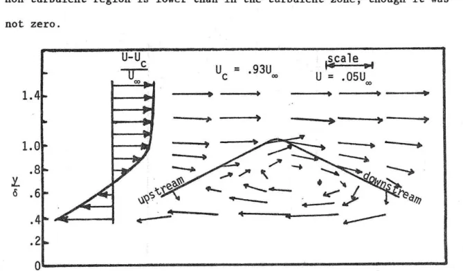
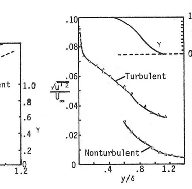
A qualitative picture of the velocity distribution in a large scale bulge and its surrounding fluid was obtained by Blackwelder and Kovasznay (1972), using conditional sampling techniques to evaluate the hot wire signals. Figure 3 shows their results, wherein U c = 0.93 U 00 represents the mean velocity of the turbulent bulge. The rotational nature of the large scale motion in the bulge was demonstrated by Blackwelder and Kovasznay (1972). The local velocities at the front and back of the interfaces, measured by Kaplan and Laufer (1969) using a ten-hot-wire rake across the boundary layer, are shown in Figure 4. It was found that the downstream side of the interface moves faster than the upstream side. Kovasznay et al. (1970) reported zone averages of the fluctuating and streamwise mean velocity components, as shown in Figures 5 and 6. Within the non-turbulent zone the fluid moves faster th{ln it does in the turbulent zone. The turbulent intensity in the non-turbulent region is lower than in the turbulent zone, though it was not zero.
y_
1.41.0
.8
0.6
.4
.2
U-U
c
-u-
00 ~ ).,
...__
....
_
.....
...,..1
~cale,.,
U
=
.05U
00 Ji. ~""'
di•
-:.-
:;.
>
'!J..---..
,,
...
~ "'eiil!JO'---·---Figure 3. Velocity distribution in the outer region of the boundary layer obtain~d by Blackwelder and Kovasznay (1972).
1.
u
u
00.8
y/o
o Downstream •Upstream 1 1.2Figure 4. Velocity distribution at the turbulent bulge interfaces obtained by Kaplan and Laufer (1969) .
1.Q---~_,
Nonturbulent
~-,,,,,,."
' o/c-_,,,.,r/o""
u
u
.95
00.9
.,7
/<?
-- /
/..<...Turbulent
//<,
\Y
.6
.8
y/o
'
'
',
... ...1.0
Figure 5. Zone averages of the streamwise velocity component reported by Kovasznay et al.
(1970). 1.0
,a
.6
.4
.2
0 1.2 y.
10---~---1
y.08\
'-f't
.06
'-~TurbulentIUT'
"+-~
04
~
0.02
\ .
Nonturbulen>"'--·
0
----~---~----=-~-. 4
.8
1.2
y/o
Figure 6. Zone averages of the intensity of the streamwise ve-locity fluctuations reported by Kovasznay et al. (1970).
From the illustrations of Figures 3, 4 and 5, it appears that in the valleys of the consecutive large eddy structures there is a
loc.alized pressure gradient~ which tends to push the fluid inward
toward the wall, and alSo accelerates the fluid on the upstream side of the turbulent bulge. The local streamline curvature near the wall, which would imply a local p·ressure variati'on :ls indicated in Figure 2. The non-turbulent fluid is seen to be thrust almost to the surface. Although the photographs made by Falco (1977) and Nagib et al. (1979) show the large scale coherent structure in the outer region of the turbulent boundary layer, the structure buried in ·the confined wall region is not discernible. Special equipment and techniques are being used to explore the turbulent structure in· the wall region. Kline et al. (1967) conducted visual studies by using a hydrogen bubble tech-nique. Corino and Brodkey (1969) observed motions of suspended colloi-dal particles in the wall region of a circular pipe flow by using a high-speed camera moving with the flow. Combined visualization and hot-wire anemometer techniques were also employed by researchers such as Kim et al. (1971), F~lco (1977, 1980) and others.
Visual studies 6f Kline et al. (1967), Corino and Brodkey (1969) and K:lm et al. (1971) revealed the existence of a somewhat well-organized but spatially and temporally dependent motions within the wall region. A large scale, streaky structure and an intermittently
occurring~ violent bursting process were observed in the wall region.
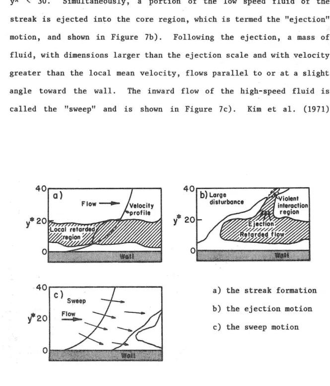
A cycle of the bursting phenomenon was described with the help of sketches, Figure 7, by Corino and Brodkey (1969). Each sketch of Figure 7 shows an important step in the motion involved in a bursting cycle.
First, near the wall low-speed streaks form and gradually grow to a vertical dimension of yl( :: 10, as shown in Figure 7a). When the
streak reaches y"~ ::: 10 it starts to oscillate and continues · to grow.
The oscillation amplifies, as it continue to rise, until it becomes unstable and suddenly breaks into turbulent motion at a height of 10
<
y'i~
<
30. Simultaneously, a portion of the low speed fluid of thestreak is ejected into the core region, which is termed the "ejection" motion, and shown in Figure 7b). Following the ejection, a mass of fluid, with dimensions larger than the ejection scale and with velocity greater than the local mean velocity, flows parallel to or at a slight angle toward the wall. The inward flow of the high-speed fluid is called the "sweep" and is shown in Figure 7c). Kim et al. (1971)
40
a) 0 40--~~~~~~_,.,...,,,,_--s b) Large disturbancey*
20 0Figure 7. Steps in the flow cycle near the wall. Reported by Corino and Brodkey (1969).
provided photographs of streak-lines using hydrogen bubbles for each stage of the bursting phenomenon. Readers are referred to Kim's report for more details.
Associated with the sequence of motions in bursting, occasionally part of the low speed ejected fluid is deflected back toward the wall and at the sam~ time incoming, accelerated fluid is reflected outward
away from the wall. These motions are called "inward interaction" and "outward interaction" respectively. Combinations of streamwise and vertical velocity fluctuations, u' and v', as shown in Table 1 are used to designate these motions.
Table 1. Signs of u', ·v' and u'v' related to motions in a bursting cycle ..
Type of Motion Sign of u' Sign of v' Sign of u'v'
Ejection +
Sweep +
Inward Interaction +
Outward Interaction + + +
Flow properties of each motion, especially the Reynolds shear stress - p u'v', measured in the near wall region by Willmarth and Lu (1971), and Brodkey et al. (1974), indicate the importance of bursting in the generation of turbulent energy. Results of Willmarth . and ·Lu (1971) showed that fractional contribution to - p u'v' at y*
=
30 are 80% and 43% due to the ejection and sweep respectively.Although the bursting phenomenon is spatially and temporally unsteady, agreement on instantaneous traverse streak spacing and mean
bursting period from different measurements was obtained.. Results obtained in water channels (1800 < R8 < 2500) by Kline et al. (1967), Bakewell and Lumley (1967), Kim et al. (1971) and Gupta et al. (1971) showed a. nondimensional streak spacing of z* - 100. Rao et al. (1971) summarized the results of Kim et al. (1971), Runstadter et al. (1963), Laufer· and Badri Narayanan (1971), and shown that the mean burst time period,
T,
scales with the free stream velocity, U00, and boundary layerthickness,
o;
andi'U<X>/
o :
5 in the range 500<
R8<
9000. Results reported by Falco (1980) shown thatTU<X>/o
could range from 4 to 10 for approximately the same R0 range.As demonstrated above, the details of the bursting process in the wall region. is well documented. The ·consequent coherent structure in this region, on the other hand, has not received equivalent attention. Bakewell and Lumley (1967) and Lee, Eckelman and Hanratty (1974) were among those who proposed streamwise, concentrated vortices in the wall region. Recent measurements of the cross-correlation between the sur-face shear stress and the velocity field in the inner region, made by Kreplin and Eckelman (1979), have confirmed the existence of streamwise vorticity in the sublayer. The measurements suggested that the vorti-city exists as a counterrotating vortex pair. In this regard, Falco (1980) presented results which he obtained by u~ing visualization
techniques and a hot-wire anemometer simultaneously, which confirm the presence of the vortex motion.
Falco applied oil-fog contaminant through a slit in the wall under a turbulent boundary layer and took pictures of the patterns of the oil-fog, which is carried by the coherent motion. Figure 8 is a photo-graph reported by Falco (1980). The pocket structure where the smoke
was washed-out, illustrates the existence of streamwise vortices in the near wall . region. Falco divided the evolution of a pocket into five stages. The flow properties such as u, du/dy· and uv for each stage were ·evaluated. Connection of each stage to the bursting process was discussed in great detail. Falco concluded that there exists a turbu-lence generation mechanism near the wall. This mechanism includes; stretching of the vorticity in the sweep motion, the generation of vorticity near the wall by the stagnation point . flow that the sweep creates and mutual interaction of the vortices formed as a result of these processes leading to motion away from the wall.
POCKETS
Figure 8. Sketch of the pocket structure near the wall photographed by Falco (1980) at R8
=
738.Several other flow characteristics, which are directly related to turbulent boundary layer structure, have also been investigated. The surface pressure variations under turbulent boundary layers have been studied in detail. Researchers, such as Corcos (1964), Blake (1970), Willmarth and Roos (1965) and others measured space-time correlations between fluctuations of surface pressure and turbulent velocities. The convective nature of the wall pressure was studied rather extensively.
Favre et al. (1957), Wills (1964, 1967) and others measured space-time correlations of turbulent velocities at two locations with the stream-wise separation across the boundary layer. Their results showed the frequency dependent nature of the convective velocity. Also, in the outer region the convective velocity was smaller than the mean flow velocity and larger in the wall region. Cliff and Sandborn (1973) proposed a physical model for the convective velocity in a turbulent boundary layer, which also predicted this trend. The model of Cliff and Sandborn (1973) postulated that packets of turbulent fluid are generated in a production zone near the viscous sublayer. These packets were found to be discernible from the mean motion and may move either outward from or inward to the wall. The magnitude of the con-vective velocity in the production zone was found to be equal to the local mean velocity.
Large magnitude fluctuations in surface shear stress were first measured by Mitchell and Hanratty (1966) using an electrochemical technique. Blinco and Simons
(1974),
and Sandborn(1979)
also reported large fluctuations of surface shear stress both in water channels and in wind tunnels. These results demonstrated that the surface shear stress fluctuations in turbulent boundary layer flows are highly time dependent and of large magnitude. The large fluctuation characteris-tics of the surface shear stress have been used as a means of studying the turbulent layer structure. Brown and Thomas (1977) reported a limited number of correlation measurements between the surface shear stress and the turbulent flow field. The surface shear fluctuations were employed by Kreplin and Eckelmann(1979)
for studies regarding the transverse spacing of the low-speed streaks and streamwise vortices.Based on the above observations, the time dependent nature of the turbulent boundary lay~r becomes evident. Since the introduction of
the idea of eddy viscosity, boundary layer models have tended to sub-stitute long-time averaged statistical quantities for time dependent properties. By doing so, the real mechanisms inherent to a turbulent boundary flow often have been overlooked and the progress toward their understanding limited. The response of a boundary layer type shear flow to a change in velocity or pressure is nonlinear. The statistical averaged approach to the problem masks the nonlinear effects, such as the observed large variations in surface shear stress. With the obser-vation of coherent, repeatable, structures within the boundary layer,
time dependent models for the flow should be possible. Solution of the time dependent problem first, followed by the use of a statistical averaging technique should help retain the nonlinear aspects of the
SURFACE SHEAR STRESS FLUCTUATIONS
To predict the flow variables in the inner region of a turbulent boundary layer, where large magniture fluctuations have been observed, the non-libear interaction between the flow parameters need be con-sidered. Based on the reported experimental results, a physical model for the flow near the surface is hypothesized. A time dependent solu-tion for a simplified version of this model was pursued. Utilizing this solution and assuming a velocity distribution for the sweep motion a stochastic averaging technique was developed to predict the probabil-ity densprobabil-ity distribution of surface shear stress. The purpose of this study is to illustrate the importance of the philosophy required to deal with large magnitude fluctuations in a turbulent shear flow. The philosophy requires that the time dependent equations of motion be solved first and then a statistical average be employed to account for the random aspects of the turbulent flow.
3.1 Physical Model
As discussed in the last chapter, visual studies, made by Kline et al. (1967), Corino and Brodkey (1969), Kim et al. (1971) and others, revealed that in the sweep motion associated with the bursting phenom-enon, a stream of high speed fluid from the outer region was pushed into the wall region. This high-speed flow will create an impulsive effect on the flow in the proximity of the wall. It appears reasonable that the sweep motion is responsible for the appearance of large magni-tude surface shear stress fluctuations, as observed by Mitchell and Hanratty (1966), Blinco and Simons (1974), and Sandborn (1979).
As first argued by Corrsin (1957), this large magnitude fluctuation of surfaice shear stress would not be seen if the time averaged boundary layer equations were solved. Due to the nonlinear relation between the external driving force and the flow response in a turbulent boundary layer, time averaging of the driving force removes the extremes of the flow response. Thus, it is evident that a time dependent . approach is needed to account for this non- linear response characteristic of viscous flows.
Relating the surface shear stress to the sweep motion, together with the observations of Rao et al. (1971) and Falco (1980) that the mean bursting period scales with the outer .region parameters' a physi-cal model for the surface shear stress in a turbulent boundary layer can be hypothesized.
Near the surf ace in the valleys between the large eddies associated with the outer region, there exists strong, localized, vertical . pressure gradients. At the beginning' of a sweep sequence, there is a high shear between the retarded low-speed streak an:d the outer region turbulent flow. When the suddenly accelerated fluid associated with the sweep motion intrudes onto the valley, the shear increases and a large scale vortex motion appears. The flow then breaks into turbulent motion and packets of traverse vorticity are formed. The vorticity is carried into the large eddy motion by the surrounding velocity field. With the help of the pressure gradients in the valleys between the large eddies, a stream of outer flow migrates inward momentarily to meet the requirement of continuity . The downward high-speed flow forms strearnwise vortices with the surrounding low velocity field and moves downstream. When these streamwise vortices
impulsively arrive in the proximity of the wall, very high magnitudes of surface shear stress are created. The viscous effect retards the high-speed fluid near the wall in a Rayleigh like suddenly accelerated plate fashion. The retardation of flow results in the formation of the low-speed streaks.
The visualization results of Nagib et al. (1979), as shown in Figure 2, together with the flow pattern observed by Blackwelder and Kovasznay (1972), Figure 3, provided evidence for the existence of
a
localized pressure gradient. As for the sequence of the ejection and the sweep motions, visual studies of Kline et al. (1967), and Corino and Brodkey (1969) indicated that the sweep motion occurs after the ejection motion but an ejection does not necessarily cause a sweep motion. Falco (1977) also observed this phenomenon. Falco reported hot-wire measurements of u' , v' and u' v' at y-l~=
6 7 and two types oflarge scale motion measured at this location, as shown in Figures 9a) and 9b). He explained that sometimes the motion shown in Figure 9b) follows that in Figure 9a), but a regular pattern is not apparent. This also explained the intermittent nature of the bursting process. Falco also implied that the sweep motion follows the ejection motion but not vise versa.
The penetration of the high- speed outer flow into the sublayer can be demonstrated by t he following measurements. Chen and Blackwelder (1978) used temperature as a passive contaminant in the inner flow. By heating the entire wall of a wind tunnel test section to approximately 12°C above the free-stream temperature, a sharp internal temperature front, characterized by a rapid decrease in temperature, was found to extend throughout the boundary layer. Their results are illustrated in
a) 0.00 I b) 0.001 UV UV 0
w
u:O
-0.001 00 -0.002 0.02o.ol
0.01 0.01 ()v
0L
-0.01Uoo
-0.01Um
-0.0~~Flow
0.05 ~ 0.02 0.01 0.04 0...lL
0.0~> -0.01Um
o.m~ 0.01 -0.02 0JL
-0.03 -0.01Ucro
-0.04 -0.02 -0.05Figure 9. Ensemble averaged u',
v'
and u'v' signals for large scale motion measured atY'\
=
67 by
Falco(1977).
a) Large scale motion type 1 has a negative zone averaged streamwise velocity perturbation.
b) Large scale motion type 2 has a positive zone averaged streamwise velocity perturbation.
Figure 10, where the arrows indicate a temperature front. Since the internal temperature front is an indication of the upstream side of the large eddy structure (back of large eddy as used in Figures 3 and 4), the data indicated that the sharp acceleration associated with the bursting phenomenon does indeed penetrate down to the sublayer.
Ecklemann (1974)
placed hot-film probes right above a surface filmand
recorded signals representing the streamwise velocity and the surface shear stress simultaneously. Figure 11 shows a set of these results for y'i~
=
1. 0, 1. 9, 2. 9,4.
8 and 8. 6. An almost one-to-onecorrespon-dence between the streamwise velocity in the proximity of the boundary and the surface shear stress is noted. This evidence is used to jus-tify the belief that the surface shear stress ··is directly related to the sweep motion.
y/o 0.63 .57 .50 .43 .36 .30 .23 .16 .09 .03
Figure 10. Simultaneous temperature signals from the ten-wire rake in the turbulent region reported by Chen and Blackwelder (1978). One particular temperature front is denoted by
the arrows.
y*
1.0
u
1.9
Figure 11. Simultaneous time records of instantaneous (au/ay)0 and u fluctuations at various Y'~ position reported by
3.2 Simplified Time Dependent Model
Direct conversion· of the model of a sweep-burst motion into an analytical solution for the turbulent boundary layer could be extremely complex. In order to develop an analytical approach it was necessary to evolve a simplified model. The basic assumptions for the simplified model are as follows:
(a) The time dependent boundary layer approximation for the Navier-Stokes equations for a two-dimensional flow over a flat plate is assumed to apply in the sublayer region.
(b) The time dependent solution starts . with the beginning of the sweep motion portion of the overall sweep-burst cycle.
(c) The localized vertical pressure gradient across the sublayer, which 'must in part initiate the sweep motion, is of a very short time duration. The vertical pressure gradient is assumed to disappear ·instantaneously after the sweep motion starts.
(d) The initial, equivalent, free-stream velocity is that of the non-turbulent fluid which penetrates into the sublayer region at the beginning of the sweep motion. Its magnitude is expected to correspond to the values obtained by extrapolation of the measure-ments (non-turbulent velocity) to y* ;:::: 30 of Kovasznay et al.
(1970), as shown in Figure 5. The equivalent free-stream veloCity should also be related to the convective velocity in the sublayer region.
For the case of zero pressure gradient in the longitudinal direction, the two dimensional, time dependent equation of motion in
the x-direction is:
au
Using the resuits of convective· velocity and cross-correlation measurements, which are discussed in Chapter V, the above equation can be simplified by estimating the order of magnitude for each term. For the case of U00
=
10.20 m/sec, the sweep motions originate approximately at 0.7 cm above the boundary and 7.0 cm upstream of the surface shear sensor. The averaged period of occurrence of sweep motion was esti-mated as 28 milliseconds, which was the time delay for maximumcorrela-tion between a hot-wire signal placed at the above coordinate, (7. 0, 0.7), and the surface shear sensor. The characteristic velocity asso-ciated with the sweep motion was estimated as the convective velocity measured at the height where it has the same magnitude as the local. mean velocity. u ~ 5.0 m/sec was selected based on the measurements.
By assuming the longitudinal velocity is an order of magnitude larger than the vertical velocity within the flow domain considered, the ord~±
of magnitude for each term can be estimated. The presence of a verti-cal pressure gradient and the ejection motion may produce loverti-cally large values of vertical velocity, but they are assumed to be of short dura-tion. The estimated order of magnitude for the term of Equation (l)
are au + u au +
v
au a2u +v
a2uat
ax ay=
v
ay2ax~
magnitude 178 357 357 1.42 0.0010 2 (m/sec ) order 0(102) 0(102) 0(102) 000°) O(l0-3 )It is found that the term v
a
2 u/ax 2 is much smaller than the \ other terms, thus it can be neglected similar to the results for the time averaged equations. The resulting Navier-Stokes equation for the time dependent flow in the x-direction isau
au
au
at
+ uax
+ vay
(2)The truncation of the time dependent solution of Equation (2) can be estimated as equivalent to T, which is the most probable period between two consecutive bursting cycles.
In the present study, the model was developed to predict the time history of the surface shear stress during the bursting cycle. The flow domain considered is the inner region of the boundary layer. A vari~tion of the effective freestream velocity might be expected over a bursting cycle duration, which also perturbs the flow; however, this effect should be small. The response of the surface shear stress to a variation of freestream velocity has been investigated by Watson (1958) for the case of a laminar boundary layer with surface suction. The surface shear stress response was demonstrated to be much smaller than that caused by an impulsively started motion. Thus, it was as$umed that small variations in the effective freestream velocity would be of secondary importance.
There are certain limitations imposed on the model. Since the ejection and the swe~p motions are large scale vertical motions, re-finement of the model could require inclusion of the equation of motion in the y-direction also. Assumption (c) can be taken to imply that a zero thickness boundary layer exists instantaneously as the sweep motion starts. Thus, an infinitely large surface shear stress would be required by the model. Obviously, it will be necessary to limit the surface shear to finite values.
As the bursting process is very spatially and to a lesser extent temporally dependent, the strength of each sweep motion past a given
point will vary. A complete solution of the mean flow properties will require a stochastic averaging of . the individual sweep-burst cycles.
Consider the surface shear stress induced by the "sweep" motion in the near wall region of a turbulent. boundary layer. Assume that as soon as the "jet-like" stream carried by the sweep reaches the wall, a flow field is established instantaneously. Then, for the case of zero pressure gradient, the governing equation, Equation (2) and the con-tinuity equation
(ou/ox
+ av/oy=
0) are solved.conditions are:
for t > O, y 7 oo, u
=
U -c constantfor t
>
O, y=
O, u=
O, v=
0 which is the unsteady Blasius problem.By introducing the following nondimensional terms,
0 0 u
=
u/U · x c'=
x/L; (u
t to=
c1
UL VO :~
(~ )~
:=~ ~;
U L 1Y
0=
t (
~ )~
=
t
~'
c c The boundary (3) (4)Equations
(1)
togetherwith the
continuity equation and the boundary conditions become:au
0 av0+
=
0ax
0 ay0 (6)a
o ~ o ~uo ...!:!:__ + UO ~ + VO oat
0ax
0ay
0=
(7) to>
0'
y 0 -7 oo, u=
1 (8) t o>
0'
y
0=
o,
UO :: VO=
Q (9)0
x
<I> = and to
as the independent variables and
. 0
f
=
u and g = v 0 0 y /ri - . ffl The transformed equations become:2<1> af +
~
+ f=
o a<1> a11 and z~Cf -
'h)af
+ .·af
=
"' "' a<1> g ari (10) (11) (12) (13)If t"i'> = 1/<I>
=
t0 /x0 is introduced, Equations! (12) and (13) become: -2t"i°" af at";•( +~+
a11 f=
0 (14) (2-
2t";°(f)of
at";'( + ga£
a11-
a2£ = 0 .an2
(15)
The Transformed boundary conditions are:
f = g
=
0 at r)=
Oand
f
=
1 at r) -7 ooA numerical solution for Equations (14) and (15) with the same boundary
conditions was reported by Watkins (1975) for unsteady heat transfer in
impulsive Falkner-Skan flows. An approximate solution for the same problem was later given by Gottifredi and Quiroga (1978). In both studies, calculations of the non-dimensional surface shear stress for several flow conditions were also presented. A comparison of the results obtained from the two solutions were shown to be in good
agreement. Gottifredi and Quiroga obtained an approximate ftirm of the non-dimensional surface shear stress for the general Falkner-Skan flows. Unfortunately, an error was found in this approximate form. Their techniques were applied to . the present problem and the correct form was employed.
By defining a new variable
t
as(16)
and assuming a series solutl.on for f and g of the following forms:
(17)
g
=
G 1Ct)t*
112 + G 2Ct)t*
3/ 2 + ... (18)Equations (14) and (15) become two approximate formulas which contain terms involving F0
Ct),
F1Ct),
G1Ct)
and G2(t).
By collecting terms of like power of t* the following ordinary differential equations were obtained.2tF '
0 +F " = 0
0 (19)(20)
(21)
Detailed derivations which lead to the above equations are given in Appendix A. Boundary conditions for Equations (17) and (18) become:
To solve Equations (19), (20) and (21), an approximate technique was used, which wa s attributed to Rosenzweig (1959) (and was applied by
Cess (1961) to the problem of heat transfer due to a nonsteady surface
temperature). This technique requires an estimate of df/dt at both very small
t
and very larget.
From Equation ( 19.), the solution for F 0
Ct)
is For small value oft,
F0(t) can be approximated aso::>
F
Ct)
= erf (t)=
5._~
.Jn
n=OUsing Equation (24), G1(t) was determined from Equation (21).
(24) G
'Ct)
=
-,J2F - .J2tF
t ,,., - 2..J
2t -
z/i.
t ,.., -
4-J.2. t
(25)- .Jn
.Jn
- .Jn
Thus, GCt) ,,., -
2 (JI:.)t
2 i -.Jn
(26)By
substitution of Equations(24)
and(26)
into Equation(20),
we have2tF '
1 +F " - 4F ,..,
1 1 -n
~
t -
~
~nt
2
(27)By
settingt
= 0
in Equation(27),
and using the boundary condition F1Ct=O)
=
O, we obtain F 1"Ct=o) ,..., o
Thus, we have F ICt=O) -
~
1 -n
and (28)af ·1 . dFO (~)
.
at dFl (~) at~1 + t* ~,
a11 11=0 ~ dt a11 11=0 d~ • a11 11=0
,.., F I
Ct=O) • -
1- · + .Jt ... F ICt=O)
+ 0 (t-l\'312)
- O .JZt*
.Ji
l(29)
Equation (20) is true only for very small t* due to the approximation ·used in Equation (24). For very small t""
.Ji/
.Jnt.,~ > >2.JZ/n
.Jt-;•", thus Equation(29)
could be approximated by neglecting ' the terms ofO(.Jt*)
and O(t*3/2). Finally, for very small t*,
(30)
For very large t-1", the au at term in Equation (2) becomes negligible, and Equations (1) and (2) become the Blasius problem. Its solution was shown by Schlichting (1968) and Watkins (1975) as
~~
lri=O ""' f' (oo)=
0.4695 ast.,._,
>> 1 (31)Equation (31) is assumed to be the expression for very large t-1".
Using Equations
(30)
and(31),
the method of Rosezweig was applied and an approximate form for afl ·ari 11=0' as expressed by Equation (32),was obtained. The derivation of Equation (32) is shown in Appendix B.
af . '2 2 ,
-fo'
=-I
""_:y_=._ exp {-2£' (oo)t""} + f' (oo) erf {"'2t""f' (oo)}ari fl=O - .Jnt"" (32)
where f 1 (oo)
=
0. 4695. Calculated results of f 0' at several points along the v·"-axis are tabulated in Table 2. Using these £0 ' values,
Equation (32) is plotted in Figure 12. As implied by assumption (c) of the time dependent flow model, infinitely large surface shear stress at t* = 0 are unavoidable. As time, t*, increases, £0 ' approaches f'(~)
=
0.4695 asymptotically.
3.3 Stochastic Averaging Techniques
The simplified time dependent flow model discussed in the last section cannot be directly used due to the random nature of the sweep motion. In order to account for the spatial and temporal dependence of the bursting process, a stochastic averaging technique, which
incorpo-rates the simplified model, was developed to predict the probability density distribution of the surface shear stress under a turbulent boundary layer . .
This stochastic averaging technique starts with the construction of a histogram of £01• A general criterion for the truncation of
Equa-tion (32) is not available, so truncational values of ti'" were estimated
empirically by utilizing the experimental results to be discussed in Chapter V. By expressing t* as t*
=
t U c /x, truncational values ofv'.- could be estimated by considering a sweep motion which originated .at the location of the instability. According to the proposed flow model, this specific sweep motion would affect the flow variables near the surface until the next sweep motion starts. Thus for a simplified case for which the frequency of occurrence and strength of the sweep motion are constant, the period between two sweep motions and the strength,: Uc, together with x should be used to obtain the truncational t-;"' For an actual flow problem, mean bursting period
T
and most probableu '
c together with averagedlocation of instability origin,
x,
should be used.As ·concluded from the study of Cliff and Sandborn · (1973), the convective velocity measured at the height where it has the same magni-tude as the local mean velocity was considered as the most probable velocity of the sweep motion. Results summarized by Rao et al. (1971)
. and Falco (1980) for
TU
0/o
observed by many researchers were used to estimate T. The space-time cross-correlation measurements of velocity and surface shear, which are discussed in Section 5. 4 of Chapter V,provided the estimation of the averaged x-coordinate. By adopting U00
T/o
=
7.5 and using the results shown in Table 6 foro,
Figure 26 for (Uc) mp and Figure 28 forx,
the following values were obtained:a) For U00
=
8.55 m/sec,o
=
6.528 cm x "' 6.0 cm, the truncation value of t* isT(U)
7.5 6
(Uc)mp -· t*=
c mp"' - ~ 4.10x
b) For U00
=
10.2 m/seco
=
6.350 cm, x "' 7. 0 cm, the truncation value of t* is7.5
o
(U)t*
=
c mp "' 3.41uoo
xBased on the above estimations, t·k = 4. 0 was chosen as a
representa-tive truncation time for applying Equation (32) to the following demonstration.
Equation (32) between t"'"
=
0.0 and t"'"=
4.0 was plotted with 200 equal intervals of At*=
0.02 on t e t"-axis. h .J.. • 1 For each f ' ····. a0
1Principles of digital method for estimate of probability, Bendat and Piersol (1971), was applied in the present study.
window of width Lif 0' = 0. 1 was used, the number of Lit"" intervals, including fraction of an interval, which has a value of £01 within a
specific window was estimated graphically. This number divided by the total number of Lit* interval and window width, 200 and 0.1 respec-tively, resulted in the estimated probability density for £0 ' covered
in a specific fo' window. The above procedur~ is expressed
mathemati-cally as follows:
where
Lif ' 0 =width of each £01 window
(f0')i =central point of' ith
fo'
wiµdow N = total number of Lit* interval0
=
200 in the present studyN. =number of Lit* interval such that 1
(33)
P.
1=
estimated probability density · for £0.1 covered in theith £0 ' window.
The results obtained using the procedur~ are tabulated in Table
l,
andthe estimated probability density function is plotted in Figure 13. The relation between surface shear stress tw and £0 ' , i.e. ,
f ' 0 (34)
·was obtained by introducing x0 , y0 , u0 and ~' (which were defined in
the last section) into the relation for
r
01f t 0
au
0 0ay
a
o.
~1 ari ~=O (35)The interrelation among t , w
u
c and x was unknown. For the present study, it was assumed that for a specific boundary layer problem the x value could be estimated using the most probable t w and U , which cwere determined experimentally, and the most probable £01 value
cal-culated. Consequently; Equation (34) was simplified as
(t ) . wmp
=
w
(U ) 3/ 2 (f ') cmp0 mp (36)
where
w
=
~ ~
1~
=
constant (37),./2 ,Jxv
depends on a specific problem, which would be determined from the most probable values of t
w
and U c for a specific problem.By assuming that the probability density function of U c ·for a
specific problem is known and that
u
c axis was divided into J windows of equal width ofwithing the jth
u
cLiU , the probability density P[ c (U ) . ] c J for U c window could be estimated. is used for the grid point on the tw axis where its probability density P[(tw)k] is to be calculated. From Equation (36) and (37), for the jth, U window, c there is a particular ith window of £0 ' which would generate a tw
interval covering (tw\· Thus the overall probability density P[
(t)k1
due to the above statistical U distribution could be estimated by cj=J p [ (U ) . ] • LiU • P[(fo')i] • Lif t
P[
Ct)
kl
= l c J c (Li t ) . 0 (38)j=l w J
where
(U ). ::: jth
u
window,c J c
J
=
total number ofu
c windows, K=
total number of (t)k points,(f01)i
=
ith window of f01 which generates a tw interval covering (tw)k when associated with (U ).
c J' =w[(U ).]3/2L\f'
c J 0
=
grid point on t axis P[(tw)k] is calc~lated.A
crude estimate of t w was obtained byt w
=
at which the probability
(39)
The flow chart for the above procedure of probability density calculation for t w is presented in Appendix C.
To demonstrate the above stochastic averaging technique and its application together with the flow model to predict the surface shear stress, several sets of computations were made. Experimental results for the surface shear stress for the cases of U00
=
10.2 m/sec and U00=
8. SS m/ sec, (which are shown in Figures 23 and 26) , were used to obtain the required constant w. The 'convective velocity measured at the height where the convective velocity and the mean velocity were equal was used as the most probable velocity of the sweep motion. The following values were estimated from the experimental data:a) For U00
=
8.55 m/sec, b) For U00=
10.20 m/sec, 2 = 0 .1 N/m 2 (t ) . w mp=
0.153 N/m .By assuming (f ') 0 mp
=
0.5, w=
0.02666 and 0.0224 were obtained for the above two cases respectively.Using these values and assuming several different possible distributions for the sweep .velocity, results as shown in Figures
14a)-141) were obtained. The corresponding experimental measurements are also shown in these figures for comparison.
A
Gaussian probability distributionP(U ) c (40)
~nd a modified Rayleigh distribution,
P(U ) c (41)
were employed in the present study. In the above equations, (Uc)mp was used as the mean value for the Gaussian distributions, (U ) . c min and c were selected such that the assumed Rayleigh distributions would have the most probable
u
c approximately equal to thecorresponds to (tw)mp' as determined from Equation (36).
which
Computed results show that the skewed shape of the probability density distribution of surface shear stress under a turbulent boundary layer is predicted for each case tested. The predicted magnitude of the most probable shear stress is in reasonable agreement with the measurements. Compared with the measured probability distribution of surface shear, the analysis over predicts the high magnitude fluctua-tions. This over-prediction is due in part to the singular point encountered at t*
=
0 when Equation (32) was applied. The singular-. ity combined with the summation scheme for computingt ,
w Equation(39), will contribute to the over prediction of
-
t . w It is alsopos-sible that the frequency response of the measuring instruments may make the results at the large magnitudes questionable.
It was possible to improve the agreement (less than
±
20%) between the measured and predicted values of surf ace shear by employingarbitrary values of the standard deviation and the equivalent velocity distribution.
Increase of the standard deviation for the Gaussian distribution and its equivalent quantity, c, for the modified Rayleigh distribution reduces the magnitude of the peak and flats out the shape of the re-sulting probability curve~ The flatting effect is more apparent toward
the lower shear stress side than toward the higher side, as can be seen by comparing Figures 14b) and c) .with Figure 14a), and Figures 14e) and f) with 14d). These results seems to justify the app~oach, which leads
to Equation (32), as well as the proposed physical model which predicts a Rayleigh type surface shear stress response to the bursting motion. Moreover, the agreement between the measured and predicted values, shown in Figures 14a) and 14d), suggests that the distribution of sweep velocity could be similar to a Gaussian distribution with ratio of mean value to standard deviation of about 0.10.
Parameters used in these computations -and the mean surface shear stress obtained are summarized in Table 4.
EXPERIMENTAL SETUP AND PROCEDURE
The experimental study was performed at the Engineering Research Center of Colorado State University. Measurements were made in a small, variable geometry, wind tunnel in a region where the longitudinal pressure gradient was nearly zero.
The major part of the measurements consist of correlations of surface shear stress and fluctuating velocity in the mean flow direc-tion. Convective velocity and probability density of turbulent velo-city and surface shear stress were also evaluated. The signals from a dual wire probe and a surface hot wire were recorded using a FM re-corder. A correlation and probability analyzer was used to evaluate the cross-correlation between each set of signals and the probability distribution for the individual signals. The cross-correlation and probability of the voltage signals were plotted directly using an x~Y
plotter. The instrumentation employed for these measurements included constant-temperature, hot-wire anemometers, an analog spectrum ana-lyzer, filters an analog percentage time analyzer, and a HP-1000 computer facility. Pressure and velocity measurements were evaluated using a capacitance pressure transducer.
4.1 Wind .Tunnel
An open-return, variable geometry, wind tunnel, shown in Figure 15 was used. The test section was made of plexiglass and has a cross section of 45 cm x 45 cm. A 1. 37-m fan driven by a variable speed motor was located downstream of the test section. The free stream velocity was controlled manually. Time variations in the free stream pressure were limited to ±3 percent.
The test section consists of a zero pressure gradient region of approximately 190 cm in length over which a turbulent boundary layer of the order of 6 cm in thickness was developed. The equivalent momentum
3
thickness Reynolds number, R8, is of the order of 4.0 x 10 • This flat plate region was followed by a curved, adverse pressure gradient
region. Figure 15 shows the setup of the test· sec-tion.
The flow measurem~nts were limited to the zero pressure gradient
region. At the centerline of the-wind tunnel' and 198 cm downstream of the ehtrahce of the test section, a surface hot wire was mounted flush to the formica surface. A series of static pressure holes of 0.05 cm diameter were drilled along the center-line in order to evaluate the static pressure distribution.
An
actuator mounted beneath the plate was used to traverse the probes through the bo.undary layer.The coordinate system used is that the x-axis is parallel to the surface and the flow (positive x is measured upstream of the surface hot-wire), the y-axis is perpendicular to the surface and the flow, and the z-axis is parallel to the surface -and perpendicular to the flow direction.
4.2 Instrumentation
Hot wire probes. Hot wires were used as the sensing element for all correlation measurements, probability measurements and surface shear stress evaluation. The material for the hot wires was platinum-8% tungsten, 0.01 mm diameter for all sensors. The length of wires used ranged f rom 0.03 cm t o 0.06 cm. The wires were operated by constant temperature, hot wire anemometer circuits.
Hot wire sensors of three different designs were employed. They were single wire probes, a dual, wire probe and a surface wire. The
single wire ·probe was used for the turbulent measurements since it could be traversed very close to the wall. The dual wire probe, which had the approximate dimensions shown in Figure 16a), was used mainly for the measurements of convective velocity, and the cross correlation of surface shear stress and fluctuating velocities through the boundary layer. The rear wire signal of the dual probe was correlated with the lead wire signal in order to measure a convection time for the turbu-lent structure to travel from the lead to the rear wire. The information between the surface shear stress and related motion in the boundary layer was obtained by measuring the cross-correlation between the probe hot wires and the surface hot wire signals.
The surface hot wire was used to measure the fluctuating surface shear stress. It was constructed by mounting the wire directly on the surface, such that the heat transfer from the wire was limited to the linear velocity region of the boundary layer.
Correlation and probability analyzer. For correlation and probability measurements, a Signal Analysis Industries Corporation Correlation and Probability Analyzer, Model SAI-42 was used. The correlation analyzer was a hybrid computer, which uses both analog and digital techniques. Correlation analysis provides a quantitative measure of the degree of similarity between signals as they appear re la ti ve to one another in time. The SAI-42 model provides auto- and cross-correlation functions with incremental lag or time delays values ranging from 1 µsec to 1 sec resulting in total time delays of from 100 µsec to 100 sec . An auto- or cross-correlation function was determined simultaneously at 100 incremental lag points so that a complete corre-lation function is displayed at one time.