by Ariel Rickel
ANALYSIS OF THE INFLUENCE OF FERRICRETE ON HYPORHEIC EXCHANGE FLOWS
ii
A thesis submitted to the Faculty and the Board of Trustees of the Colorado School of Mines in partial fulfillment of the requirements for the degree of Master of Science (Hydrology).
Golden, Colorado Date _______________________ Signed: ___________________________ Ariel Rickel Signed: ___________________________ Dr. Kamini Singha Thesis Advisor Golden, Colorado Date _____________________________ Signed: ____________________________ Dr. Jonathan O. Sharp Associate Professor and Director Hydrologic Science & Engineering Program
iii ABSTRACT
The area of confluence between surface water and groundwater, known as the hyporheic zone, is a natural biogeochemical filter that is dependent on channel morphology and hydraulic conductivity, pressure-driven downwelling and upwelling currents, and stream discharge. In Cement Creek near Silverton, Colorado, deposition of amorphous iron minerals reduces the permeability of the streambed and limits flow through the hyporheic zone. This limited exchange may lower the potential for pollutant attenuation from the metals-loaded waters of Cement Creek within the hyporheic zone. This study found that hyporheic exchange in this system is limited in spatial extent and reduces during low flow when compared to what we would expect from streams without ferricrete.
To quantify flow through the hyporheic zone, we used time-lapse electrical resistivity of the streambed and banks of Cement Creek taken over the course of a day in conjunction with a four-hour salt injection tracer test. The solute was constrained within the streambed, with little flow through the banks, and had longer residence times in the hyporheic zone during high flow than at low flow. Slug test data suggested the presence of a zone of lower permeability at 44-cm depth that was likely made of precipitated ferricrete that cemented cobbles together. The
comparison of apparent bulk conductivity from the geophysics to in-stream fluid conductivity allowed for the calculation of mass transfer parameters between the stream and hyporheic zone based on the difference in solute retardation patterns in the two breakthrough curves. During high flow, in-stream breakthrough curves displayed slower breakthrough and greater smoothing which is consistent with the geophysical inversion results that indicate higher residence times at high flow. Analyses of low flow data indicated decreased residence time within the subsurface and comparatively faster breakthrough. The hyporheic storage area within Cement Creek, estimated from the modeled capacity coefficient, decreased by two orders of magnitude between high (0.5 m2 as modeled from hysteresis curve and in STAMMT-L) and low flow (0.006 m2 from STAMMT-L model), along with a corresponding decrease in residence times (300 s versus 10 s, respectively).
iv TABLE OF CONTENTS ABSTRACT...iii LIST OF FIGURES...vi LIST OF TABLES...viii ACKNOWLEDGEMENTS...ix
CHAPTER 1 GENERAL INTRODUCTION ...1
CHAPTER 2 ANALYSIS OF THE INFLUENCE OF FERRICRETE ON THE HYPORHEIC EXCHANGE FLOWS OF CEMENT CREEK, COLORADO ...4
2.1 Introduction ...4
2.2 Background ...6
2.2.1 Geology of Silverton & Cement Creek Region ...6
2.2.2 Mining Activity and Hydrogeology ...8
2.3 Field Methods ...9
2.3.1 Stream and aquifer characterization...9
2.3.2 Tracer Tests ... 10
2.3.3 Electrical imaging ... 11
2.4 Data Analysis ... 12
2.4.1 Inversions ... 12
2.4.2 Analysis of Breakthrough and Hysteresis Curves ... 12
2.4.3 Forward modeling with STAMMT-L ... 15
2.5 Results & Discussion ... 15
2.5.1 Site Observations ... 15
v
2.5.2 Electrical Inversions Shows Higher Exchange at High Flows and a Laterally
Constrained Hyporheic Zone ... 19
2.5.3 Mass Transfer Parameter Modeling Indicate a Decrease in Storage Zone Area between High and Low Flows ... 22
2.6 Conclusions ... 27
CHAPTER 3 SUMMARY AND FUTURE WORK ... 30
REFERENCES...32
APPENDIX A MINERAL CREEK DATA...40
APPENDIX B DAILY FLUID CONDUCTIVITY SHIFTS...44
APPENDIX C STAMMT-L SENSITIVITIES...45
APPENDIX D HYSTERESIS CURVE FITTING...56
APPENDIX E MODEL ERROR COMPARISONS...57
vi
LIST OF FIGURES
Figure 1.1: Schematic of the hyporheic zone. ...1 Figure 2.1: Map of study area near Silverton, CO. A) Faults and caldera boundaries around
abandoned mine adits. Draining mine data from CDPHE (2015), structural data from Casadevall & Ohmoto (1977). Modified from CDPHE (2015). B) Reach of interest as highlighted in (A), including experimental setup. Arrows point along flow direction. ...7 Figure 2.2: (A) Theoretical breakthrough curves for the stream, aquifer, and bulk electrical
conductivity; and (B) theoretical hysteresis curve between bulk electrical
conductivity and stream electrical conductivity (after Briggs et al., 2014). ... 13 Figure 2.3: Well water chemistry data from high and low flows shown at the center of the
screened depth for the 28-, 44- and 58-cm wells: A) dissolved oxygen
concentrations; B) pH levels; C) iron concentrations; D) sulfate concentrations; E) aluminum concentration. ... 19 Figure 2.4: Electrical inversions looking downstream for high (A-D) and low (F-I) flow
regimes, where B-D and G-I represent percent deviation from the background (A, F), with an increase in salinity represented by dark blue. Electrodes 1 through 26 are shown along the stream and banks, as few changes were observed in subsurface conductivity past electrode 27. Rough vegetation extent and iron fen location are also portrayed in top images. (D) and (I) represent the subsurface 16 hours post-injection. (E) and (J) are the resolution matrices, where a log10 value closer to 1 is better constrained by data. ... 20 Figure 2.5: Fluid and bulk conductivity breakthrough curves (A & B) and associated
hysteresis curves (C & D) for high- and low-flow tracer tests. Stars on the bulk conductivity breakthrough curves represent times of the inversions represented in Figure 2.4. Beige rectangles in A & B represent the timing of the tracer
injections. The highlighted limb in C represents the limb used for the mass
transfer parameter analysis outlined in Briggs et al. (2014). ... 23 Figure 2.6: Modeled and field fluid conductivity breakthrough curves for (A) high- and (B)
low-flow tracer tests. The green rectangles represent the rising limbs used to create (C); the orange rectangles represent the falling limbs used to create (D). The stars in (C) represent the times at which the rising limbs reach plateau. ... 25 Figure 2.7. Preliminary interpretation of hyporheic exchange in Cement Creek at high (left)
and low (right) flows. ... 28 Figure A.1: Electrical inversions looking downstream for high (A-D) and low (E-H) flow
regimes in Mineral Creek, represented by percent deviation from the background measurements, with an increase in salinity represented by dark blue. Timing of inversions as labeled. ...41 Figure A.2: Fluid and bulk conductivity breakthrough curves (A & B) and associated
vii
Stars on the bulk conductivity breakthrough curves represent times of
inversions represented in Figure A.1. ...42 Figure B.1: Daily fluctuations in natural fluid conductivity at high (top) and low flow
(bottom)...44 Figure C.1: Converged models from Test 1. The blue line represents the observed
normalized fluid EC breakthrough curve and the orange dots represent the
modeled breakthrough curve...48 Figure C.2: Converged models from Test 2. The blue line represents the observed normalized
fluid EC breakthrough curve and the orange dots represent the modeled
breakthrough curve...49 Figure C.3: First half of converged models from Test 3. The blue line represents the
observed normalized fluid EC breakthrough curve and the orange dots represent the modeled breakthrough curve...52 Figure C.4: Second half of converged models from Test 3. The blue line represents the
observed normalized fluid EC breakthrough curve and the orange dots represent the modeled breakthrough curve...53 Figure D.1. Slope analyses in hysteresis curve to calculate β using the rising limb...54 Figure D.2. Slope analyses in hysteresis curve to calculate α using the last limb as defined in
Figure 2.2...56 Figure E.1: Modeled vs. observed fluid EC for A) high flow, no tailing portion of
breakthrough curve; B) high flow, full breakthrough curve; C) low flow, no tailing portion of breakthrough curve; and D) low flow, full breakthrough curve. The 1:1 line is shown in blue. ...57 Figure F.1: ER Transect, viewed from left bank at low flow (September, 2019). Note
increased vegetation on right bank...58 Figure F.2: Streambed of Cement Creek (February, 2019). Note ferricrete precipitation on
surface of cobbles...59 Figure F.3: Streambed of Mineral Creek (February, 2019)...59 Figure F.4: Cementation formed on electrode in Cement Creek. Left side had been scraped
off for comparison (September, 2019)...60 Figure F.5: Increased cementation along right bank of Cement Creek (September, 2019)...60 Figure F.6: Full view of right bank of Cement Creek (September, 2019). Note cementation
viii
LIST OF TABLES
Table 2.1. Tracer test discharges and corresponding fluid conductivity increases... 11
Table 2.2. Stream measurements for high and low flows. ... 16
Table 2.3: Water heads within the three subsurface wells relative to the surface of the streambed. ... 16
Table 2.4: Saturation indices of potential ferricrete-forming minerals, calculated from the geochemical well data (saturation index at high flow/saturation index at low flow). Positive indices represent supersaturation and negative indices represent undersaturation of the mineral in question. Percent error from charge balance as calculated in PHREEQC shown. ... 18
Table 2.5: Parameters used for best-fit models in STAMMT-L for high and low flow, and parameters found with the Briggs et al. (2014) hysteresis curve analysis. ... 24
Table 2.6. RMSE values for model fits for full breakthrough curves and portions without tailing. ... 26
Table C.1: Fixed STAMMT-L parameters...42
Table C.2: Iterations run for Test 1...44
Table C.3: Iterations run for Test 2. ...46
ix
ACKNOWLEDGEMENTS
First, I would like to thank my advisor, Kamini Singha, for her amazing guidance throughout this project. Her boundless patience, tireless effort, and all-around optimism when it came to my project was invaluable and incredibly inspiring. She helps me remember that science isn’t supposed to be easy, but it can be incredibly rewarding. My sincere thanks go to Beth Hoagland for being an unofficial secondary advisor, of sorts. She provided such incredible direction and support with this project and was an amazing field partner to top it off. She really helped me see this project through to the end, even when I had my own doubts and struggles. I would like to thank my committee members: Alexis Sitchler and Adam Mangel for their support. This research would not have been possible without everybody who helped me in the field: Luke Jacobsen, Dana Sirota, Sawyer McFadden, Gavin Wilson, and especially Jackie Randell. Jackie’s amazing technical guidance and her attention to detail was the reason that we have data to
complete this project with in the first place, even in quite literally the most stormy situations. I am incredibly thankful for my amazing editors, specifically Fern Beetle-Moorcroft, for ensuring that this project is at least somewhat comprehensible. I’d like to recognize the Geological
Society of America and the estate of John and Carolyn Mann for aiding to fund this research and making this opportunity a reality. Lastly, I would like to give my unending thanks to my friends and family for their constant support, particularly my parents who were always available for a frantic call in the middle of the night about a topic they might not understand. Everybody here really helped keep me grounded and all played a role in helping this project come to fruition.
1 CHAPTER 1
GENERAL INTRODUCTION
Freshwater resources are limited in quantity and are particularly susceptible to
environmental impacts that can degrade water quality. Rivers and groundwater are two important components of this freshwater system. The zone of mixing between stream water and the
surrounding groundwater aquifers is known as the hyporheic zone, which is responsible for much of a river’s remediation potential. This remediation occurs due to the physical filtration through the pore space of the hyporheic zone and the biogeochemical activity that originates from the mixing of the two types of water (Figure 1.1) (Boulton et al., 1998, Knap et al., 2017). The habitat within the hyporheic zone is unique and contains organisms that aid in nutrient cycling and chemical attenuation, consuming solutes delivered by the stream water and releasing different chemical species that then re-enter flow (Dahm et al., 1998; Fuller & Harvey, 2000; Hancock, 2002; Tonina & Buffington, 2009; Knapp et al., 2017). The magnitude of the
hyporheic exchange flows are controlled by surrounding topography, vegetation, geology, and climate as well as the impacts of urbanization (Hancock, 2002; Tonina & Buffington, 2009). The sensitivity of the hyporheic zone to its environment stems from its dependence on channel morphology and hydraulic conductivity, pressure driving downwelling and upwelling currents, and stream discharge (Dahm et al., 1998; Tonina & Buffington, 2009).
2
Exchange characteristics within the hyporheic zone are often quantified using tracer tests in conjunction with numerical modeling (e.g. Wagner & Harvey, 1997; Storey et al., 2003; Wondzell, 2005; Stonedahl et al., 2015). A variety of tracers have been used, including dyes (e.g. Knapp et al., 2017), fluids of differing temperatures (e.g. Bhaskar et al., 2012), and salts (e.g. Ward et al., 2010). Given the interdisciplinary nature of hyporheic processes, multiple models exist to define hyporheic zone processes including flow (Storey et al., 2003), heat transport (Swanson & Cardenas, 2011), and contaminant transport (Haggerty, 2009). These models conceptualize the system as having a mobile stream and less-mobile hyporheic zone where processes such as temperature regulation, contaminant attenuation, and nutrient cycling occur. This transport through a porous medium results in early breakthroughs and tailing behavior in breakthrough curves compared to what would be seen within the stream itself. Tailing is defined by higher concentrations in the solute breakthrough curve than would be predicted by the
advection-dispersion equation at late time. It is a phenomenon often observed in solute transport through a porous medium, representing retention of solutes within the subsurface. To quantify controls on tailing, it is useful to retrieve high spatial- and temporal-resolution data to analyze where and how the solute flows through the subsurface. The use of geophysics with tracer tests can allow for a high spatial resolution mapping of heterogeneities within aquatic systems that can control tailing behavior (e.g. Dafflon et al., 2009). Time-lapse measurements of electrical
resistivity tomography (ERT) have often been used to quantify and visualize water and solute movement through porous media (e.g., Binley et al., 2015).
In this thesis, I used time-lapse geophysical measurements coupled with well data and numerical modeling to understand how hyporheic exchange is affected by the extensive iron precipitation, known as ferricrete, in the upper reaches of Cement Creek in Colorado. Water quality in the Cement Creek region is poor, having been contaminated by iron-rich waters from the sulfide-rich mountains and heavy historical mining activity in the area. One of the most notable water-quality incidents occurred in 2015, when during an investigation in the Gold King Mine, a contractor for the EPA accidentally disturbed a soil plug, resulting in the sudden release of over eleven million liters of acid mine drainage. This temporarily turned the water in Cement Creek and the Animas River orange due to the high amounts of metals, particularly iron, present within the discharged water. The EPA constructed settling ponds within two days of the
3
discharge to aid in metals removal. According to the EPA, the amount of acid mine drainage that was released was equivalent to four to seven days of continuous discharge from the Gold King Mine, though the metals concentrations were higher than historical records showed (EPA, 2017). Dilution, precipitation, and remediation efforts have since returned the water quality back to background levels (Chief et al. 2016). Events such as these help to emphasize how important the filtration potential of the hyporheic zone is, particularly if that potential is diminished due to iron precipitation.
I hypothesized that the extensive ferricrete precipitation in Cement Creek would restrict the potential for hyporheic exchange when compared to other systems. To test this hypothesis, I used geophysical surveys, well data, and water geochemistry data during high- and low-flow regimes to compare residence times and observe how and where the ferricrete has limited exchange within the streambed. These observations are supported through numerical modeling based on the solute retardation observed in the tracer test breakthrough curves. In the next chapter, I describe the work I conducted for this thesis.
4 CHAPTER 2
ANALYSIS OF THE INFLUENCE OF FERRICRETE ON THE HYPORHEIC EXCHANGE FLOWS OF CEMENT CREEK, COLORADO
2.1 Introduction
The hyporheic zone is the zone of mixing between surface and groundwater and has important biogeochemical implications for the health of a stream (Stanford & Ward, 1988; Boulton et al., 1998; Gooseff, 2010). It is responsible for much of the remediation potential of a river due to physical filtration through the pores of the streambed and the biogeochemical activity that originates from the mixing of the two types of water (Boulton et al., 1998, Knap et al., 2017). For example, the potential for metal uptake by hyporheic zone sediments increases due to the mixing of surface and groundwater chemistries (Fuller & Harvey, 2000). The
hyporheic zone is discontinuous both spatially and temporally, which affects residence times of water and thus the extent of solute attenuation that can occur. The extent and transfer of flow within the hyporheic zone varies in response to changes in seasonal streamflow (e.g. Fox et al., 2016; Kasahara & Wondzell, 2003; Tonina & Buffington, 2009; Wondzell, 2011); these seasonal changes also affect the residence times of water flowing through the hyporheic zone. Longer residence times allow for increased contact with microbes, which can result in more
transformation of materials transported within the streambed (Kasahara & Wondzell, 2003; Gandy et al., 2007). This zone influences the toxicity and concentration of metals via sorption or desorption reactions, dissolution or precipitation of mine-derived minerals, and microbial
transformations (Fuller & Harvey, 2000; Gandy et al., 2007).
Streambed permeability is an important control on hyporheic exchange. Wondzell (2011) notes that cobbly streambeds have high exchange, given their high permeability. However, if upwelling or downwelling fluxes are sufficiently high, these fluxes can limit the extent of hyporheic exchange, as flows would be dominated by either the upwelling of groundwater or downwelling of surface water and thus limit the mixing that fosters the unique biogeochemical habitat of the hyporheic zone (Fox et al., 2016). Restrictions in the magnitude and efficiency of hyporheic exchange can also occur in bedrock or lined channels and can lead to a lower water quality in impacted streams. Hasenmueller & Robinson (2016) found that changes in stream fluid
5
electrical conductivity, pH, and chloride concentrations from nearby road salt appear
comparatively larger and less mitigated in a lined channel than in an unlined channel as a result of a lack of hyporheic exchange. Moreover, groundwater contributions in the unlined stream were significantly higher than in the lined channel. Similarly, Gooseff et al. (2005) revealed that transient storage in a bedrock-lined stream channel relied solely on in-stream storage zones (e.g. eddies, side pools), whereas storage within an alluvial channel yielded residence times 200% higher than those in the bedrock channels due to surface water-groundwater mixing.
In Colorado, over 2,600 kilometers of streams are impacted by acid-mine drainage that originates from the oxidation of sulfide minerals in the mountains (CDPHE, 2017). The Colorado Department of Health and the Environment (CDPHE) surveyed water quality in 145 actively draining mines, with results that indicated elevated metals concentrations (e.g. cadmium, zinc, copper, lead) and low pH (CDPHE, 2017). The low pH within these streams facilitates high dissolved metal concentrations in the stream water (Drever, 1988; Krauskopf & Bird, 1995). One such mining-impacted watershed is the Animas River Watershed, located in the San Juan
Mountains in southwest Colorado. Over a century of mining took place in the area (1871-1991), with limited attention devoted to water quality (Jones, 2008). Although mining no longer occurs in the area, the high metals content from draining mine adits and oxidation of the sulfide-rich mountains continue to impact the Animas River Watershed and nearby watersheds. Water flowing through the iron-sulfide-rich San Juan Mountains has resulted in a low-pH, iron-rich groundwater system that, when oxygenated through contact with the atmosphere or surface water, precipitates a type of iron cementation known as ferricrete (Vincent et al., 2008, Wirt et al., 2008). Ferricrete precipitation is a natural process which has been exacerbated by mining activity in the area, forming both from precipitation of reduced iron in groundwater and from the iron-rich surficial acid mine drainage in the area (Vincent et al., 2008). Precipitation of iron occurs as acidic water flows through clastic sediments, cementing them together as the water comes into contact with the oxygenated atmosphere thus reducing the hydraulic conductivity of the sediment (Verplanck et al., 2008; Vincent et al., 2008). We hypothesize that ferricrete potentially restricts the potential for hyporheic exchange, which would limit the potential for pollution attenuation of the upper reaches of the Animas River watershed.
Here, we explore the effects of ferricrete on the hyporheic exchange in Cement Creek, one of the main reaches in the Animas River Watershed that is located in a central mining area of
6
the San Juan Mountains (Figure 1). Most previous field studies characterizing hydrologic characteristics of Cement Creek were performed during late summer baseflow (e.g. Kimball et al., 2002; Schemel et al., 2006; Walton-Day et al., 2007); we expand on this work by exploring how ferricrete affects seasonal groundwater-surface water interactions in the summer and fall of 2019. As part of this work, we conducted continuous-injection saline-tracer tests and paired them with electrical resistivity surveys to image the extent of hyporheic exchange in this ferricrete-lined stream. Measuring co-located bulk electrical conductivity from geophysics and in-stream fluid electrical conductivity aids in evaluating the mass transfer parameters that dictate transport between the stream and aquifer, including the mass transfer rate coefficient α and the capacity coefficient β (e.g. Ward et al., 2010; MahmoodPoor Dehkordy, 2019). Calculation of these mass transfer parameters allows for quantification of residence time within a storage zone, which provides a constraint on potential geochemical transformation or metals sorption that would be useful for retardation of the elevated metals concentrations within the stream water.
2.2 Background
2.2.1 Geology of Silverton & Cement Creek Region
The Cement Creek reach of the Animas River watershed is located just north of the town of Silverton in the San Juan mountains (Figure 2.1), a region known for its mining activity. The region predominantly consists of metasedimentary and metavolcanic rocks, overlain by Tertiary volcaniclastics and Quaternary surficial deposits (Luedke & Burbank, 1999). There is evidence of generally westward-dipping sedimentary rocks in the southern region of Silverton and Howardsville, though most of these deposits likely eroded during the Rocky Mountain and Laramide orogenies and the extensive glaciation of the Pleistocene (Luedke & Burbank, 1999). A series of ring faults and volcanic activity caused concentric fracturing to form around the calderas through which hydrothermal fluids could flow, resulting in the zoned deposition of the precious metal deposits. Many of these hydrothermal fluids bore iron and magnesium, resulting in propylitic alteration of the surrounding rocks and subsequent deposition of precious metals to be mined (Luedke & Burbank, 1999; Taylor, 2009). The Pleistocene glaciation and subsequent glacial movement is also thought to have eroded away some ferricrete deposits that had already been forming from the fractured rock (Vincent et al., 2008).
7
Figure 2.1: Map of study area near Silverton, CO. A) Faults and caldera boundaries around abandoned mine adits. Draining mine data from CDPHE (2015), structural data from Casadevall & Ohmoto (1977). Modified from CDPHE (2015). B) Reach of interest as highlighted in (A), including experimental setup. Arrows point along flow direction.
The streambed of Cement Creek is comprised of angular cobbles and bounded by ferricrete-cemented banks with vegetated iron fens, or iron-rich groundwater-fed wetlands (Appendix F). Ferricrete deposits found throughout Cement Creek take different forms: colluvial, alluvial, and wet ferricrete. The colluvial ferricrete is found within incised mass-wasting deposits bordering the river, including the many alluvial fans, from the precipitation of iron within the groundwater flowing through these deposits (Yager et al., 2007; Vincent et al., 2008). Alluvial ferricrete deposits are found in the pre-existing stream terraces, cementing together ancient streams’ clastic sediments (Yager et al., 2007; Vincent et al., 2008). The wet ferricrete deposits typically form near localized fens in the area and are typically devoid of the clasts that define the colluvial and alluvial ferricrete (Vincent et al., 2008). Many of these
8
deposits predate the mining activity, stemming primarily from the natural iron-rich groundwater flowing through the highly altered bedrock (Yager et al., 2007; Verplanck et al., 2008).
2.2.2 Mining Activity and Hydrogeology
The geology and structure of the mountains of the San Juan Mountains led to the
deposition of precious metals, with most of the ore originating from vein deposits in the Tertiary volcanics of the Silverton caldera (Luedke & Burbank, 1999). These deposits prompted mining in the area, which began in 1871 with the discovery of lead-silver ore and expanded as mining technology developed (von Guerard et al., 2007; Jones, 2008). The tunnels associated with these mines created flowpaths for groundwater that react with the sulfide minerals, thus producing acidic mine drainage (von Guerard et al., 2007; Jones, 2008). Kimball et al. (2002) note that the acidic flows can be attributed both to natural weathering of the sulfide minerals within the mountains and to mining activities. Mining operations began to slow in the 20th century due to economic downturns, stagnating supply, wartime efforts, and environmental pushback, until the last mine shut down in 1991 (Jones, 2008). Many of the mines are now either abandoned or converted into tourist destinations, though they remain largely unregulated, allowing for acid mine drainage to flow through the groundwater and river networks. Abandoned mines were demarcated by the extent of their remediation efforts as mapped by the Colorado Department of Health and the Environment (Figure 2.1).
The pollution from abandoned mine sites has made Cement Creek watershed the subject of a large-scale investigation—the USGS Abandoned Mine Lands Initiative (AMLI)—from 1997-2001. AMLI provided detailed descriptions and explanations of formation for the ferricrete deposits along Cement Creek (e.g. Vincent et al, 2008; Verplanck et al., 2008, Wirt et al., 2008), and characterization of the iron fens (Chimner, 2010; Oliver, 2017). The Gold King Mine spill of 2015 led to heightened monitoring and remediation programs (EPA, 2017) and more intensive monitoring of the discharge and water chemistry in the Animas River watershed (Mountain Studies Institute [MSI], 2019).
Tracer tests have been performed in Cement Creek to quantify different mixing zones, including inflows from various gulches and large stream convergences. Kimball et al. (2002) conducted multiple tracer tests in Cement Creek to characterize these various inflows and their effect on the geochemistry of the stream. In this study, chloride tracers were combined with synoptic sampling to provide a snapshot of the chemistry from each inflow. Schemel et al.
9
(2005) used multiple chloride tracer tests to quantify mixing where Cement Creek meets the Animas River. While these studies did not directly explore hyporheic flow, they quantified the mixing of distinct water chemistries. Walton-Day et al. (2007) used the data from the Kimball et al. (2002) tracer studies alongside the One-dimensional Transport with Inflow and Storage (OTIS) solute-transport model to quantify hyporheic exchange along Cement Creek and the Animas River and evaluate remediation strategies, and found that they would be most effective in areas with limited inflows, such as certain areas along upper Cement Creek.
2.3 Field Methods
2.3.1 Stream and aquifer characterization
We collected multiple measurements in the stream during high and low flow to compare how the water flowing Cement Creek changed with seasonal flow. To calculate stream
discharge, we took stream velocity measurements using a HACH flow meter on July 31, 2019 and September 21, 2019. These profiles consisted of at least 20 measurements of depth and velocity at 2/3 of the stream depth that were combined to calculate discharge. Using a ThermoFisher Orion Star multiparameter meter, we also collected stream pH, fluid electrical conductivity, and stream temperature measurements for the different flow regimes. These measurements were used to explore the natural variability of the river before the addition of the tracer material, and how the natural stream water changes with different flow regimes. Prior to taking these measurements each day, the pH and electrical conductivity probes were calibrated using pH 4.1 and pH 7.1, and 1.413 mS/cm and 12.9 mS/cm standards, respectively.
In the aquifer, three wells were installed to depths of 28-cm, 44-cm, and 58-cm below the streambed (Figure 2.1) to estimate the hydraulic conductivity and variability of trace-metal species and major anions, discussed below. Each PVC well was screened along the bottom 10-cm. The cobbly streambed of Cement Creek hindered installation of large-diameter wells,
constraining the diameter of the wells to 2 cm. To quantify hydraulic conductivity, we conducted falling-head slug tests in the three wells at low-flow in September and after the first snowfall of the season in November. We collected data at two times to assess if hydraulic conductivity was impacted by seasonal cementation. A graduated cylinder was used to measure out a specific volume to add to each well based on the height of casing above the streambed. This volume was then introduced into the well instantaneously, and the changes in water level were measured with
10
a sounding tape. Due to the small diameter of the wells, transducers could not be used. The Hvorslev (1951) method was used to calculate hydraulic conductivity.
We tested for total metals, dissolved metals, and major anion species in the stream and at the three depths (28 cm, 44 cm, and 58 cm) to evaluate the amount of mixing that occurs
between the surface water and the groundwater in the subsurface. At each depth, the wells were purged at a low-flow rate to remove stagnant water and to ensure the wells were in hydraulic connection with the streambed. The pH and fluid conductivity were measured during the purge process, which was stopped when both parameters stabilized. Stream samples were taken directly from the stream using standard methods (EPA, 2010). Once collected, the dissolved metals and anion samples were filtered through a 0.2 μm filter and the total metals remained unfiltered. Trace-metal grade nitric acid was added to the total metals and dissolved metals to preserve samples at pH < 2. All samples were stored in polyethylene sample vials and immediately put on ice. Reduced iron concentrations and dissolved oxygen (DO) were measured directly in the field with a HACH DR1900 field-portable spectrophotometer immediately after collection to
minimize the time of exposure to the oxygenating atmosphere, following the procedures available from the manufacturer (HACH, 2014a; HACH, 2014b). The other samples were analyzed at the Colorado School of Mines. Anion samples were analyzed using an ion chromatograph (Dionex ICS-2100) and metals samples were analyzed with an inductively coupled plasma-optical emission spectrometer (ICP-OES, Perkin-Elmer Optima 5300 DV). The concentrations obtained from the geochemical analyses were then used to calculate the saturation indices of potential ferricrete-forming minerals. Speciation of the water found in each well was performed in PHREEQC using the WATEQ4F database that is associated with modeling acidic waters (version 3; Parkhurst & Appelo, 2020).
2.3.2 Tracer Tests
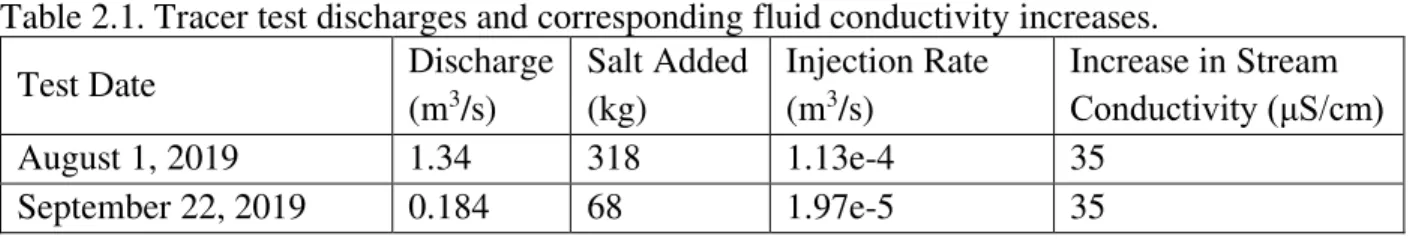
We conducted two four-hour continuous injection salt (NaCl) tracer tests in Cement Creek, one each on August 1 and September 22, 2019 to capture high and low flow in the reach of interest, respectively. The injection site was located 670 m upstream of the measurement site to allow for the salt to mix uniformly in the river water (Figure 2.1). The site was chosen because it provided a relatively even surface to mix the injectate solution, avoided private property lines in the area, and minimized tributary inflows. The tracer was injected at 12:35 pm for the high-flow tracer on August 1, 2019 (Q = 1.34 m3/s) and at 11:59 am for the low-flow tracer on
11
September 22, 2019 (Q = 0.184 m3/s) at constant rates of 1.13e-4 m3/s and 1.97e-5 m3/s, respectively. Measurements of fluid conductivity were taken at the measurement site 670 m below the injection location and upstream of the injection site using a HOBO Conductivity Data Logger (Figure 2.1) at 30-second intervals from 10:00 am the day of the injection to 4:00 pm the day following the injection.
We looked to achieve a 35 μS/cm increase in fluid conductivity in the stream to provide a large enough spike in conductivity to sufficiently differentiate from background levels as tracer migrates through the system (Table 2.1). By injecting the salt at a constant rate for a 4-hour period, the goal was for both the stream fluid conductivity and the bulk conductivity, which is sensitive to the hyporheic zone, to reach a plateau for the duration of the tracer.
Table 2.1. Tracer test discharges and corresponding fluid conductivity increases.
Test Date Discharge
(m3/s) Salt Added (kg) Injection Rate (m3/s) Increase in Stream Conductivity (μS/cm) August 1, 2019 1.34 318 1.13e-4 35 September 22, 2019 0.184 68 1.97e-5 35 2.3.3 Electrical imaging
Electrical resistivity tomography (ERT) was conducted before, during, and after the tracer tests to estimate bulk electrical conductivity in the subsurface by collecting resistance measurements in the field. ERT involves the installation of multiple electrodes along transects of interest, and after inversion of time-lapse data can be used to map tracer transport through the hyporheic zone. An IRIS Syscal Pro was used to make the ERT measurements along a transect perpendicular to flow using a dipole-dipole electrode configuration with 48 electrodes at 1-m spacing, extended 8 m on the left side of the stream and 35 m on the right side into the iron fen (Figure 2.1). The extent of the electrodes installed in the left bank was limited by thick
vegetation at the base of a slope on the left side of the stream. The stream width was 6.7 m during high flow and 5.6 m during low flow. The dipole-dipole configuration was selected for its speed in data collection with a multichannel instrument and its ability to capture lateral changes in conductivity at relatively shallow depths (Alwan, 2013). Each time-lapse survey consisted of 1159 dipole-dipole measurements, or quadripoles. Before the tracer was injected into the stream for the low-flow case, six surveys were measured over two hours to assess the background bulk electrical conductivity of the streambed. Fifty-eight surveys over 27 hours were collected during
12
and after injection to quantify the change in the bulk electrical conductivity from background to capture the transport behavior of the tracer. During high flow, thunderstorms impacted collection of the surveys: three background surveys were collected, six were collected during the tracer test, and thirteen surveys run over 16 hours were taken following the injection.
2.4 Data Analysis Methods 2.4.1 Inversions
The ERT resistance data were inverted using R2 (version 3.3; Binley, 2019). Electrode locations in the model were based off of the topography and spacing of electrodes as measured in the field, and we developed a quadrilateral mesh along the electrode line, extending 100 m in either direction beyond the electrode transect and 100 m in depth, increasing the size of
individual cells with increasing distance from the surface. We conducted time-lapse inversions, which used the background electrical conductivity data and inversion as a starting point for the later inversions. To create the background dataset and inversions, the six backgrounds were averaged. We also input the error for each quadripole measured by the IRIS based on stacked measurements as weights for the inversion.
2.4.2 Analysis of Breakthrough and Hysteresis Curves
In general, the bulk conductivity signal in the hyporheic zone shows longer tails in the subsurface when compared to the fluid electrical conductivity would in the stream (Singha et al., 2008; Ward et al., 2010). Hysteresis curves between bulk conductivity and the co-located fluid conductivity within the stream (Figure 2.2) show the lag in timing between the two, and have been used in previous studies for the evaluation of mass transfer parameters within others system (e.g. Briggs et al., 2014; Briggs et al., 2018).
13
Figure 2.2: (A) Theoretical breakthrough curves for the stream, aquifer, and bulk electrical conductivity; and (B) theoretical hysteresis curve between bulk electrical conductivity and stream electrical conductivity (after Briggs et al., 2014).
To create the bulk and fluid conductivity hysteresis curves, bulk apparent conductivities calculated from the field resistance data were compared against the fluid conductivities measured in the stream water. We applied a geometric factor K to convert each resistance measurement to apparent conductivity, where:
𝐾 = 2𝜋 (𝐴𝑀 −1 𝐵𝑀 −1 𝐴𝑁 +1 𝐵𝑁)1 −1 (2.1) where AM is the distance between injection electrode A and measurement electrode M (m), BM is the distance between injection electrode B and measurement electrode M, etc. To best capture changes from the tracer test within the hyporheic zone, we limited the spacing between
electrodes to 2 m; these quadripoles would be more sensitive to near-surface changes. Apparent bulk conductivity was then calculated by multiplying this geometric factor for each remaining quadripole in the survey by the resistance, which was determined using the injected voltage (V) and measured current (I):
𝜎𝑎 = 𝑉𝐾𝐼 (2.2)
where σa is the apparent bulk conductivity of each quadripole measurement.
The fluid electrical conductivity from the transducer was then plotted against the bulk apparent conductivity at corresponding times. The limbs of the hysteresis curve were then isolated for calculation of the mass transfer parameters using Equations (2.3), (2.4), and (2.5) outlined in Briggs et al. (2014) (Figure 2.2). When performing an analysis based on a hysteresis curve, it is important to have a curve with at least one limb of continuous data and a visible separation between the rising and falling limbs (Briggs et al., 2014). The trends shown in the hysteresis curve (Figure 2.2) associated with a tracer test are explained as follows:
• Points 0→1: The rising limb on the breakthrough curve where both the bulk conductivity and the fluid conductivity increase as the salt from the tracer are introduced to the system. Thus, fluid and bulk conductivity are both increasing, resulting in a positively sloping limb on the hysteresis curve.
• Points 1→2: The fluid conductivity taken in the stream reaches equilibrium and plateaus. The bulk conductivity in the subsurface is still in the process of reaching a plateau as the
14
more sinuous pathways of the aquifer slow the transport of the solute, thus continuing to increase. This time period manifests as an increase in bulk conductivity while
maintaining a constant fluid conductivity, represented by the vertical limb on the hysteresis curve.
• Points 2→3: The tracer injection has finished at this point, resulting in the decrease of conductivity in both the fluid and bulk breakthrough curves.
• Points 3→0: By this point, the salt has left the surface water system and is in the process of leaving the aquifer and reentering the stream, resulting in tailing within the bulk breakthrough curve. The delayed response in the decrease in bulk conductivity should mirror the increase between Points 1 and 2, assuming that the mass transfer parameters remain constant.
Briggs, et al. (2014) calculates the mass transfer parameters α and β from the hysteresis curve: 𝛽 =𝑚𝑚0,2 0,1− 1 = 𝑚0,2 𝑚2,3− 1 = 𝜃𝑖𝑚 𝜃𝑚 (2.3) where mx,y is the magnitude of the slope from Point x to Point y, where x and y represent the specific hinge points as labeled in Figure 2.2; θim represents immobile porosity, and θm represents mobile porosity. In streams, β represents the ratio of the aquifer area to the stream area. Once β is calculated, plotting one of the vertical limbs (from Point 1 to Point 2 or Point 3 to Point 0) as a function of time (t) yields a slope (m) that can provide α:
𝑙𝑛 (𝜎𝜎𝑏,𝑖 − 𝑚0,2𝜎𝑓,𝑖𝑛𝑗
𝑏,0− 𝑚0,2𝜎𝑓,𝑖𝑛𝑗) = 𝑚𝑡 + 𝑏 (2.4)
𝑚 = −𝜃𝛼
𝑖𝑚 (2.5)
where σb,irepresents the bulk conductivity at time step i, σf,inj is the max fluid conductivity at plateau (Points 1 & 2), σb,0 represents bulk conductivity at background (Point 0), and b represents the y-intercept of the line. Once the mass transfer parameters are known, residence times (in seconds) within the less mobile zone can then be calculated, as follows (Fabian et al., 2011):
𝑅𝑒𝑠𝑖𝑑𝑒𝑛𝑐𝑒 𝑇𝑖𝑚𝑒 =𝛽𝛼 .
15 2.4.3 Forward modeling with STAMMT-L
STAMMT-L (version 3.0; Haggerty, 2009) was used to fit mass transfer parameters to the fluid electrical conductivity data. STAMMT-L uses a semi-analytical solution for dual-domain mass transport based on the dual-porosity advection-dispersion equation (ADE). Through iterative forward-model experimentation with α, β, and the dispersivity of the stream (given a known reach length and velocity), we estimated mass transfer parameters which we compared to those calculated from the Briggs method discussed above. By exploring the output from the forward models, we evaluated the effects that each parameter had on the shape of the breakthrough curve. This procedure is outlined in further detail in Appendix A.
For our field measurements and models, we also calculated the Damkohler number (DaI):
𝐷𝑎𝐼 =𝛼(1 + 𝛽)𝐿𝑣 (2.7)
where L represents the length of monitored stream reach (m), α represents the first-order single rate mass transfer between the mobile and less-mobile zones (s-1), β is the capacity coefficient that represents the ratio of immobile storage area to mobile storage area (m2/m2), and v
represents the average velocity of the stream (m/s), as measured when determining the stream’s discharge. Typically, systems with a Damkohler number near 1 will display tailing (Wagner & Harvey, 1997).
2.5 Results & Discussion 2.5.1 Site Observations
Streamflow decreased by an order of magnitude between high (1.34 m3/s) and low flow (0.184 m3/s). The 2019 water year was much wetter than previous years, a result of snowpack well above long-term averages (NRCS, 2020). Between our high- and low-flow
characterizations, iron precipitated along Cement Creek and coated the electrodes used in the geophysical survey (Appendix F). Based on our measurements at Cement Creek near Prospect Gulch and on measurements by the USGS at the outlet of Cement Creek (USGS, 2020), the pH of Cement Creek typically ranges from 3 to 5.
In addition to the decrease in discharge between high and low flows (Table 2.2), there was a corresponding decrease in cross-sectional area and an increase in the concentrations of dissolved metals in the stream; the dissolved aluminum concentrations in the stream increased by 2.34 mg/L during low flow (a 275% increase from high flow) and dissolved iron concentrations
16
increased by 3.87 mg/L (a 98% increase) over the same time (Figure 2.3). This increase in dissolved solids manifested as an increase in fluid EC, with a doubling in background conductivity between high and low flows.
Table 2.2. Stream measurements for high and low flows. Date Streamflow (m3/s) Stream Width (m) Mean Stream Depth (m) Stream Area (m2) pH Temperature (°C) Electrical Conductivity (μS/cm) July 31, 2019 1.34 6.7 0.32 1.6 4.6 8.2 288 September 21, 2019 0.184 5.6 0.12 0.6 3.6 6.2 601
2.5.1 Well Data Indicates Ferricrete Precipitation at Depth
The analyses of the slug tests performed in September and November both indicated a less-permeable layer shallow in the streambed. The heads in the wells at 28-cm and 58-cm depths recovered too quickly using the sounding tape to accurately estimate the hydraulic conductivity. However, the well at 44-cm depth recovered slowly, allowing for measurable changes in hydraulic heads. Three separate slug tests were performed in the 44-cm well, which resulted in a range of results from 7x10⁻⁵ to 2x10⁻⁴ m/s.
The heads measured are consistently lower at 28 cm than at 44 cm (Table 2.3),
corresponded to an upward flow direction for both flows tested. The head within the deepest well did not change significantly (~1 cm difference) with changes in flow and data indicate a
downward flux at high flow and an upward flux at low flow. It is also possible that, as a result of the layer of lower hydraulic conductivity separating these wells, there is limited flow across the 44-cm depth well. It should be noted that we cannot directly quantify the flow between these depths, as we are lacking sufficient information about the hydraulic conductivity of the
uncemented cobbles of the streambed, but it provides a sense of water flow within the hyporheic zone in the specific location of the wells.
Table 2.3: Water heads within the three subsurface wells relative to the surface of the streambed.
Well Depth Head at High Flow (cm) Head at Low Flow (cm)
28 cm 15 8
44 cm 16 9
17
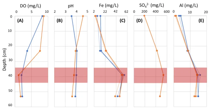
Water chemistry samples from the wells showed higher relative metals concentrations and lower DO in the zone of lower permeability compared to the other wells. According to the study on Cement Creek ferricrete conducted by Wirt et al. (2008), DO in the groundwater is consumed during the formation of sulfate during pyrite dissolution and subsequent oxidation of reduced iron. This would lead to increased concentrations of dissolved iron and sulfate in the groundwater among other metals as is seen in our well data (Figure 2.3). Wirt et al. (2008) investigated the mineral composition of ferricrete along Cement Creek, finding the precipitation of minerals that include schwertmannite (Fe8O8(OH)6(SO4)∙nH2O), potassium jarosite
(KFe3+3(OH)6(SO4)2), and goethite (FeO(OH)). Wirt et al. (2008) also found these minerals to be saturated in the water, resulting in the possibility of precipitation of these ferricrete-forming minerals as well as aluminum-bearing minerals including alunite (KAl3(SO4)2(OH)6) and
gibbsite (Al(OH)3). This is consistent with the high aluminum concentrations near the suspected ferricrete layer, as we found in our groundwater samples at 44-cm depth (Figure 2.3). The iron, sulfate, and aluminum concentrations are highest at the 44-cm depth, and are higher at the 58-cm depth when compared to the stream water and 28-cm depth (Figure 2.3). These increased
concentrations would be expected in an area where ferricrete minerals are supersaturated and might precipitate, as it likely separates the water found in the stream and shallowest well with that in the deepest well. The lower hydraulic conductivity in this ~44-cm layer would also increase the fluid residence time compared to the cobbles above and below, thus allowing for more time for water-sediment interaction and ultimately enhancing the ability for ferricrete to precipitate between the cobbles.
Geochemical modeling performed in PHREEQC showed saturation of iron-sulfate species including jarosite, goethite, and amorphous iron in all three well waters, but higher saturation indices for alunite and jurbanite in the layer of lower hydraulic conductivity (Table 2.3). Alunite and jurbanite are aluminum sulfate minerals formed after the dissolution of sulfide-rich minerals, such as those that can be found in the surrounding San Juan mountains. Jurbanite, specifically, occurs as a post-mining mineral. The supersaturation of alunite and jurbanite in the 44-cm well could potentially account for the precipitation that we saw form on the electrodes and cobble surfaces between high and low flow. We used the x-ray diffraction analyses from Wirt et al. (2008) to inform which ferricrete-forming minerals are commonly found in Cement Creek to
18
include for our interpretation of the saturation index results. Wirt et al. (2008) did not perform analyses of ferricrete at depth, so there might be a larger variety of ferricrete-forming minerals in the subsurface than reported here. Limitations of our analyses include that there may be
sediment-water interactions that were not considered here, surface complexation was not considered, and we used the default equilibrium constants in the WATEQ 4F database for the minerals provided in this analysis, which might not be representative of the environment in which these minerals would precipitate in Cement Creek (Table 2.4). Only high flow was modeled, as the sulfate concentration at low flow was not available; without all of the necessary constituents, the speciation would not accurately reflect saturation levels within the water. Table 2.4: Saturation indices of potential ferricrete-forming minerals, calculated from the geochemical well data (saturation index at high flow/saturation index at low flow). Positive indices represent supersaturation and negative indices represent undersaturation of the mineral in question. Percent error from charge balance as calculated in PHREEQC shown.
K-Jarosite Goethite Fe(OH)3(a) Alunite Jurbanite
Charge Balance (% error) WATEQ 4F log(Keq) -9.21 -1 4.89 -1.4 -3.23 -- Stream 3.57 7.12 1.91 0.13 -0.33 -0.44 28-cm deep well 4.26 5.8 0.25 -2.34 -0.54 5.4 44-cm deep well 6.62 6.9 1.5 0.11 0.11 0.42 58-cm deep well 4.69 5.9 0.59 -2.69 -0.34 4.79
We interpreted the well chemistry results and corresponding modeled saturation indices to represent a layer within the hyporheic zone at 44 cm where ferricrete has deposited and effectively cemented the cobbles together, thereby reducing the hydraulic conductivity. This layer likely formed where the reduced iron in the groundwater is oxygenated by the incoming surface water. Iron concentrations remain high throughout the system, with concentrations that are high enough to supersaturate all waters with many of the solely iron-bearing minerals. As such, the major difference in mineral saturation within the subsurface lies in the aluminum-bearing minerals, which are seen to be supersaturated only at 44-cm depth compared to the other wells. Below this layer at the 58-cm deep well, oxygen concentrations are likely too low for the precipitation of aluminum-bearing minerals that compose ferricrete. For the 28-cm depth, the metals content is lower than the deeper wells (Figure 3c) and the DO concentrations are higher (Figure 3a); thus the aluminum-bearing minerals incorporated in ferricrete would likely not
19
precipitate under these conditions. This reduction in hydraulic conductivity due to heightened iron-oxide precipitation was similarly seen in Vincent et al. with their investigation of Cement Creek (2008). We expect that the depth of hyporheic exchange is largely limited to a depth above 44 cm below the surface, given the lower hydraulic conductivity at that depth and consistent with our STAMMT-L model calculations (Table 2.5).
Figure 2.3: Well water chemistry data from high and low flows shown at the center of the screened depth for the 28-, 44- and 58-cm wells: A) dissolved oxygen concentrations; B) pH levels; C) iron concentrations; D) sulfate concentrations; E) aluminum concentration.
2.5.2 Electrical Inversions Shows Higher Exchange at High Flows and a Laterally Constrained Hyporheic Zone
The averaged background ERT images (Figure 2.4A & F) display consistent zones of high bulk electrical conductivity between high and low flows, especially along the right bank, likely indicative of the iron fen that bounds that side of the stream. In contrast, the left bank is less conductive, as would be expected given the uncemented cobbles that make up the streambed on that side. The bulk electrical conductivity of the streambed itself increases with low flow, given the increase in fluid conductivity discussed before. The thunderstorms occurring
throughout the high-flow tracer test saturated the ground with rainwater, manifesting as higher bulk electrical conductivity along the banks, particularly around the vegetated right bank.
20
The ERT resolution matrices (Figure 2.4E & I) represent how well the model is
constrained by data. Higher resolution is found near the surface. Below about a meter, resolution drops, so the images may be overly smoothed or poorly constrained by data.
Figure 2.4: Electrical inversions looking downstream for high (A-D) and low (F-I) flow regimes, where B-D and G-I represent percent deviation from the background (A, F), with an increase in salinity represented by dark blue. Electrodes 1 through 26 are shown along the stream and banks, as few changes were observed in subsurface conductivity past electrode 27. Rough vegetation extent and iron fen location are also portrayed in top images. (D) and (I) represent the subsurface 16 hours post-injection. (E) and (J) are the resolution matrices, where a log10 value closer to 1 is better constrained by data.
Hyporheic exchange flow is larger during high flow when compared to low flow based on the electrical inversions (Figure 2.4). At high flow, the residence time within the hyporheic
21
zone is comparatively larger, showing increased salinity an hour past when the injection had stopped (Figure 2.4C). In contrast, the low-flow case shows that the system has largely returned to background once the tracer injection had completed (Figure 2.4H). According to the ERT, transport was largely constrained within the upper meter of streambed sediment and did not extend far into either bank. The extent of hyporheic exchange in Cement Creek is small compared to other hyporheic studies, particularly regarding its lateral extent (e.g. Stanford & Ward, 1988; Storey et al., 2003; Ward et al., 2012; Larson et al., 2013; Sparacino, 2017). In sinuous streams, the majority of hyporheic flow extends laterally into stream banks (e.g.
Cardenas & Wilson, 2004; Revelli et al., 2008), though Buffington & Tonina (2009) suggest that lateral flow could also occur in streams with high gradients, such as Cement Creek. However, the right bank of Cement Creek has been cemented together with ferricrete, bounded by an iron fen, and is steeper than the more cobbly, less-cemented left bank (Appendix F). Consequently, it is possible that during high flow, the higher discharge would preferentially flow through the underlying, less-cemented cobbles of the streambed as opposed to the more cemented bank.
Given that ferricrete typically forms from the confluence of oxic and anoxic conditions, the less-permeable layer within the streambed may represent the former vertical extent for hyporheic exchange prior to the precipitation of ferricrete. While the exact depth of this layer cannot be resolved from the inversions alone, the change in chemistry across depth in the subsurface (Figure 2.3), the hydraulic conductivity estimates from slug tests, and the inversion models (Figure 2.4) together suggest that the hyporheic zone of Cement Creek is limited vertically. It is possible that hyporheic exchange has decreased through time as a result of the decreasing permeability from roughly continuous ferricrete deposition. Water would thus likely flow more readily through the uncemented cobbles overlying the layer of ferricrete rather than vertically through the ferricrete layer.
During high flow, the water does not appear to enter into the right bank during the tracer test, though it appears to during the low-flow tracer injection (Figure 2.4B & G). One possible explanation for the increase in bulk electrical conductivity observed in the right bank during the low-flow tracer test could be attributed to the tree roots absorbing water directly from the stream during the tracer test given the comparatively lower soil moisture. This bank was more highly vegetated with trees, and the low-flow tracer test was conducted during the dry season when the ground was comparatively less saturated to the thunderstorm-impacted high-flow system.
22
2.5.3 Mass Transfer Parameter Modeling Indicate a Decrease in Storage Zone Area between High and Low Flows
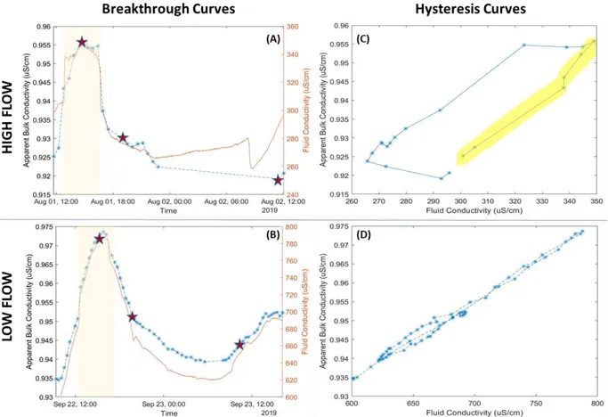
The low-flow relation between the bulk and fluid conductivities for the rising and falling limbs of the breakthrough curve shows little hysteresis (Figure 2.5D), indicating little transient storage in the system. These results correspond with the geophysical inversions that show lower residence within the hyporheic zone during low flow. The high-flow hysteresis curve displays a broader separation, implying hyporheic exchange is present at high flow, as seen in the ERT inversions. Given that the bulk-fluid conductivity hysteresis curves for the tracer tests only displayed separation during high flow (Figure 2.5), the method outlined by Briggs et al (2014) could only be applied for the high-flow case.
As noted earlier, several thunderstorms occurred during the day of the high-flow tracer, resulting in discontinuous breakthrough curves. On the day following the tracer test, the
wastewater treatment plant (Figure 2.1) began to run tests that resulted in shifts in fluid
conductivity that could not be attributed to a natural signal, resulting in the sudden drop in fluid conductivity in the morning. Because of this, the falling limb of the bulk conductivity
breakthrough curve was not captured in detail (Figure 2.5C). Thus, we performed our mass transfer analyses using the rising limb of the hysteresis curve for high flow (Appendix D). To quantify the change in mass transfer parameters between high and low flow, we needed to supplement the hysteresis curve analysis with modeling in STAMMT-L.
When forward modeling solute transport in STAMMT-L, we found that the modeled
concentration breakthrough curves were insensitive to decreases in the mass transfer rate (α) past the threshold of 0.001 s-1 (Table 2.5). Values of α greater than 0.001 s-1 did not fit the measured breakthrough curves as well, providing us with an upper bound for α. The models were more sensitive to the capacity coefficient (β), which is an order of magnitude higher at the high-flow test compared to the low-flow test (Table 2.5), representing larger available storage within the hyporheic zone of Cement Creek. With the larger expected hydraulic heads during the higher discharge, it is possible that water is being forced farther into the hyporheic zone, allowing for access to a larger relative storage zone area. Dispersivity within the model was used as a fitting parameter that affected how smooth the curve appeared. Best-fit dispersivities decreased by an order of magnitude between high and low flow, implying that at high flow the solute spread out as it traveled downstream more than it did at low flow. This follows with the more turbulent flow
23
that occurred at high flow. The modeled breakthrough curves changed with orders of magnitude of variation in β and dispersivity, controlling the smoothing of the curve and controlling arrival of the peak, and were largely insensitive to decreases in α. This indicates that our system is more heavily influenced by relative storage area within the hyporheic zone and dispersivity. More on the sensitivity to these parameters can be found in Appendix C.
Figure 2.5: Fluid and bulk conductivity breakthrough curves (A & B) and associated hysteresis curves (C & D) for high- and low-flow tracer tests. Stars on the bulk conductivity breakthrough curves represent times of the inversions represented in Figure 2.4. Beige rectangles in A & B represent the timing of the tracer injections. The highlighted limb in C represents the limb used for the mass transfer parameter analysis outlined in Briggs et al. (2014).
The α and β parameters from the graphical analysis are consistent with those from the best-fit STAMMT-L model for the high flow tracer test (α was found to be 0.001 in STAMMT-L and 0.0012 from the hysteresis curve; β was 0.3 in STAMMT-L and 0.3 from the hysteresis curve) (Table 2.6). To graphically compare both models, the mass transfer parameters found with the analysis of the high flow hysteresis curve were input into STAMMT-L to simulate a
24
breakthrough curve (Figure 2.6). The modeled breakthrough curves show a reasonable match (RMSE < 15%) for the measured fluid conductivity breakthrough, but miss the elevated
concentrations in the tail. The fluid conductivity data were more variable than the model results given field variability in pumping rates, streamflow rates, and injected concentration. While we did our best to note these, several branching tributaries also flow into Cement Creek (Figure 2.1), whose inflows and relative fluid conductivities were not accounted for when correcting the electrical conductivity data at our measurement site for background electrical conductivity. While it is possible that inflows near draining mines could influence the breakthrough curves, the shift that would result from these inflows should not have an influence as large as what is seen in Figure 2.6, given their relatively small flows compared to the overall flow of Cement Creek (flow through Prospect Gulch is likely ~10% of Cement Creek’s flow).
Table 2.5: Parameters used for best-fit models in STAMMT-L for high and low flow, and parameters found with the Briggs et al. (2014) hysteresis curve analysis.
Parameter High-Flow Hysteresis High Flow STAMMT-L Low Flow STAMMT-L Velocity (m/s)* 0.831 0.831 0.239 Dispersivity (m) 67 67 6.7 α (1/s) 0.0012 0.001 0.001 β (-) 0.3 0.3 0.01 Damkohler Number (-) 1.3 1.1 2.8
Stream Channel Area (m2)* 1.6 1.6 0.6
Transient Storage Area (m2) 0.48 0.48 0.0062
Residence Time (s) 250 300 10
* Parameters measured in the field.
It is possible that the ferricrete precipitation alters our system such that it cannot be modeled with solely two domains (the stream and the subsurface) connected by 1-D flow, as conceptualized in the numerical model. The slug test data suggest that the ferricrete layer is less permeable than the cobbles, but not completely impermeable. Thus, diffusion between the cobbles and the underlying ferricrete layer could result in longer retention of the solute within the ferricrete. This solute would re-enter the stream at a slower rate than the solute traveling through the cobbles, resulting in an increased fluid conductivity in the tail that would not be represented in the rising limb. The effect is more prominent at high flow than at low flow, as seen by the tail reaching 35% of the maximum conductivity at that time, as opposed to about
25
15% of maximum conductivity at low flow. Consequently, we can either fit the rising limb and plateau, or solely fit the tail (Appendix C, Test 2-14). As such, most of the emphasis in the STAMMT-L analysis presented here was placed on the arrival and rising limbs and the timing of the falling limbs. We matched the arrival time of the tracer at the measurement site using the measured velocity and experimentally changed the dispersivity of the stream for both flow regimes individually. The slopes of the rising and falling limbs were matched by altering the mass transfer rate and capacity coefficients for the best fit visually. The root mean square error (RMSE) test between modeled versus observed electrical conductivity values allowed for quantification of this fit once the final mass transfer parameters had been finalized (Table 2.6, Appendix E).
Figure 2.6: Modeled and field fluid conductivity breakthrough curves for (A) high- and (B) low-flow tracer tests. The green rectangles represent the rising limbs used to create (C); the orange rectangles represent the falling limbs used to create (D). The stars in (C) represent the times at which the rising limbs reach plateau.
26
The breakthrough curve created with the calculated mass transfer parameters estimated from the Briggs method also match the arrival and departure timing of the field measurements reasonably well, within 15% error (Figure 2.6). While the model created using the mass transfer parameters from the bulk-fluid conductivity hysteresis curve did not capture the gradual rise to the plateau as well as the STAMMT-L model does, it otherwise shows the same trends observed from the other analyses, where high flow displays more solute retention, indicative of longer residence times within the hyporheic zone. To provide the best comparison between the
STAMMT-L and predicted breakthrough curves from the hysteresis curve parameters, we kept the dispersivity between the two constant at 67 m, as the hysteresis curve method did not provide a manner with which to calculate dispersivity directly.
The rising limb of low-flow breakthrough curve breaks through roughly 90 minutes before and reaches plateau sooner than the high-flow rising limb (Figure 2.6C). This was quantified directly through residence time, which decreased by an order of magnitude between high and low flow (Table 2.5). These results are consistent with the geophysical inversions, which display more solute in the subsurface during high flow post-injection (Figure 4c). Further smoothing of the breakthrough curves and increased tailing at late time would be expected where retention is more prominent.
Table 2.6. RMSE values for model fits for full breakthrough curves and portions without tailing.
Test RMSE, full BTC RMSE, no tail
High Flow, STAMMT-L 20.0% 6.8%
High Flow, Hysteresis 21.2% 8.2%
Low Flow, STAMMT-L 13.4% 12.4%
We compared the RMSE between the model-predicted fluid conductivity and observed fluid conductivity values to quantify how well the models fit the observed data. We calculated the RMSE for both the entire breakthrough curve and the portion of the breakthrough curve before the tails (Table 2.6, Appendix E). Without including the tailing in the falling limb, errors were below 15%. The low-flow case is less sensitive than the high-flow case to the elevated electrical conductivity post-injection because the normalized high-flow fluid conductivity in the tail was twice as large as the low-flow tail. The majority of the error in the high-flow models arises from the minor offset in timing of the falling limb, while the error in the low-flow model can be attributed to the offset in the magnitude of the plateau values.
27 2.6 Conclusions
Our findings indicate that a ferricrete-impacted river has limited hyporheic exchange, especially at lower flows, as conceptualized by Figure 2.7. Without ferricrete, the streambed of Cement Creek could support an extensive hyporheic zone, given the rough surface layer of cobbles; however, iron precipitation reduces the hydraulic conductivity of the streambed, acting as a barrier for water and limiting the level of mixing between the surface water and the
groundwater. Exchange is limited to the upper tens of centimeters of the streambed based on the layer of low hydraulic conductivity found from the slug tests and the small estimates of transient storage area at both high and low flow from the breakthrough curve modeling. Geochemistry of the water samples in the streambed were consistent with the precipitation of ferricrete, showing high iron, sulfate, and aluminum concentrations at 44-cm when compared to the 28-cm and 58-cm depths.
Our ERT maps delineate a laterally and vertically constrained zone of exchange, likely due to cementation along the banks and beneath the surface. Exchange between the stream and the hyporheic zone becomes particularly limited at low flows. This result was supported in both the STAMMT-L models and the mass transfer parameters calculated directly from the field measurements using the Briggs method, where we found higher residence times at high flow (300 s) compared to low flow (10 s), implying that the higher discharge drives hyporheic exchange in Cement Creek. The streambed appearance remained relatively unchanged between the two tests, except for a thin layer of cementation noted between tests, suggesting that changes in flow are what primarily affected the extent of hyporheic exchange as opposed to relative topographical features along the streambed.
Cement Creek is subject to notable pollution from the upstream draining mine adits, making the pollution attenuation potential from hyporheic exchange important to the water quality of the stream. However, there is reduced exchange during low flow when solute
concentrations are highest. Rather, exchange is more notable at higher flows when contaminant concentrations are much lower, thereby limiting natural pollution filtration of Cement Creek. This implies that the hyporheic zone of Cement Creek might not be an effective filter for metals sequestration and corresponding pollutant attenuation at these times. Instead, it is possible that concentrations of contaminants from events like the Gold King Mine spill would be mitigated from natural dilution rather than filtration from the hyporheic zone. The heterogeneous nature of