Capacity and Cell-Range Estimation
for Multitraffic Users
in
Mobile WiMAX
Amir Masoud AHMADZADEH
This thesis comprises 30 ECTS credits and is a compulsory part in the Master of Science with a Major in Electrical Engineering – Communication and Signal Processing , 181 – 300 ECTS credits
Capacity and Cell-Range Estimation for Multitraffic Users in Mobile WiMAX
Amir Masoud AHMADZADEH am_ahmadzadeh82@yahoo.com
Master thesis
Subject Category: Wireless Communication Technology Series and Number Electrical Engineering – 2/2008
University College of Borås School of Engineering SE-501 90 BORÅS
Telephone +46 033 435 4640
Examiner: Jim Arlebrink
Supervisor: Dr. Jose Antonio Portilla Figueras antonio.portilla@uah.es
Client: Universidad de Alcalá Escuela Politécnica Superior 28871- Alcalá de Henares (Madrid) Tel: +34 91 8856504
Date: September 2008
Keywords: mobile wimax , IEEE802.16 , capacity estimation , mixed user traffic
Acknowledgment :
I would like to express my deep appreciation to my advisor, Dr. Jose Antonio Portilla- Figueras, for his direction and guidance. Thank you for being so helpful and friendly all the times, beside educational matters.
Special thanks to Mr. Antonio Guerrero Baquero. He explicitly bears a great portion of helping me to get the chance to follow my interests.
I also wish to have a reminder of my colleagues at the company of Telefónica I+D for their assistance in finding useful reference information.
Finally, the words alone cannot express the thanks I owe to my parents for their all-out support and to Cristina for her tender friendship.
September 2008 Amir M. Ahmadzadeh
Abstract:
The fundamentals for continued growth of broadband wireless remain sound. According to the Ericsson’s official forecasts, the addressable global market of wireless internet broadband connectivity reaches to 320 million users by the end of 2010. The opportunity for BWA/WiMAX to serve those who want to switch to broadband service is huge in many parts of the world where wireline technologies may not be feasible.
The current document (Capacity and Cell-range Estimation for Multitraffic Users in Mobile WiMAX) is prepared as a master’s program final thesis to peruse the service provision capabilities of Mobile WiMAX innovate technology in more details. An elaborate excerpt of the technical subjects of IEEE-802.16e-2005 standard is gathered in the first chapter to provide the reader with a practical concept of Mobile WiMAX technology. The following chapter is aimed to collect the required knowledge for WiMAX planning problem. An innovate methodology to calculate the system’s actual throughput and a traffic model for mixed application users are proposed with a step by step description to derive an algorithm to determine the maximum number of subscribers that each specific Mobile WiMAX sector may support. The report also contains a Matlab code –enclose in the appendix– that tries to implement the entire algorithm for different system parameter and traffic cases to ease the Mobile WiMAX planning problem. The last chapter introduces the mostly used propagation models that suit the WiMAX applications.
The presented methodology would help those operators that plan to implement a wide coverage network in a city. Using the introduced methodology, service providers will be able to estimate the number of base stations and hence the network investment and profitability.
Contents :
Acknowledgment………... iii Abstract………. iv Acronyms………... vii List of Tables………. ix List of Figures………... xChapter1: Technical Overview of Mobile WiMAX
1.1- Introduction……… 11.2- Wireless Channel Overview………... 2
1.3- Physical Layer……… 5
1.3.1- OFDM……….. 5
1.3.2- OFDMA………... 6
1.3.3- SOFDMA……… 7
1.3.4- Channel Modulation and Coding………. 9
1.3.5- Frame Structure………... 10
1.4- MAC Layer………. 13
1.4.1- MAC Layer Structure……….. 13
1.4.2- MAC PDU Structure………... 14
1.4.3- Bandwidth Allocation……….. 15
1.4.4- Quality of Service (QoS) and Scheduling………... 15
1.4.5- Mobility Management………. 16
1.4.5.1- Power Control………... 16
1.4.5.2- Handoff………. 17
1.5- Throughput and Coverage……….. 18
1.5.1- Throughput and Data rate……… 18
1.5.2- Coverage and Cell Range……….20
1.5.3- Adaptive Modulation and Coding technology………. 22
References……….. 23
Chapter 2: Capacity Analysis of Mobile WiMAX
2.1- Introduction……… 242.2- Modulation Distribution………. 25
2.3- Application Distribution………. 28
2.3.1- Service Flows……….. 28
2.3.2- Applications Parameters……….. 30
2.3.3- Traffic and QoS Control Modeling………. 31
2.3.3.1- Contention Ratio………... 31
2.3.3.2- Over Subscription Ratio………... 32
2.3.4- Application Distribution and Market Trends…………... 33
2.4- Useful bandwidth estimation……….. 37
2.4.1- Downlink………. 38
2.4.2- Uplink……….. 43
2.5- Maximum User per Sector Determination……….. 47
References……….. 49
Chapter 3: Propagation Models for BWA
3.1- Introduction……… 503.2- SUI Model……….. 50
3.3- Cost-231 Hata Model……….. 52
3.4- Comparison of Propagation Models………... 53
References……….. 54
Appendix 1………. 55
Appendix 2………. 61
Future Work……….. 69
Acronyms :
3GPP 3G Partnership Project AAS Adaptive Antenna System
AMC Adaptive Modulation and Coding ATM Asynchronous Transfer Module BE Best Effort
BPSK Binary Phase Shift Keying BRH Bandwidth Request Header BS Base Station
BW Bandwidth
BWA Broadband Wireless Access CBR Constant Bit Rate
CC Convolutional Coding CID Connection Identifier CP Cyclic Prefix
CQICH Channel Quality Indicator CR Contention Ratio CRC Cyclic Redundancy Check CS Convergence Sublayer CTC Convolutional Turbo Coding DAC Digital to Analogue Converter DCD Downlink Channel Descriptor DIUC Downlink Interval Usage Code
DL Downlink
FBSS Fast Base Station Switching FCH Frame Control Header FDD Frequency Division Duplex FEC Forward Error Correction FFT Fast Fourier Transform FRF Frequency Reuse Factor FTP File Transfer Protocol FUSC Fully Used Sub-Carrier GM Grant Management GMH Generic MAC Header
GSM Global System for Mobile communications HARQ Hybrid Automatic Repeat Request
HHO Hard Hand-Off
HSPA High Speed Packet Access HTTP Hyper Text Transfer Protocol IE Information Element
IEEE Institute of Electrical and Electronics Engineers IP Internet Protocol
ISI Inter-Symbol Interference LOS Line Of Sight
LTE Long Term Evolution MAC Medium Access Control MAP Media Access Protocol MAU Minimum Allocation Unit MDHO Macro Diversity Hand Over MIMO Multiple Input Multiple Output MS Mobile Station
NF Noise Figure NLOS Non Line-of-Sight OCR Overall Coding Rate
OFDM Orthogonal Frequency Division Multiplex OFDMA Orthogonal Frequency Division Multiple Access OSR Over Subscription Ratio
P2P Peer to Peer PDU Packet Data Unit PHY Physical Layer Protocol PL Path Loss
PUSC Partially Used Sub-Carriers QAM Quadrature Amplitude Modulation QoS Quality of Service
QPSK Quadrature Phase Shift Keying RF Radio Frequency
RSSI Received Signal Strength Indicator SDU Service Data Unit
SIMO Single Input Multiple Output SNIR Signal to Noise + Interference Ratio SNR Signal to Noise Ratio
SOFDMA Scalable Orthogonal Frequency Division Multiple Access SS Subscriber Station
SUI Stanford University Interim TDD Time Division Duplex
TDM Time Division Multiplexing UCD Uplink Channel Descriptor UE User Equipment
UL Uplink
UMTS Universal Mobile Telephone System
UTRAN Universal Terrestrial Radio Access Network VBR Variable Bit Rate
VoIP Voice over IP
WiMAX Worldwide Interoperability for Microwave Access
List of Tables :
Table 1.1 OFDM symbol parameters for Fixed and Mobile WiMAX
Table 1.2 Uplink and Downlink Burst Profile in IEEE 802.16e-2005
Table 1.3 Mobile WiMAX Service Flows and QoS parameters
Table 1.4 Mobile WiMAX Frequency parameters
Table 2.1 Modulation and coding supported in Mobile WiMAX
Table 2.2 Minimum Receiver Sensibility for different Modulation and Coding
Table 2.3 Modulation Distribution Assumption
Table 2.4 Application Distribution Assumption
Table 3.1 Numerical values for the SUI model parameters
Table 3.2 Cost-231 Hata model limitations
Table 3.3 Statistical Comparison of Propagation Models
List of Figures :
Figure 1.1 Wireless channel model
Figure 1.2 Three different wireless channel’s trends
Figure 1.3 OFDM Symbol Structure with Cyclic Prefix
Figure 1.4 Frequency domain representation of OFDMA symbol
Figure 1.5 OFDM and OFDMA channel allocation in uplink
Figure 1.6 WiMAX OFDMA TDD Frame Structure
Figure 1.7 Frequency Reuse Implementation in Sectoring
Figure 1.8 WiMAX MAC layer
Figure 1.9 MAC PDU Structure
Figure 1.10 Global percentage of WiMAX deployments per frequency band
Figure 1.11 Adaptive Modulation and coding Figure 2.1 Channel bandwidth partitioning
Figure 2.2 Global WiMAX Deployment by End-user Type
Figure 2.3 Application Distribution of a European UMTS-HSPA service operator
Figure 2.4 Downlink useful bandwidth calculation algorithm
Figure 2.5 Packing and Fragmentation Techniques in WiMAX
Figure 2.6 Uplink useful bandwidth calculation algorithm
Figure 2.7 Maximum Number of Users per Sector Calculation Algorithm
Chapter 1
Technical Overview of Mobile WiMAX
1.1- Introduction:
The first specification of Metropolitan Area Wirless Network was approved under the IEEE 802.16 standard with product certification name of WiMAX. The IEEE 802.16-2004 standard was developed to add NLOS applications support to the basic standard. This standard serves fixed and nomadic users in the frequency range of 2 – 11 GHz. In order to add mobility to wireless access, the WiMAX, IEEE 802.15e-2005 specification was defined, utilizing frequencies below 6 GHz.
There are multiple physical-layer choices, within IEEE 802-16 standard. Similarly, there are multiple choices for MAC architecture, duplexing, frequency band of operation, etc. In fact, one could say that IEEE 802.16 is a collection of standards, not one single interoperable standard. To grant interoperability the WiMAX Forum defines a limited number of system profiles and certification profiles. A System Profile defines the subset of mandatory and optional physical and MAC-layer features selected by the WiMAX Forum from the IEEE 802.16-2004 or IEEE 802.16e-2005 standard. By now two different system profiles are defined : one based on IEEE 802.16-2004, OFDM PHY, called the fixed system profile; the other one based on IEEE 802.16e-2005 scalable OFDMA PHY, called the mobility system profile. The Mobile WiMAX standard has been developed to be the best wireless broadband standard for portable devices enabling a new era of high throughput and high delivered bandwidth together with exceptional spectral efficiency when compared to other 3G+ mobile wireless technologies
In this chapter the fundamental technical aspects of WiMAX are elaborated with a focus on Mobility System Profile. Comparisons between two different system profiles are made, whenever needed, to help a better understanding.
1.2- Wireless Channel Overview:
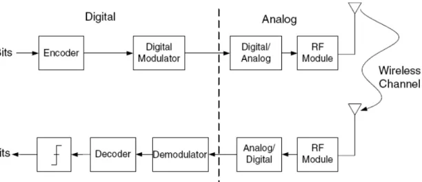
A wireless channel can be modeled as Figure 1.1.
Figure 1.1- Wireless channel model
The transmitter receives packets of bits from a higher protocol layer and sends those bits as electromagnetic waves toward the receiver. The key steps in the digital domain are encoding and modulation. The encoder generally adds redundancy that will allow error correction at the receiver. The modulator prepares the digital signal for the wireless channel and may comprise a number of operations. The modulated digital signal is converted into a representative analog waveform by a digital-to-analog convertor (DAC) and then upconverted to one of the desired WiMAX radio frequency (RF) bands. This RF signal is then radiated as electromagnetic waves by a suitable antenna. The receiver performs essentially the reverse of these operations.
There are 3 major factors affecting wireless channels that can not be found in wired networks. These are Pathloss, shadowing and fading. Each of these phenomena impact the received signal in a especial manner.
Pathloss refers to the reduction of the energy between transmitter and receiver that are
located at a distance d away from each other. This concept is dependent on the
propagation environment. There are different formulas suggested for pathloss calculation in different urban, suburban and rural environments. Pathloss is the base of cellular network designs.
Shadowing can be caused by obstacles that are located between transmitter and receiver
that affect the received power. On the other words, any abnormal changes in the amount of received power in both degrading or increasing way, for example absorption or diffraction caused by a building or a temporary line-of-sight transmission path, is referred to as shadowing.
Unlike pathloss or shadowing that are large scale attenuation effects owing to distance or obstacles, fading is caused by the reception of multiple versions of the same signal. These multiple versions referred as multipath between Tx and Rx can arrive at the receiver at nearly the same time. In this case, depending on their phase difference, the interferences can be constructive or destructive when being combined.
The fading characteristic of wireless channels is perhaps the most important difference between wireless and wired communication system design. The other most notable differentiating factors for wireless are that all users nominally interfere with one another in the shared wireless medium and that portability puts severe power constraints on the mobile transceivers
The fundamental function used to statistically describe broadband fading channels is the two-dimensional autocorrelation function A(Δτ,Δt)
A(Δτ,Δt) = E [h( τ1,t1 ) h*( τ2,t2 )] (eq-1.1)
Where h(.) is the channel response that is variant in two dimensions: delay τ , time t . The channel spread delay is normally the duration of this aforesaid channel response denoted as τmax. The corresponding frequency domain value is called coherence bandwidth, BBc
which is the range of frequencies over which the channel remains constant.
Bc = 1 / τmax (eq-1.2)
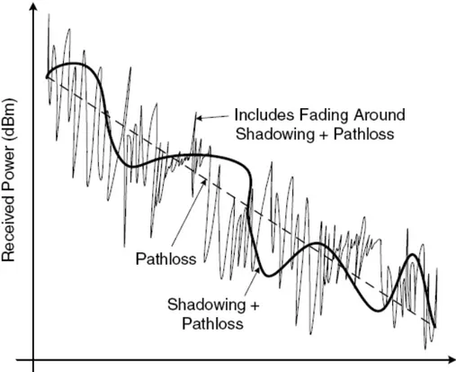
Figure 1.2 compares different wireless channel effects on the received power as the
distance between Tx and Rx increases.
Figure 1.2- Three different wireless channel’s trends
As can be seen in the figure, in general, fading is time varying (fluctuant) signal amplitude attenuation and shadowing that is a consequence of signal absorption by the obstacles in the terrain between the BS and UE, causes a variance around the distance dependent mean pathloss.
1.3- Physical Layer:
In this section the supported access provision air interface technologies for different WiMAX profiles are elaborated.
1.3.1- OFDM:
The WiMAX physical layer is based on Orthogonal Frequency Division Multiplexing. OFDM is the transmission scheme of choice to enable high-speed data communications in broadband systems. OFDM belongs to a family of transmission schemes called
multicarrier modulation, which is based on the idea of dividing a given high-bit-rate data
stream into several parallel lower bit-rate streams and modulating each stream on separate subcarriers. This technique helps us with minimizing the Intersymbol
Interference (ISI). The number of substreams is chosen to ensure that each subchannel has a bandwidth less than the coherence bandwidth of the channel, so the subchannels experience relatively flat fading.
In order to keep each OFDM symbol independent of the others after going through a wireless channel, it is necessary to introduce a guard time, Tg, between OFDM symbols. This way, after receiving a series of OFDM symbols with duration Ts, as long as the guard time is larger than the delay spread of the channel, each OFDM symbol will interfere only with itself.
In order to completely eliminate the ISI and benefit a ISI-free channel Cyclic Prefix technique is used. Figure 1.3 explains the concept of CP. The ratio of cyclic prefix to useful symbol time is indicated by G and can undertake values of 1/4 , 1/8 , 1/16 or 1/32 .
Figure 1.3 - OFDM Symbol Structure with Cyclic Prefix
1.3.2- OFDMA:
The total capacity available with a base station is shared among multiple users on a demand basis, using a burst TDM scheme. When using the OFDMA-PHY mode, multiplexing is additionally done in the frequency dimension, by allocating different subsets of OFDM subcarriers to different users. This is done based on subchannelization method.
Subchannelization is the method that differentiates OFDMA with OFDM. The available
subcarriers within the total bandwidth can be divided into several groups of subcarriers called subchannels. Subchannels can be assigned to the users on a logical procedure based on user demands and channel conditions. OFDMA is essentially a hybrid of FDMA and TDMA: Users are dynamically assigned subcarriers (FDMA) in different time slots (TDMA).
There are 4 different types of subcarriers in an OFDMA symbol. Data subcarriers and
Pilot subcarriers (used for estimation and synchronization purposes). These two first
types are considered Active subcarriers. DC subcarriers together with Guard subcarriers (used for guard bands) are commonly denominated as Null subcarriers. Figure 1.4 illustrates the OFDMA symbol’s subcarrier structure.
Figure 1.4 - Frequency domain representation of OFDMA symbol
The number and exact distribution of the subcarriers that constitute a subchannel depend on the subcarrier permutation mode. A distributed subcarrier permutation draws subcarriers pseudo-randomly to form a subchannel and provides better frequency
diversity, whereas an adjacent subcarrier distribution allows the system to exploit multiuser diversity. In general, distributed (diversity) permutations perform well in mobile applications while adjacent (contiguous) permutations are well appropriated for fixed, portable or low mobility environments.
In order for each MS to know which subcarriers are intended for it, the BS must broadcast this information in downlink MAP messages.
Figure 1.5 reveals a graphical comparison between OFDM and OFDMA considering 4
different users sharing same bandwidth in both techniques in the uplink.
Figure 1.5 - OFDM and OFDMA channel allocation in uplink
1.3.3- SOFDMA:
The mobile WiMAX - IEEE 802.16e-2005, is based on Scalable Orthogonal Frequency Division Multiple Access. The available bandwidth for WiMAX can vary based on the local frequency usage over the globe and the scalability is developed to support these worldwide variations. Therefore SOFDMA refers to the capability of choosing the number of subcarriers according to the available bandwidth. The channel bandwidth can vary from 1.25 MHz to 20 MHz and thus, a number of 128 to 2048 subcarriers can be assigned to each bandwidth correspondingly.
Table 1.1 summarizes the OFDM symbol parameters for Fixed WiMAX (IEEE
802.16-2004) and the equivalent OFDMA symbol parameters used in Mobile WiMAX (IEEE 802.16e-2005) in downlink direction. The diverse values for parameters in OFDMA refer to the scalability concept.
.Table 1.1 - OFDM symbol parameters for Fixed WiMAX and the equivalent OFDMA symbol parameters used in Mobile WiMAX in downlink.
As can be observed in Table 1.1, the subrcarrier distribution for Mobile profile is derived with respect to PUSC permutation mode that is the mandatory resource grouping method in IEEE 802-16e standard. In this permutation mode, the DL usable sub-carriers (pilot and data) are grouped in clusters where each cluster contains 14 contiguous sub-carriers per symbol. Each cluster will be integrated by 12 data carriers and 2 pilot sub-carriers. So as an example in 5MHz channel since we have 360 data sub-carriers and 60 pilot subcarriers, there will be (360+60)/(12+2)=30 clusters. In addition, each sub-channel is composed by 2 clusters, so there will be 30/2 = 15 subsub-channels in DL PUSC. The standard also defines FUSC (Fully Used Sub-Carriers) as an optional alternative permutation mode.
1.3.4- Channel Modulation and Coding:
The mandatory coding scheme used in IEEE 802-16e is Convolutional Coding , CC. Several optional encoding methods such as turbo coding and low density parity check coding are also defined in the standard. Different coding rates of ½ and ¾ can be used within the coding stage with respect to DL and UL.
After encoding, the next step is interleaving. The encoded bits are interleaved using a two step process. The first step ensures that the adjacent coded bits are mapped onto nonadjacent subcarriers, which provides frequency diversity and improves the performance of the decoder. The second step ensures that adjacent bits are alternately mapped to less and more significant bits of the modulation constellation.
During the symbol mapping stage, the sequence of binary bits is converted to a sequence of complex valued symbols. The mandatory constellations are QPSK and 16-QAM, with an optional 64-QAM constellation. Higher modulation levels provide higher data rates. These tones are used to modulate the subcarriers and will form the subchannels based on the subcarrier permutation mode. The number of subchannels allocated for transmitting a data block depends on various parameters, such as the size of the data block, the modulation format, and the coding rate.
The overall information about the transmitted data will be presented in a burst profile. The burst profile provides the receiver with information like : modulation type, channel coding rate, coding and error correction schemes. There are 52 different burst profiles defined in IEEE 802.16e-2005 that can be reviewed in Table 1.2.
Table 1.2 - Uplink and Downlink Burst Profile in IEEE 802.16e-2005
1.3.5- Frame Structure:
In IEEE 802.16e-2005, both frequency division duplexing and time division duplexing are allowed. In the case of FDD, the uplink and downlink subframes are transmitted simultaneously on different carrier frequencies; in the case of TDD, the uplink and downlink subframes are transmitted on the same carrier frequency at different times. It should be noted that all the current candidate mobility profiles are TDD based. That is because of TDD’s higher efficiency in asymmetric traffic: most of the times downlink occupies a higher ratio of the total frame. The TDD WiMAX frame is divided into 2
subframes for DL and UL. These two subframes are separated with a transmission gap.
Figure 1.6 illustrates the TDD frame structure of WiMAX.
Figure 1.6 - WiMAX OFDMA TDD Frame Structure
The first OFDM symbol in the downlink subframe is used for transmitting the DL
preamble that is used for a variety of PHY layer procedures, such as time and frequency
synchronization, initial channel estimation, and noise and interference estimation. Frame
Control Header (FCH) specifies the some characters of the bursts such as length and
number of the bursts. The DL MAP and UL MAP introduce the channel allocation information that are broadcasted to all users. Listening to MAP messages each user can identify the data region (sub-carriers) allocated for its use in both DL and UL. Each DL
data burst is assigned a burst profile and contains the data for an individual user.
The ranging in the uplink is done to assure a reliable communication by performing time and power synchronization. Bandwidth request with the users may be followed by ranging symbols. Then the users transmit in each UL data Burst within their allocated subcarriers, already known by UL MAP. The Uplink Channel Quality Indicator (CQICH) is allocated to feedback channel state of each terminal to the BS’s scheduler to be used for AMC as an example. The ACK uplink channel is the downlink HARQ acknowledgment.
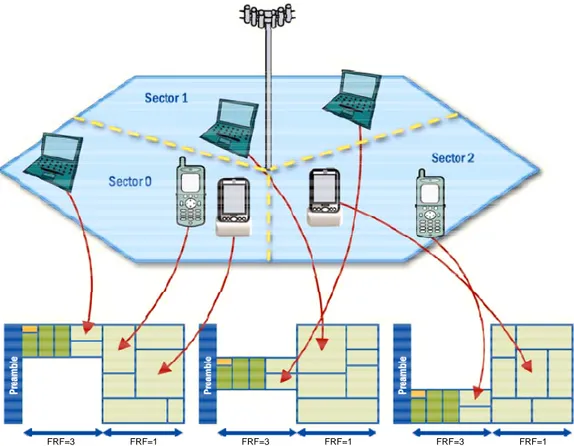
Since the OFDMA PHY layer has many choices of subcarrier allocation methods, multiple zones can use different subcarrier allocation methods to divide each subframe. One benefit of using zone switching is that different frequency reuse factors (FRF) can be deployed in a cell or sector, dynamically. Figure 1.7 shows an example of deploying different FRFs in one frame. For the first half of each frame, the entire frequency band is divided by three and allocated in each sector. For the second half of each frame, the whole same frequency band is used in each sector. The benefits of deploying different FRFs in one frame are: (1) the FCH and DL-MAP are highly protected from severe co-channel interference; (2) edge users, who are receiving co-co-channel interference from other sectors in other cells, also have suppressed co-channel interference; and (3) users around the cell center have the full frequency band because they are relatively less subject to co-channel interference.
FRF=3 FRF=1 FRF=3 FRF=1 FRF=3 FRF=1 Sector 1 Sector 2 Sector 3
Figure 1.7- Frequency Reuse Implementation in Sectoring
1.4- MAC Layer:
In WiMAX technology, second network layer plays some critical roles in the specification such as packeting and fragmentation, channel allocation, scheduling, QoS and security provision and finally mobility management. In this section the MAC layer’s entity and tasks are mentioned.
1.4.1- MAC Layer Structure:
The WiMAX MAC layer consists of 3 sublayers as it is revealed in Figure 1.7.
Figure 1.7 - WiMAX MAC layer
The Convergence Sublayer , CS, that treats as the interface between any higher layers
above MAC layer and its lower sublayers. CS receives higher layer packets also known as Service Data Units, SDU, and maps them into appropriate forms for further processes within MAC layer, such packet address identifications. Whereas both ATM and IP connotations are defined in the IEEE 802.16e standard, WiMAX Forum has decided to implement only IP services.
MAC common part sublayer is responsible for receiving SDUs and applying appropriate
fragmentation and concatenation over them , forming MAC PDUs , Protocol Data Units, and preparing PDUs for transmission. Based on the size of the payload, multiple SDUs can be carried on a single MAC PDU, or a single SDU can be fragmented to be carried over multiple MAC PDUs. Quality of service, QoS, control channel allocation and scheduling are other tasks made in this sublayer.
MAC Security Sublayer ,as the name implies , handles security tasks such as
authentication and encryption.
1.4.2- MAC PDU Structure:
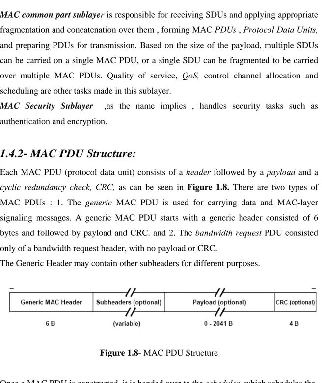
Each MAC PDU (protocol data unit) consists of a header followed by a payload and a
cyclic redundancy check, CRC, as can be seen in Figure 1.8. There are two types of
MAC PDUs : 1. The generic MAC PDU is used for carrying data and MAC-layer signaling messages. A generic MAC PDU starts with a generic header consisted of 6 bytes and followed by payload and CRC. and 2. The bandwidth request PDU consisted only of a bandwidth request header, with no payload or CRC.
The Generic Header may contain other subheaders for different purposes.
Figure 1.8- MAC PDU Structure
Once a MAC PDU is constructed, it is handed over to the scheduler, which schedules the MAC PDU over the PHY resources available. The scheduler determines the optimum PHY resource allocation for all the MAC PDUs, on a frame-by-frame basis. Based on the traffic class, the scheduler can assign the whole frame or a single time slot to a terminal. It is good to note that WiMAX is designed to support all different traffic modules out of 4 different existing ones. These are : Background (messages) , Interactive (web browsing) , Streaming (video) and Conversational (VoIP) in delay sensitivity increasing order.
1.4.3- Bandwidth Allocation:
In the downlink, all decisions related to the allocation of bandwidth to various MSs are made by the BS without the involvement of the MS based on CID, Connection Identifier. These CIDs are 16-bit addresses used to distinguish between multiple UL channels (connections) associated with the same DL channel. The Mobile Stations or Subscriber Stations, SS, check CIDs in the received PDUs and retain only those PDUs that are addressed to them. As mentioned before, the PHY recourses allocated for PDU transmission in each connection is indicated in DL-MAP messages.
In the uplink, the MS requests resources by using a bandwidth request subheader on a MAC PDU. The BS allocates dedicated (intended for a single SS) or shared (intended for a group of SSs) resources for the users periodically which can be used to request bandwidth. In WiMAX this process is called Polling.
1.4.4- Quality of Service (QoS) and Scheduling :
Each user can achieve the desired bandwidth based on the Quality of service that is defined for it. The system should grant a reliable connection based on the agreed QoS parameters within a connection. A key concept in QoS is Service Flow. Each service flow or category is associated with a unique set of QoS parameters, such as latency, jitter throughput, and packet error rate, that the system strives to offer. Table 1.3 illustrates service flows supported in Mobile WiMAX and gives example applications for each. Before providing any certain type data service, the BS’s MAC establishes an unidirectional connection with its peer MAC layer in the user terminal to discuss the agreed service flow and assign the QoS parameters over the air interface.
The efficiency of resource allocation (time and frequency) in both DL and UL is controlled by the scheduler that is located in each BS. The scheduler controls the traffic trend by monitoring CQICH feedback to provide the best resource allocation that supports the QoS parameters for each connection. The scheduling process is done on a frame by frame base in response to traffic and channel conditions.
Table 1.3 - Mobile WiMAX Service Flows and QoS parameters
1.4.5- Mobility Management:
The mobile WiMAX standard IEEE 802.16e introduces several new concepts related to mobility management and power management, two of the most fundamental requirements of a mobile wireless network. Power management enables the MS to conserve its battery resources, a critical feature required for handheld devices. Mobility management, on the other hand, enables the MS to retain its connectivity to the network while moving from the coverage area of one BS to the next. The last concept is also referred to as handoff.
1.4.5.1- Power Control:
The power control is made of two major modes:Sleep Mode in which the Mobile station with active connections negotiates with the BS to
temporarily disrupt its connection over the air interface for a predetermined amount of time, called the sleep window. Each sleep window is followed by listen window, during which the MS restores its connection. The length of each sleep and listen window is
negotiated between the MS and the BS and is dependent on the power saving class of the sleep-mode operation. During the unavailability interval (sleep mode), the BS does not schedule any DL transmissions to the MS, so that it can power down one or more hardware components required for communication. Within the sleep mode the BS performs the procedures needed for handoff (explained below) ,while in Idle Mode MS can eliminate these handoff procedure hardwares causing more power consumption. However during Idle mode the BSs performs paging to update the new location of the MS.
1.4.5.2- Handoff:
The IEEE 802.16e Standard defines signaling mechanisms fortracking Subscriber Stations as they move from the coverage range of one base station to another when active mode or as they move from one paging group to another when idle mode. The BS allocates time for each MS to monitor the radio condition of the neighboring BSs by measuring the received signal strength indicator (RSSI) of the BSs located within the active set of base stations. This process is called scanning. The MS can associate with some other BSs while it is connected to an individual one. The handoff process begins with the decision for the MS to migrate its connections from the serving BS to a new target BS. This decision can be taken by the MS, the BS, or some other external entity in the WiMAX network and is dependent on the implementation. Once a handover decision is made, the MS begins synchronization with the DL transmission of the objective BS listening to its preamble, performs ranging if it has not been realized while scanning, and then terminates the connection with the previous BS. The explained method is known as Hard Handoff, HHO, method which is the only mandatory handoff defined for WiMAX certified products. In HHO an abrupt exchange of connection from one BS to another is done. However there are other methods such as Fast Base Station Switching (FBSS) and Macro Diversity Handover (MDHO) which in both methods, the MS maintains a valid connection at the same time with more than one BS.
1.5- Throughput and Coverage:
1.5.1- Throughput and Data rate:
The channel efficiency concept refers to gain as higher throughput as possible utilizing an available channel bandwidth. Throughput is a measure in concern with the portion of the data rate that can be used to successfully transfer pure data (not signaling or control messages) across the given network in a given time. The following formula scales the data rate in a WiMAX OFDM physical layer:
S r m used T c b N R= (eq-1.3) where bm is the number of bits per modulation symbol and is 1 for BPSK, 2 for QPSK, 4 for 16-QAM and in general if M is the modulation level in a M-QAM constellation, M= 2^ bm . The cr is the coding rate that can be found in the Table 1.2 for each different burst profile. The symbol duration TS, according to Figure 1.3, is given by:
[
]
b b g S T G T T T 1 + = + = (eq-1.4) where G is the ratio Tg/Tb, this value can be: 1/4, 1/8, 1/16 or 1/32. And Tb = 1/Δf, with the sub-carrier spacing Δf given asFFT S N F f = Δ (eq-1.5) and, 8000 8000⎟⎠⎞ ⎜ ⎝ ⎛ = floor nBW FS (eq-1.6)
where FS is the sampling frequency, n is the sampling factor, BW is the nominal channel bandwidth and NFFT is the number of points for FFT or total number of subcarriers.
The Sampling factor in conjunction with BW and Nused (the active subcarriers = total subcarriers – null subcariers ) determine the sub-carrier spacing, and the useful symbol time. This value has changed from OFDMA 802.16-2004 Standard and is set to 8/7 as follows: for channel bandwidths that are a multiple of 1.75 MHz then n = 8/7 else for
channel bandwidths that are a multiple of any of 1.25, 1.5, 2 or 2.75 MHz then n = 28/25 else for channel bandwidths not otherwise specified then n = 8/7.
The values NFFT and Nused can be found in Table 1.1 and the phrase BW that refers to the channel bandwidth can be found below in Table 1.4.
Frequency Band (Band index) (GHz) Bandwidth (MHz) OFDM FFT size 8.75 1024 (I) 2.3 ~ 2.4 10 1024 5 512 (II) 2.302 ~ 2.32 2.345 ~ 2.36 10 1024 5 512 (III) 2.496 ~ 2.69 10 1024 5 512 7 1024 (IV) 3.3 ~ 3.4 10 1024 5 512 7 1024 (V) 3.4 ~ 3.8 10 1024 Table 1.4 - Mobile WiMAX Frequency parameters
As can be seen in the table, additional information such as 5 different Frequency Bands decided by WiMAX Forum for IEEE 802-16e-2005 and the nominal FFT size of each bandwidth is mentioned as well. More information regarding the distribution of in-use frequency bands in global WiMAX deployments is presented in Figure 1.9.
Figure 1.9- Global percentage of WiMAX deployments per frequency band
Based on the calculation made above, the theoretical throughput can be achieved, but it should be noted that different overhead bits are included in both physical and MAC layer implementations that must be removed to claim the practical throughput. The practical throughput can not be elaborated and all we can do is estimating an approximation.
The overheads that are added in physical layer are as follow : According to the OFDM symbol structure a cyclic prefix is added to the useful symbol duration with a G ratio. So the theoretical calculated throughput must be reduced with a factor of 4/5, 8/9, 16/17 or 32/33 according to CP configuration to extract the actual payload bits. On the other hand, in OFDMA configuration, not all the subcarriers are used to transmit data. So based on the number of data subcarriers in each channel bandwidth the actual throughput can be estimated.
In addition to physical layer overheads, MAC layer reduces the theoretical throughput because of the existence of preamble bits, PDU headers and CRC bits despite the data payload. These overhead bits are dynamically assigned and there is not an elaborate method to determine their exact amount. But in later chapters a good estimation is presented in order to eliminate them.
1.5.2- Coverage and Cell Range :
The following relation holds for all transmission lines included wireless channels.
Pr =Pt +Gt −PL+Gr (eq-1.7) where: Pr is the minimum received power in the receiver.
Pt is the transmitted power.
Gt is the gain of the transmitter
Gr is the gain of the receiver.
PL is the PathLoss
Sensitivity or minimum received power can be calculated manipulating the formula
below: NF N N F R SNR P FFT used S Rx r ⎟⎟+ + ⎠ ⎞ ⎜⎜ ⎝ ⎛ + − + −
= 114 10log 10log ImpLoss
min
, (eq-1.8)
As can be seen Pr min depends receiver SNR , SNRRx , That is defined in the standard based on different modulation levels and channel coding rates. ImpLoss is the implementation loss, which includes non-ideal receiver effects such as channel estimation errors, tracking errors, quantization errors, and phase noise. The assumed value is 5 dB.
NF is the receiver noise figure, referenced to the antenna port.The assumed value is 8 dB. Pt , Gt , Gr are specific productions values introduced with the manufacturers.
The term Pathloss (PL) here, generally, involves all different type of losses within the transmitter and receiver included large scale losses and also fading impact and not only the loss caused by distance. However in short distances and because of simplicity, in Free
Space Modeling the obstructions between the transmitter and receiver are neglected.
PL(d)=32.44+20log10(f)+20log10(d) (eq-1.9)
The above relation for free space pathloss calculation is a d (cell range) dependent function. It implies that, obtaining minimum received power from (eq-1.8), maximum pathloss can be calculated using (eq-1.7) . Finally, the maximum cell range value (d), which introduces our coverage radius can be calculated using (eq-1.9), where the parameter f represents the used carrier frequency.
Rather than free space model there are many different well-known relations to calculate the maximum pathloss called Propagation Models. Other parameters are defined in such models to consider the environmental effects in our calculations. These parameters divide the environment under study into Urban, Suburban and rural areas. Other coefficients are present in different pathloss calculation methods to suit the conditions as best as possible such as: the average antenna height of mobile and base stations, the type of the terrains in each area, frequency and fading correction factors and so forth. Some examples of propagation models are: COST-231 Hata or Walfisch-Ikegami, SUI model and Multihop Path Loss Model. In the last chapter the ones that are more relevant to the WiMAX applications will be examined.
1.5.3- Adaptive Modulation and Coding:
Comparing relations (eq-1.7) and (eq-1.8) for data rate and sensitivity calculation, respectively, one can extrapolate an important relation between maximum available data rate and coverage radius. Since Pr min is directly proportional to the sampling frequency,
FS , and thus to the bandwidth, higher BW will result in less modulation symbol duration and thus higher data rate. On the other hand, having higher Pr min implies less PL value and in consequence shorter cell range. Overall, benefiting higher bandwidth will provide higher data rate to the cost of shorter coverage radius. This axiom is the base idea for the
AMC technique used in WiMAX to provide the maximum throughput for each user
communicating in the network. To do so different modulation levels utilizing different coding rates (52 burst profiles in Table 1.2) are used based on the customer demand and its distance from the base station. A key challenge in AMC is to efficiently control three quantities at once: transmit power, transmit rate (constellation), and the coding rate. The appropriate modulation level for each SS is chosen by BTS based on the received CQICH that carries the channel’s SNIR state feedback. Figure 1.9 illustrates the coverage radius of different modulation levels around a BS. Adaptive modulation and coding technology significantly increases the overall system capacity.
64-QAM 16-QAM
QPSK
Base Station
Figure 1.10 - Adaptive Modulation and coding
References:
[1] Fundamentals of WiMAX : understanding broadband wireless networking
Jeffrey G. Andrews, Arunabha Ghosh, Rias Muhamed./Pearson Education, Inc.-2007
[2] WiMAX Handbook : Building 802.16 Wireless Networks / Frank Ohrtman
McGraw-Hill Publishers
[3] Fixed, nomadic, portable and mobile applications for 802.16-2004 and 802.16e
WiMAX networks / Copyright 2005 WiMAX Forum
http://www.wimaxforum.org/news/downloads/Applications_for_802.16-2004_and_802.16e_WiMAX_networks_final.pdf
[4] Mobile WiMAX – Part I : A Technical Overview and Performance Evaluation
Copyright 2006 WiMAX Forum
http://www.wimaxforum.org/news/downloads/Mobile_WiMAX_Part1_Overview_and_P erformance.pdf
[5] Coverage Prediction and Performance Evaluation of Wireless Metropolitan Area
Networks based on IEEE 802.16 / Fabricio Lira Figueiredo, and Paulo Cardieri http://iecom.dee.ufcg.edu.br/~jcis/dezembro2006/volume20/JCIS_2005_20_006_On.pdf
[6] WiMAX Market Trends and Deployments /Adlane Fellah – May 2007
http://www.maravedis-bwa.com/Maravedis-Presentation-Vienna-Deployments.pdf
[7] PHY/MAC Cross-Layer Issues in Mobile WiMAX
Jungnam Yun and Mohsen Kavehrad – Bechtel Telecom Technical Journal 2006
[8] Performance Evaluation of IEEE 802.16e-2005
MSc. Thesis by Pedro Francisco Robles Rico / 2008 Universidad de Alcalá
Chapter 2
Capacity Analysis of Mobile WiMAX
2.1- Introduction:
As mentioned before, the IEEE 802-16e2005 standard for Mobile WiMAX, is a collection of different standards mainly focused on PHY and MAC layers applications with the aim of providing interoperability between different system specifications. Thus, a high amount of flexibility is considered in each and every of the applications. On top of them, those that are related to access provision such as resource allocation and scheduling process, are designed significantly flexible. So a precise system performance simulation is hardly achievable. In addition, the dynamic channel allocation and scheduling makes it difficult to introduce a practical capacity estimation procedure. On the other hand, the amount of signaling overhead is not constant and changes with the number of users in an un-predictable manner. In other words, as the subscribers may have different capabilities in their supporting technologies the needed signaling procedure is different from one subscriber to the other in both DL and UL. Furthermore, since the system supports different QoS specifications, different service provision methodologies are used in resource allocations and scheduling processes on a subscriber based manner. Considering all uncertainties above the actual throughput calculation seems to be extremely difficult.
In this chapter I tried to present an algorithm to achieve an acceptable approximation for Mobile WiMAX capacity in both downlink and uplink directions based on traffic modeling. Some basic assumptions for modulation and application distribution are made that are extrapolated from authentic references and will be explained in details. For QoS support, two parameters (CR and OSR) are introduced that have a significant roll in system resource allocation and scheduling modeling. The step by step PHY and MAC overheads removal are explained for useful bandwidth estimations. Finally, a Matlab code simulation for Mobile WiMAX capacity calculation in both DL and UL directions is presented in the appendix to ease the network planners’ job.
2.2- Modulation Distribution:
In order to analyze the capacity of a base station, the modulation distribution of the area under cover must be available.
According to the IEEE-802.16e-2000 standard and as described in Section-1.3.4, support for QPSK, 16QAM and 64QAM are mandatory in the DL with Mobile WiMAX. In the UL, 64QAM is optional. Both Convolutional Code (CC) and Convolutional Turbo Code (CTC) with variable code rate and repetition coding are supported.
Table 2.1 summarizes the coding and modulation schemes supported in the Mobile
WiMAX profile. The optional UL codes and modulation are shown in italics.
Table 2.1- Modulation and coding supported in Mobile WiMAX
Utilization of each of the above profiles depends on the received power at each point of the coverage area. Thus, according to the applied bandwidth, the standard defines a minimum receiver sensibility for each modulation and coding scheme. We have already examined this parameter in (eq-1.8) presented in Section-1.5.2. Table 2.2 reveals the minimum SRX for different possible profiles with respect to the two most used bandwidths (5 and 10 MHz) in Mobile WiMAX.
According to AMC technology, described in Section-1.5.3, the system tries to assign the highest level of modulation level to each subscriber to maximize the overall throughput. As can be obtained from (eq-1.9), farther the subscriber gets from the base station, higher pathloss it will suffer. Referring to (eq-1.7), with greater pathloss value, the received power will be less. Thus the probability for the subscriber to grant the minimum receiver sensibility decreases. In other words, higher modulation levels will be available for the users that are close enough to the BS to fulfill the minimum receiver sensibility required for that modulation level. On the other hand, the pathloss examination needs an accurate
SRX Modulation Type Coding Rate SNR 5 MHz 10 MHz 1/2 5 -92,30 -89,29 QPSK 3/4 8 -89,30 -86,29 1/2 10,5 -86,80 -83,79 16-QAM 3/4 14 -83,30 -80,29 1/2 16 -81,30 -78,29 2/3 18 -79,30 -76,29 64-QAM 3/4 20 -77,30 -74,29
Table 2.2- Minimum Receiver Sensibility for different Modulation and Coding
cartography of the area under study. In some cases the obstacles can weaken the subscriber’s received signal below the required SRX , while the user is close enough to the BS. In addition, the modulation distribution depends also on the capabilities of the subscribers that are trying to connect under the coverage area.
To derive an analytic algorithm for Mobile WiMAX capacity calculation, in this document a realistic example of the modulation distribution is assumed that is shown in
Table 2.3. The assumption belongs to the DL direction in an urban environment and is
extrapolated from different measurement experiments introduced in the references. The value k refers to the number of bits per symbol in each modulation type.
Modulation Type Coding
Rate Weight K BPSK 1/2 5.0% 1 1/2 2.5% 2 QPSK 3/4 2.5% 2 1/2 5.0% 4 16-QAM 3/4 5.0% 4 2/3 40.0% 6 16-QAM 3/4 40.0% 6
Table 2.3- Modulation Distribution Assumption
According to the modulation distribution on Table2.3 and using the formula below the raw bandwidth of the DL channel can be calculated:
BW raw= FFTused x
Σ
(
%P . k . OCR)
(eq-2.1)Ts
where FFTused is the number of data subcarriers that is dependent on the channel bandwidth, the direction and its permutation scheme.
%P stands for the percentage (weight), k for number of bits per symbol and OCR for the
overall coding rate, respectively, for each modulation type as can be found in Table 2.3. The Ts can be obtain from (eq-1.4) and while the equation needs a G value as an input for Cyclic Prefix characteristic of the OFDM symbol.
Note that the quantity of FFTused in each direction depends on the permutation mode. As described in Section1.3.3 , the mandatory permutation mode in Mobile-WiMAX standard is PUSC. In addition, since clustering scheme in the DL and tiling in the UL are done based on different structures the number of useable subcarriers is different in each of those two directions for each generic bandwidth.
Furthermore, as mentioned before, in a TDD frame the total available bandwidth is shared between DL and UL subframes. So in order to achieve the raw-bandwidth in each direction this time partitioning must be considered. For example if the DL BW raw is to be calculated in a 5MHz channel width, the FFTused value using PUSC is 360 should be considered in (eq-2.1), while the final result should be multiplied to
Total
DL ratio. On the
other hand, for UL BW raw , FFTused = 272 for 5MHz PUSC, while the result of the
(eq-2.1) must be multiplied to
Total
UL ratio where Total=DL+UL.
2.3- Application Distribution:
A key element in network planning is to estimate the number of users that each BS may support. To have an idea about the maximum number of subscribers that a typical BS can serve the information of possible different traffic types and their parameters are essential. But, since the Mobile WiMAX networks has not been deployed yet in a large scale, the market trends and users demands are not clearly determined. On the other hand, mixed application packet data networks are notoriously difficult to treat with statistical methods for the general case. The traffic engineering for how the bandwidth is apportioned to the various active connections is typically left to operator configuration and is not included in the standard.
In this document, it has been tried to examine and introduce the different application classes of WiMAX and to specify a reliable approximation for the desired parameters and usage percentage related to each of the applications.
2.3.1- Service Flows:
In Section 1.4.4 we reviewed the service flows supported by Mobile WiMAX. In this section we will look at the parameters presented before in a traffic engineer point of view. In general service flows related to each application can be identified with two major traffic rate allocation types:
The Reserved Traffic Rate: which is the committed information rate for the flow.
The data rate that is unconditionally dedicated to the flow and therefore can be directly subtracted from the available user channel size to determine the remaining capacity.
The Sustained Traffic rate: that is the peak information rate that the system will
permit. Traffic, submitted by a subscriber station at rates bounded by the minimum and maximum rates, is dealt with by the base station on a non-guaranteed basis.
Based on the above traffic rate allocation methods three service flows can be defined to support the Mobile WiMAX applications. These services are as follows:
CBR (Constant Bit Rate Service) that has a maximum reserved traffic rate. This
service is suitable for applications with strict latency and throughput constraints and those that generate a steady stream of fixed size packets such as VoIP.
VBR (Variable Bit Rate Service) that has a minimum reserved and a maximum
sustained traffic rates. These types of service flows are suitable for applications that generate fluctuating traffic loads including compressed streaming video.
BE (Best Effort Service) that are intended for service flows with the loosest QoS
requirements in terms of channel access latency and without guaranteed bandwidth. Best effort services are appropriate for applications such as web browsing and file transfers that can tolerate intermittent interruptions and reduced throughput without serious consequence. For best effort services, the affected traffic is sent as surplus capacity that is available after satisfying other guaranteed service types.
Figure 2.1 shows a schematic the available bandwidth that is partitioned based on the
above 3 service flows.
CBR
Guarantee dVBR
MRVBR
MS Non -gu arante edBE
Availabl e Ban dwidthFigure 2.1- Channel bandwidth partitioning
Based on the presented bandwidth partitioning methodology, each of the desired applications ( that will be explained in the next section ) can be assigned with the desired service flow based on its required QoS parameters. As mentioned before the realization procedure of this task is not included in the standard and each vendor must implement it utilizing appropriate traffic scheduling processes for time and frequency channel recourse allocations. The scheduling is directly controlled by each Base Station.
2.3.2- Applications Parameters:
There are several applications that are defined based on IEEE-802.16e-2005 standard. The WiMAX Forum has broken these applications into five major classes that are:
1- Multiplayer interactive gaming 2- VoIP and Video Conference 3- Streaming Media
4- Web browsing and instant messeging 5- Media Content Downloading
To fulfill the required QoS specifications of each application a number of important parameters must be met. These parameters are: bit error rate, jitter, latency and minimum throughput. The list above is sorted in a decreasing delay sensitivity order. The latency sensitivity gives an allocation priority to the suffering application.
According to the service types studied in the last section, the first application group can be classified in the VBR services. Since the goal of this thesis is to decide the maximum capacity of a typical base station, will we focus on the minimum reserved data rate of each VBR service and leave the maximum sustained data rate for more advanced scheduling procedures. According to the WiMAX Forum publishes for the Mobile Profile applications the first application class (Interactive Gaming) needs a minimum reserved data rate of 50 kbps for each user [2].
The second class belongs to the CBR service type with the average reserved data rate of 32 kbps for each user [2].
The Streaming Media application group can be classified into VBR services with reserved data rate of 64 kbps [5].
The last two application classes can be considered as BE service type. The web browsing application group can be assigned the nominal data-rate of the user and the FTP class is supported with the remaining capacity assigned to each Subscriber that is available after satisfying other guaranteed service types.
However, the other important factor for capacity estimation of a typical base station is the user demands and the trend of each user type. In the coming sections an application distribution scenario and two important scales to follow the market trends are presented.
2.3.3- Traffic and QoS Control modeling:
Dimensioning a WiMAX network needs to keep in mind the user traffic demand and the applications it uses so that the density of Base Stations and backbone network dimensioning can fulfill the demand. Another important task in service provision is to support the QoS parameters of each connection over the demanded bandwidth. In our current algorithm we benefit two OSR and CR measures in order to apply QoS control over the expected traffic that will be explained in this section.
2.3.3.1- Contention Ratio:
As the customer base is growing, there must be a measure of the simultaneity of users requesting bit rate from the Base Stations because most users won’t demand data at the same time. In simplest terms it means that, the absolute peak demand on shared resources rarely occurs. This user simultaneity is defined by a parameter we call contention ratio. On the other hand, many of the connected subscribers will demand data whose packets can be delivered assuming some latency or jitter (less priority).According to the section 2.3.1, the available channel bandwidth can be allocated to the users in a guaranteed and non-guaranteed moods based on the applications. Generally, applying a CR for the guaranteed bandwidth is a practice that operators should approach with caution since their customers naturally expect that their service agreements will be honored always. In our algorithm, no Contention Ratio is applied over the guaranteed partition of the channel bandwidth. However, in future developments assigning a CR over reserved bandwidths that correspond to the error or blocking probability of each application will result in a more accurate traffic modeling. According to the algorithm proceeded in this thesis, two contention ratios are defined for the non-guaranteed partition of the bandwidth. Typical values for contention ratios can be about 30 for residential users (less priority) up to 10 for business users (higher priority and throughput).In this case, if a Residential Class and a Business Class Subscribers have contracted a downlink BE service of the rates 512 kbps and 1Mbps respectively,
512/30=17 kbps and 1000/10=100 kbps are the actual data-rates that must be considered
in the system total capacity calculations. This is while the data rate of the services with
guaranteed bandwidth (CBR,VBRMR ) will remain untouched. Figure 2.2 illustrates the
worldwide distribution of two different service classes in 2007.
Figure 2.2- Global WiMAX Deployment by End-user Type
2.3.3.2- Over Subscription Ratio:
OSR is the ratio of the total subscriber’s demand over the reference capacity of the base station when taking into account the adaptive modulation. The reference capacity of the base station corresponds to the available bit rate of the lowest modulation scheme served with that BS. According toTable 2.3 the lowest modulation level is BPSK1/2. Referring to (eq-1.3) the reference
capacity for our system can be obtained as:
C ref = FFTused (eq-2.2)
2T s
where the values for FFTused and Ts depend on the channel bandwidth and the Cyclic Prefix factor respectively. The possible values for both of these parameters are indicated on Table 1.1. It should be mentioned that this thesis mostly focuses on the 5 and 10 MHz channel bandwidths, since they are widely used in the mobile WiMAX products that are certified by WiMAX Forum.
The total subscriber’s demand capacity refers to the repartition of the subscribers based on their type of service. Consider the two former subscriber classes introduced in last section. Assume that the residential class occupies 58% of the users under cover of our
base station while the business class users are confined to 42%. In this case the total capacity for OSR calculation would be:
C tot = N x ( 58% x 512 + 42% x 1000 )
OSR = Ctot
/
Cref (eq-2.3)where N refers to the number of users that are connected to the base station.
As mentioned before OSR is a measure of QoS in cell planning. A fair trade off between OSR and CRs of traffic model will provide us with a good measure of QoS control. This is because of the fact that the CRs help us to have a realistic model of the in use traffic based on the modulation distribution of the subscribers within the coverage area, while the OSR gives us an idea about the traffic demand that the operator has committed.
2.3.4- Application Distribution and Market Trends:
Since the mobile profile of the WiMAX technology has not been deployed in a large scale yet, a fully covering statistical study on market trends is not available. But there are some competitor technologies, such as UMTS-HSPA that is currently being used by former GSM mobile operators, that are intended to offer the same applications as Mobile WiMAX. Therefore, studying the traffic demand of these existing service providers can give us an idea about the subscribers’ possible application distribution while using metropolitan broadband wireless services.
It is good to mention that, some advantages like significant higher data rates and interoperability facilities make Mobile WiMAX the superior technology in comparison with UMTS-HSPA. In addition, being compared to the upcoming evolution of UMTS (LTE), the Mobile WiMAX benefits the timing advantage .It is expected to come to the mass deployment at least 2years earlier than LTE.
The available information [5] is extracted from a European mobile operator over a total number of 12 million subscribers. Figure 2.3 illustrates the application distribution of this UMTS-HSPA service provider on February and October 2007. The service was offered based on an unlimited flat-rate pricing per month while the overall network wide throughput had been estimated to be about 580 Mbps by the end of 2007.
As can be seen in Figure 2.3 the most significant usage belongs to HTTP web browsing applications. While the total percentage of the p2p services is almost 60% of all traffic in February, due to applying bandwidth limitation over p2p in October it drops to 14%. Streaming traffic increased from 1.24% in February to 12.5% in October mainly because of submission of mobile TV.
The two graphs of Figure 2.3 are used to model our application distribution based on the WiMAX Forum application classes described in section 2.3.2. Table 2.4 summarizes this model which is the final distribution that will be taken in to consideration in our capacity calculation algorithm. Note that the VoIP usage rate is so low in these graphs. That is because of the fact that the UMTS operator is already offering its traditional voice service. So there isn’t a need for using packet based voice traffics. But we have allocated a 10% usage to VoIP and Video conferencing application in our delivery model.
Application
data-rate (kbps) WeightMultiplayer interactive gaming 50 25.0%
VoIP and Video Conference 32 10.0%
Streaming Media 64 12.5%
Web browsing and instant
messaging nominal 32.5%
Media Content Downloading BE 20.0%
Table 2.4 – Application Distribution Assumption
24,74% 8,37% 6,89% 4,27% 14,01% 1,23% 0,71% 0,43% 0,03% 28,54% 0,22% 7,50% 1,43% 0,16% 0,82% 0,38% 0,11% 0,17% Chat E-mail Filetransfer Gaming Login Message P2P.BitTorrent P2P.DirectConnect P2P.Gnutella P2P.eDonkey P2P.unknown Streaming System Tunnel VoIP Web Other n.a.
(A)
(B)
Figure 2.3- Application Distribution of a European UMTS-HSPA service operator
(A)
February 2007,(B)
October 2007Now that all application distribution parameters are completely defined, the minimum bandwidth of the demanding traffic can be calculated. The phrase minimum demand here signifies that we are only relying on the minimum reserved data-rate required for the applications including guaranteed bandwidth. This fact enables us to derive the maximum supportable capacity of a generic sector. In our algorithm, the traffic demand is categorized into 2 subscriber classes. Adding more classes is an easy task and won’t change the algorithm. The relations below (eq-2.4) conduct traffic demand calculation path for residential and business class subscribers and the Total Traffic Demand for DL.
Dreserved = 25% x 50 + 10% x 32 + 12.5% x 64
Dshared-R = 32.5% x BWR + 20% x (BWR - (50+32+64))
Dshared-B = 32.5% x BWB + 20% x (BWB - (50+32+64))
Traffic R = N x (%NR ) x (Dreserved + (Dshared-R / CR R ))
Traffic B = N x (%NB ) x (Dreserved + (Dshared-B / CR B ))
Traffic Total = Traffic R + Traffic B
(eq-2.4)
The parameters are as follow:
Dreserved : Minimum Reserved (Guaranteed) Data-rate for CBR/VBR Applications
Dshared-R : Shared Data-rate for Residential Class users with BE Applications
Dshared-B : Shared Data-rate for Business Class users with BE Applications
BWR : Residential class subscribers data-rate based on user agreement
BWB : Business class Subscribers data-rate based on user agreement
N : Total number of the users connected to the sector
%NR : Percentage of the residential class subscribers within the area under study
CR R : Contention Ratio for residential class subscribers
%NB : Percentage of the business class subscribers within the area under study
CR B : Contention Ratio for business class subscribers
Following the procedure above the demand of each direction can be obtained based on the input information. In practice, since the traffic parameters in DL are more accessible the DL-demand is calculated and a
DL
UL Traffic Ratio is present to obtain UL demand