Analysis of short-time single-ring infiltration under falling-head conditions with gravitational effects

Full text

(1)Hydrology Days Proceedings 2003, 16-23. Analysis of short-time single-ring infiltration under falling-head conditions with gravitational effects Rafael Angulo-Jaramillo Laboratoire d’Etude des Transferts en Hydrologie et Environnement, Grenoble, France. David Elrick Land Resource Science, University of Guelph, Ontario, Canada. J.-Yves Parlange1 Department of Biological and Environmental Engineering, Cornell University, Ithaca, NY 14853. Pierre Gérard-Marchant Department of Biological and Environmental Engineering, Cornell University, Ithaca, NY 14853. Randel Haverkamp Laboratoire d’Etude des Transferts en Hydrologie et Environnement, Grenoble, France. Abstract. Analytical solutions of the flow equation for infiltration offer an interesting tool for the hydrodynamic characterization of non-saturated soils by optimization of the hydraulic conductivity, Kfs, and the capillary sorptivity, So. However, the experimental conditions have to satisfy the governing assumptions. For falling head infiltration tests the initial water height, Ho, is a third unknown parameter that has to be optimized. For the short-time, the classic solution expresses the depth of water infiltrated as a function of time as a term that depends only on the sorptivity. This, however, neglects gravitational effects. We improved the falling head infiltration problem, after a period of constant head infiltration, for the case of rigid materials without any assumptions for a particular hydraulic conductivity relationship and taking into account gravity effects. A comparison of two solutions, i.e., the equation of one and two terms, was made using the results of falling head infiltration tests. Neglecting the effects of gravity in the infiltration equation leads to an overestimation of the hydrodynamic parameters, Ho and So, and a concomitant underestimation of Kfs compared to our improved solution developed here. Consequently, the depth of ponded water predicted by the one term infiltration equation is higher than that calculated by the improved two term solution. Unfortunately, the actual depth of water infiltrated into the soil cannot be independently verified. To accomplish this, it is recommended that future studies include a measure of the change in stored soil water content at the test site, or a continuous measure of the variation in soil water content by a non-destructive method.. 1. Introduction Determination of hydraulic conductivity and sorptivity using infiltration methods is fundamental in soil hydrology. In a recent paper, Elrick et al. (1995) developed a theory in order to estimate the field-saturated hydraulic conductivity of low permeable soils from single-ring experiments using either early-time or steady state infiltration under falling head conditions when gravitational effects are ignored. In fact, most of the methods used to estimate sorptivity and permeability imply a pseudo-steady state hydraulic flow (Reynolds and Elrick, 1990) that may need several months to be obtained in slowly permeable soils. It 1. Department of Biological and Environmental Engineering, Cornell University, Ithaca, NY 14853, Tel: (607)255-2476, e-mail: jp58@cornell.edu.  Hydrology Days 2003.

(2) Analysis Of Short-Time Single-Ring Infiltration. seems therefore advisable to consider the transient hydraulic regime of water infiltration into the unsaturated soil, to considerably reduce the duration of field tests either for rigid soils (Fallow et al. 1993; Elrick et al. 1995; Odell et al. 1998) or swelling materials (Gérard-Marchant et al. 1997). This approach leads straightforwardly to a primary characteristic of the flow, i.e., the sorptivity (Philip, 1957), which controls the early-time behavior of the infiltration: I = SH t. (1). where I [L] is the cumulative infiltration depth, t [T] is the infiltration time, and SH [LT-1/2] is the sorptivity for a ponded head, H. It is still not possible, however, to directly determine the hydraulic conductivity at saturation, Kfs, but it has been suggested to relate Kfs to sorptivity (Fallow et al. 1993) by:. (. S H = S o2 + 2 ∆θ K fs H. ). 1/ 2. (2). where So is the sorptivity when H = 0, ∆θ = θfs - θi is the change in volumetric water content, θi being the initial water content and θfs the field saturated water content, and Kfs [LT-1] is the field-saturated hydraulic conductivity. The first term on the right-hand side of Eq. (2) accounts for early time capillary effects of infiltration under zero head on an initially unsaturated soil, while the second term gives the increase in sorptivity due to the positive pressure head at the soil surface. Elrick et al. (1995) suggested that the falling head time period be preceded by a constant head experiment which has the advantage over the falling head method that Ho is known exactly. Consequently it need not be considered as a fitting parameter. However, they used Eq. (1) ignoring gravity but they kept it in Eq. (2). To improve the method, in particular for the case for which gravitational effects cannot be neglected, it is possible to use the optimal solution of infiltration of Parlange et al. (1982). Their solution accounts for both arbitrary soil properties and arbitrary dependence of water layer thickness as a function of time. The one term solution of Philip (1957), Eq. (1), is restricted to the case for which gravitational effects are negligible because the second and following terms in the serial development of Eq. (1) are not considered. In this paper the falling head infiltration problem, after a period of constant head infiltration, is considered taking into account gravitational effects. An appropriate formulation is derived for the case of falling head infiltration, and a comparison made with the result of Elrick et al. (1995) using the experimental data of Fallow et al. (1993).. 2. Short-Time Falling-Head Infiltration Denoting tC as the time when the constant head Ho condition changes to the falling head, H(t), condition, the cumulative infiltration can be calculated by:.  Hydrology Days 2003. 17.

(3) Angulo-Jaramillo et al.. I = I C + R(H o − H (t ) ). (3). where IC [L] is the constant head cumulative infiltration at t = tC, R = a/A is the ratio between the cross sectional area of the falling head reservoir, a, and the cross sectional area of the infiltrating surface, A (Fallow et al. 1993). The cumulative infiltration, I, on an initially homogeneous, uniformly unsaturated uniform soil, may be described by the optimal solution of Parlange et al. (1982): I−. K fs H (θ fs − θ i ) q − K fs.  δ K fs  S o2 = ln 1 +  2 δ K fs  q − K fs . (4). where H is a function of time, i.e., H = Ho for t < tC which corresponds to the boundary condition during constant head infiltration, and H = H(t) during falling head infiltration, q is the infiltration rate at the soil surface defined as q = dI/dt. Parameter δ (0 < δ < 1; e.g. δ = 0 for the Green and Ampt (1911) result (Parlange et al. 1982) is related to the conductivity of the soil. It increases the accuracy of both sorptivity and hydraulic conductivity estimations at the time of inversion of the three-parameter infiltration Eq. (4). A value of δ = 0.8 can be chosen as it is representative of many soils. Both simulation and prediction of infiltration can be done using Eq. (4) with great precision for all time ranges (Haverkamp et al. 1990). Substituting Eq. (3) into Eq. (4), and expanding the logarithmic term for large values of (q - Kfs), gives an equation for the falling head infiltration period, i.e., t > tC, after a period of constant head infiltration: . (I C + I F )(q − K fs )2 − 1  S Ho2 − 2 2. K fs ∆θ R.  1 I F (q − K fs ) + S o2 δ K fs = 0 4 . (5). when IF is the falling head cumulative infiltration, IF = R(Ho – H(t)), and SHo is the same as Eq. (2) for H = Ho. For falling head conditions, the time expansion of Eq. (5), up to terms of order t, is given by: I F = α (t 1 / 2 − t C1 / 2 ) + β (t − t C ). (6). where parameters α and β are analogous to the first and second parameters of the well known two-term Philip’s time expansion (see Eq. (9)). Parameters α and β, and the infiltration depth, IC are then given, respectively, by: 1/ 2 K fs ∆θ   2 α =  S Ho + 2 IC  (7) R  .  Hydrology Days 2003. 18.

(4) Analysis Of Short-Time Single-Ring Infiltration. 2 3.  . ∆θ  1  S o   −   δ K fs R  3 α  2. β = K fs 1 −. I C = α t C1 / 2 + β t C. (8). (9). For small values of the constant head infiltration, that corresponds to the case of which IC/R is small in front of Ho, it is observed that α ≈ Ho. In that particular case, the falling head infiltration becomes the result of ponded infiltration (Haverkamp et al. 1990) with the first term α, identical to the sorptivity for a constant head Ho. The second term β depends on both the hydraulic conductivity and the sorptivity. It accounts for the increasing influence with time of gravity effect that becomes more and more important relative to the capillary forces. The β term in Eq. (8) is increased by considering a ratio, R which is, in general, less than one (i.e., a < A); gravity effects are then increased.. 3. Application The experimental work of Fallow et al. (1993) was used to test the new falling head equation which includes gravity effects. A laboratory infiltration experiment was carried out on a compacted clay soil (40% clay, 54% silt, and 6% sand). The air-dried, sieved material was compacted in a Proctor Density apparatus (A = 8.012 x 10-3 m2) to a bulk density of 1.6 Mg m-3. A 1.5 m long vertical tube having a cross sectional area, a = 8.75 10-6 m2, was attached to the top of the apparatus, so R = 1.093 10-3. The difference in volumetric water content, ∆θ, was measured to be 0.32. Details on experimental set-up can be obtained from Fallow et al. (1993). In their analysis, the sorptivity is given by:  ∆θ φ m  So =    b . 1/ 2. (10). where φm is the matric flux potential, and b = 0.55 (White and Sully, 1987). They also consider the hydraulic conductivity-pressure head relationship an exponential function of the sorptive number α*, such that:. α* ≡. K fs. φm. (11). Then, SH in Eq. (1) is a function of H(t) and the relationship between H and t is given by (Fallow et al.1993):.  Hydrology Days 2003. 19.

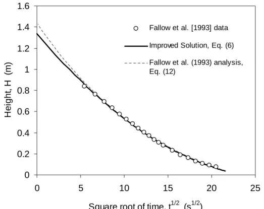
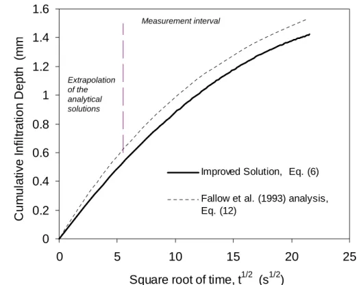
(5) Angulo-Jaramillo et al.. t 1/ 2 =. (H o − H ) a ⋅ 1/ 2 A  ∆θ φ m  2∆θ K fs H (t ) + b   . (12). The nonlinear least squares fit of Eq. (12) of the falling head data gave (Fallow et al.1993): Ho = 1.44 m, Kfs = 1.44 10-8 m/s, φm = 8.2 10-9 m2s-1 with α* = 1.76 m-1. They also pointed out that the fitting procedure is very sensitive to the initial guess value of Ho. Their sorptivity, So, and ponded sorptivity, SHo, Eq. (2), were 6.91 x 10-5 and 1.343 x 10-4 m s-1/2, respectively. Equation (6) was fitted on the data of Fallow et al. (1993) to estimate three parameters using the nonlinear fitting procedure of Elrick et al. (1995). Optimized parameters were Ho, Kfs, and So (Table 1); SHo, φm, and α* were calculated from Eqs. (2), (10), and (11), respectively. From the results in Table 1, the α and β parameters of Eq. (6) were calculated to be 1.070 10-4 m s-1/2 (Eq. (7)) and –1.907 10-6 m s-1 (Eq. (8)), respectively. Note that β is a negative value taking into account the falling head effect on infiltration flux. The negative second term in Eq. (6) is then representative of the reduction of the infiltration flux because the surface pressure head decreases. Table 1. Estimated hydraulic properties from the improved solution of the falling head experiment of Fallow et al. (1993).. Parameter Ho, m Kfs, m s-1 So, m s-1/2 SHo, m s-1/2 φm, m2 s-1 α*, m-1. Improved Solution Eq. (6) 1.339 9.79 10-9 5.54 10-5 1.070 10-4 5.27 10-9 1.859. Results of Fallow et al. (1993) 1.44 1.44 10-8 6.91 10-5 1.343 10-4 8.2 10-9 1.76. There is a small change in Ho estimated from Eq. (12), rather than the estimate from Eq. (6). The new initial pressure head from Eq. (6) is 7.0% smaller than that initially obtained by Fallow et al. (1993). The hydraulic conductivity of Fallow et al. (1993) is greater than the new value by 47.1%, while the sorptivity is superior to the new value by 24.7%. The increase on both sorptivity and hydraulic conductivity on Fallow et al.’s (1993) results from the fact that Eq. (6) has one more term than Eq. (1), the term β. However, Eq. (12) approximates the experimental data as well as Eq. (6) (Fig.1). From the results, Eq. (12) overestimates Ho, So, and Kfs, respectively, as compared to Eq. (6), agreeing with the results of Haverkamp et al. (1988). While the estimated parameters are used to predict the depth of water infiltrated (Fig. 2), it appears that the values of the depth infiltrated predicted using the result of Fallow et al. (1993) is higher than the improved equation. The.  Hydrology Days 2003. 20.

(6) Analysis Of Short-Time Single-Ring Infiltration. depth of water infiltrated is calculated as the volume infiltrated starting from Ho taking into account the surface area of infiltration. A consequence of the lower estimated Ho is a decrease in the calculated cumulative infiltration, IF = R(Ho-H), using the same H(t) data. The cumulative infiltration depth calculated for the time interval from t = 0 to the first measured H(t) value (Fig. 2) is an extrapolation of the infiltration equation. In the falling head problem, the pair (to, Ho) is an unknown. Unfortunately, in the case analyzed it was not possible to verify the total depth of water infiltrated into the soil. An independent measurement of the depth infiltrated would be necessary to validate the results. This type of measurement could be obtained using two methods. A destructive test consists of making a detailed analysis of the test site, for example by initial and final soil samples, to determine the variation in the total stored soil moisture content and thereby calculate the depth of water infiltrated corresponding to the final time of infiltration. This method was successfully used by Gérard-Marchant et al. (1997) in the characterization of a swelling soil under tests with variable and fixed pressures. In a non-destructive manner, the utilization of time domain reflectometry (TDR) techniques to measure either the soil water content or stored soil water would give an idea of the transitory regime of infiltration.. Height, H (m). 1.6 1.4. Fallow et al. [1993] data. 1.2. Improved Solution, Eq. (6) Fallow et al. (1993) analysis, Eq. (12). 1 0.8 0.6 0.4 0.2 0 0. 5. 10. 15 1/2. Square root of time, t. 20. 25. 1/2. (s ). Figure 1. Comparison between measured falling head as function of square root of time and the best fit of both, non-gravity result of Fallow et al. (1993) (dashed line) and for the improved solution (solid line)..  Hydrology Days 2003. 21.

(7) Angulo-Jaramillo et al.. 1.6 Cumulative Infiltration Depth (mm. Measurement interval. 1.4 1.2 Extrapolation of the analytical solutions. 1 0.8 0.6. Improved Solution, Eq. (6). 0.4. Fallow et al. (1993) analysis, Eq. (12). 0.2 0 0. 5. 10. 15. 20 1/2. Square root of time, t. 25. 1/2. (s ). Figure 2. Comparison between the cumulative infiltration data as a function of t1/2, calculated taken into account the estimated value of Ho. 6.. CONCLUSIONS Analysis of falling head infiltration tests over short time periods is an interesting alternative for hydrodynamic characterization of low permeability materials. In addition to not requiring sophisticated equipment, the time of the test is reduced as introduced by Elrick et al. (1995). As shown, not taking into account gravitational effects in the infiltration equation leads to an overestimation of hydrodynamic parameters estimated based on falling head infiltration tests, compared to those obtained from the general solution. This effect is accentuated by consideration of the ratio, R between the surface area of the supply reservoir and the water application surface area, leading to different estimates of the depth of water infiltrated. To make conclusions about the viability of one approach or another, it is recommended to perform an analysis at the test site of the volume of water infiltrated. This analysis can be made by measurement of the change in stored soil water in a one-dimensional infiltration profile. This permits verification of the amount of water effectively infiltrated into the soil. For example, GérardMarchant et al. (1997) used a destructive soil sampling method that gave a single value of the total depth of water infiltrated. Alternatively, another method could be the non-destructive continuous measurement of the change in soil water content using techniques such as TDR..  Hydrology Days 2003. 22.

(8) Analysis Of Short-Time Single-Ring Infiltration. References Elrick, D. E., G. W. Parkin, W. D. Reynolds, and D. J. Fallow, 1995: Analysis of early-time and steady state single-ring infiltration under falling head conditions. Water Resour. Res., 31, 1883-1893. Fallow, D. J., D. E. Elrick, W. D. Reynolds, N. Baumgartner, and G.W. Parkin, 1993: Field measurement of hydraulic conductivity in slowly permeable materials using early-time infiltration measurements in unsaturated media. In Hydraulic Conductivity and Waste Contaminant Transport in Soils, D. E. Daniel, and S. J. Trautwein, Eds. ASTM STP 1142, Philadelphia, PA. Gérard-Marchant, P., R. Angulo-Jaramillo, R. Haverkamp, M. Vauclin, P. Groenevelt, and D. E. Elrick, 1997: Estimating the hydraulic conductivity of slowly permeable and swelling materials from single-ring experiments. Water Resour. Res., 33, 1375-1382. Green, W. H., and G. A. Ampt, 1911: Studies on soil physics, 1. The flow of air and water through soils. J. Agric. Sci., 4, 1-24. Haverkamp, R., J.-Y. Parlange, J. L. Starr, G. Schmitz, and C. Fuentes, 1990: Infiltration under ponded conditions: 3. A predictive equation based on physical parameters. Soil Sci., 149, 292-300. Odell, B. P., P. H. Groenevelt, and D. E. Elrick, 1998: Rapid determination of hydraulic conductivity in clay liners by early-time analysis. Soil Sci. Soc. Am. J., 62, 56-62. Parlange, J.-Y., I. Lisle, R. D. Braddock, and R. E. Smith, 1982: The threeparameter infiltration equation. Soil Sci., 133, 337-341. Parlange, J.-Y., R. Haverkamp, C. W. Rose, and I. Phillips, 1988: Sorptivity and conductivity measurements. Soil Sci., 145, 385-388. Philip, J. R., 1957: The theory of infiltration, 1. The infiltration equation and its solution. Soil Sci., 83, 345-357. Reynolds, W. D., and D. E. Elrick, 1990: Ponded infiltration from a single ring. 1. Analysis of steady flow. Soil Sci. Soc. Am. J., 54, 1233-1241. White, I., and M. J. Sully, 1987: Macroscopic and microscopic capillary length and time scales from field saturation. Water Resour. Res., 23, 1514-1522..  Hydrology Days 2003. 23.

(9)

No results found