Master thesis in Structural Engineering
Characterisation of laminated glass for
structural applications
Authors: Shaheda Tahmina Akter
Mohammad Sadegh Khani Supervisor, LNU: Erik Serrano
Examiner, LNU: Hamid Movaffaghi Semester: Spring 2013, 15 credits Course code: 4BY05E
Abstract
Laminated glass (LG) consists of two or more glass layers bonded by an elasto-polymeric layer, the most commonly used being PVB (Polyvinyl Butyral). LG has improved safety properties compared with single layer glass because the interlayer prevents large sharp pieces from spreading when the glass is broken by impact. Even if one of the layers breaks, the other layer(s) still contribute in carrying the load. Through proper understanding of the interaction between the interlayer and the glass LG could be used in engineering as a load bearing material to a larger extent. This study aims at gaining a deeper knowledge of the behaviour of laminated glass by experimental investigations and by numerical model simulation. To pursue the proposed study, three point bending test with simple support conditions were performed for single layer glass and laminated glass units with three different types of interlayer materials. Corresponding finite element numerical models were created in the software ABAQUS to fit the model with experiment to obtain the bending stiffness and shear stiffness of the interlayer material. The PVB tested showed viscos-elastic material properties, whereas other two interlayer materials, Solutia DG 41 and Sentry Glass, showed linear elastic properties. PVB is the least stiff interlayer material among the three types. Solutia DG 41 and Sentry Glass have similar stiffness, about 13 to 15 times stiffer than the PVB. The behaviour of laminated glass lies in general between the two limits of a layered glass unit with no interaction and a monolithic unit of the same total thickness, depending on the stiffness of the interlayer material. Failure tests of the specimens were also carried out. The obtained strength of glass from four specimens is 80 MPa to 92 MPa with a variation of about 15%. The number of more performed experiments would have better outcome for strength of glass. The bending stiffness of the laminated glass as estimated with the numerical model fitted well with the experimental results with an error of about 2%. Hence the experimentally and numerically obtained results show a good correlation and are thought be possible to use in future larger scale modelling.
Acknowledgments
First of all, we would like to express our gratitude and cordial thanks to our supervisor Erik Serrano for his worth-while and constructive key-guidance to successfully complete this project in time. We are indeed happy to see his distinguished comments and notation that has helped us to upgrade the level and quality of this project.
We would like to give special thanks to Bertil Enquist for his experienced support, time and shared-thought to make our laboratory work successful. We also like to give a warm thanks to Jerry Eriksson of Glafo (Glass research institute) who arranged the materials for our experimental test. Also thanks to Kite Glass Ltd., UK for their help in supplying those materials to us. We would also like to thank our friends for their encouragement and supports.
Finally, we are grateful to our family and parents for their inspiration and patience to see our project completed.
Shaheda Tahmina Akter &
Contents
1. Introduction ...1
1.1 Background ...1
1.2 Purpose and aim ...2
1.3 Hypothesis and limitations ...2
1.4 Reliability, validity and objectivity ...3
1.5 Expected results ...3
2. Literature review ...4
2.1 The material glass ...4
2.2 Types of glass ...4
2.2.1 Float glass ...4
2.2.2 Annealed glass ...5
2.2.3 Laminated glass ...5
2.3 Mechanical Properties of glass ...6
2.4 Previous Research ...6
3. Theory ...8
3.1 Linear elasticity ...8
3.2 The finite element method... 10
3.2.1 The strong form... 10
3.2.2 Weak form ... 12
3.2.3 The finite element formulation ... 13
3.3 Mathematical equation for displacement of LG with PVB ... 15
4. Methodology ... 16
4.1 Sample selection and equipment for experiment ... 16
4.1.1 Test samples... 16
4.1.2 Equipment ... 17
4.1.3 Experimental set up ... 17
4.1.4 Analysis of experimental result ... 18
5. Results ... 21
5.1 Results for bending stiffness ... 21
5.1.1 Results for single layer glass ... 22
5.1.2 Results for LG with PVB interlayer ... 26
5.1.3 Results for LG with DG 41 Solutia interlayer ... 30
5.1.4 Results for LG with sentry glass interlayer ... 35
5.2 Result for Strength test ... 42
5.2.1 Result for strength test of single layer glass ... 42
5.2.2 Strength test result for LG with PVB interlayer ... 44
5.2.3 Strength test result for LG with DG 41 Solutia interlayer ... 46
5.2.4 Strength test result for LG with sentry glass interlayer ... 48
6. Analysis of results and discussion ... 51
6.1 Analysis of results on behaviour of laminated glass... 51
6.2 Analysis of results on strength of strength test ... 52
7. Conclusions ... 53
8. References ... 54 Appendix ... A-1
1. Introduction
Laminated glass is a type of building material which is used as a transparent material in construction of large buildings, especially in edifices with large facades. The lamination consists of two or more glass panes with a thin interlayer; Polyvinyl Butyral (PVB) is the most frequently used material. In an autoclave the interlayer bonds together with the glass panes at elevated temperature and pressure. PVB is an elastomeric polymer (Asik and Tazcan, 2005) that prevents the glass splinter from scattering in the case of breakage. Apart from this safety measure, thermal isolation, sound insulation, ultraviolet radiation absorption and moisture insensitivity (Foraboshi, 2007) makes the laminated glass popular in architectural glazing and also in automobile industry. Moreover, interlayer increases considerably the damping capacity of façade against loads and especially in case of dynamic loads (Aenlle, et al. 2011).
Despite its many advantages, the use of laminated glass as structural load carrying glass is still limited (Foraboshi, 2012) in the building sector. The combination of a brittle and hard material (glass) with a flexible and soft material (interlayer) makes the prediction of real behavior hard. Thus, through proper understanding of the interaction behavior of laminated glass it would be possible to introduce it to a larger extent as a load carrying material in the construction industry and in structural engineering.
1.1 Background
The use of glass as a load bearing, structural unit is being investigated within a co- European Wood Wisdom Net research project (LBTGC – Load Bearing Timber Glass Composites). As mentioned earlier some great advantages of laminated glass over single layer glass and monolithic glass have increased its uses significantly in contemporary building architecture. But compared with other structural materials like concrete, wood and steel, knowledge about structural behaviour and mechanical properties of laminated glass is not as well developed.
The modulus of elasticity (MOE) of glass is about 70 GPa whereas for PVB it is a few MPa only. The thickness of a typical PVB-layer varies from 0.38 mm to 1.52 mm (multiple of 0.38 mm), but typically 0.38 mm or 0.76 mm thickness is used. The great mismatches in material property and geometry make the mechanical and structural behaviour of laminated glass (LG) complicated. The modelling of LG with PVB is sophisticated because of the complex nonlinear behaviour (Ivanov, 2006) of PVB. Due to this complex manner LG is not very well modelled for structural use in previous research.
The behaviour of an LG unit when studying its stiffness and strength is considered to lie in between two limits. The lower limit corresponds to a layered glass unit with glass panes that are free to slide in relation to each other while the upper limit corresponds to a monolithic glass structure – a single pane glass unit with a thickness equal to that of the laminated glass. Some extensive efforts have been put on research on the issue, especially on mathematical and numerical engineering methods. However, these methods have not yet reached an adequate level of maturity (Foraboshi, 2012). Therefore, before applying laminated glass as a load bearing material in large scale, more knowledge on the interaction behaviour of different interlayer materials with glass (ordinary float or heat strengthened) is needed to know the mechanical properties and design strength of laminated glass.
In this study an experimental investigation and a numerical analysis by FE-modelling in ABAQUS will be carried out. Also some parametric study will be performed, to fit the FE-model to the experiments. The results from this study will be reported together with other studies within the above-mentioned co-European research project.
1.2 Purpose and aim
The purpose of this study is to increase knowledge of the interaction behaviour of glass sheets laminated with different interlayer materials for structural applications.
More specifically, the aim of this project is to characterise the interaction behaviour of different lamination foils bonded to glass, in terms of bending stiffness of laminated glass units, and to compare this behaviours with single layer annealed glass by experimental investigations and by finite element model simulations. By proper simulation the bending or shear stiffness obtained from ABAQUS modelling for lamination foils could be use in future larger scale investigations.
1.3 Hypothesis and limitations
1) Hypothesis: The test machine (MTS - Material testing services) and the proposed test set-up can be used to accurately measure load and deflection such that the test data sought can be recorded.
Limitations:
a) The machine can be equipped with various load cells ranging from ± 1 kN to ±100 kN. The assumed maximum load applied in the tests to be performed is 100 N – 500 N. Hence there may be some errors (1%) in measuring load and also deflection. The extent of these limitations is, however, judged to be of less importance.
b) Supporting the glass unit is also problematic (3-point simply supported case). Main problem that is foreseen relates to the precision of the test set-up (loading device and supports). If not accurately fitted, any misalignment between supports and loading device could lead to premature glass breakage during testing or very misleading load-displacement values due to e.g. twisting.
c) The experimental investigation is performed primarily for very short time load duration. In real life, the load duration for a structure is not as short as in the experiments. The behaviour of LG with different lamination foils could be different for lower magnitude long term loading as compared to short term loading (as in the experiments).
2) Hypothesis: The interlayer materials can be described as linear elastic materials by assigning e.g. shear modulus value (G) or modulus of elasticity (E) and Poisson’s ratio (ν) in ABAQUS.
Limitations:
a) PVB is a highly visco-elastic (Sobek et al. 2000 in Ivanov, 2006:6888) material. All polymer interlayers are visco-elastic (Annonymous, SentryGlas®).Thus elastic property is not accurately define the behaviour of visco-elastic property. But Ionoplast interlayer (Sentry Glass) is not as highly visco-elastic like PVB (Bennison, 2008).
b) PVB is a highly temperature dependent (Sobek et al. 2000 in Ivanov, 2006) material. Experiments only at room temperature are not enough to reach general conclusions about the behaviour of LG with PVB.
1.4 Reliability, validity and objectivity
The MTS 322 material test frame is appropriate for the bending tests. The methods (experiment and numerical simulation) are suitable enough to characterise the behaviour of different types of laminated glass and compare those with a single layer glass unit. In the experimental work, as small loads and deflection are concerned, the internal actuator of the testing machine could give misleading results due to any miss-alignment of the set-up. Thus, in addition to the internal actuator, two external LVDT (linear variable differential transformer) sensors were used to measure the displacement at two central points. This made the test procedure more reliable.
ABAQUS is a powerful tool for numerical analysis. A 2-D model was created in ABAQUS to gain more in-depth knowledge of the interaction behaviour of laminated glass and also to be able to differentiate the material behaviour of different foils used in the lamination. The ABAQUS model was verified by the experimental result. A comparison of the experimental results has been carried out by using mathematical relations derived by Asik and Tezcan (2005) for LG with PVB interlayer, which significantly validates the experimental results as well as numerical models.
Three point bending test at room temperature with simply supported laminated glass beam is not sufficient enough to give general conclusions on the structural behaviour of laminated glass for all kind of loading situations. The behaviour is of course also dependent on e.g. other modes of loading than pure shear (which is assumed in the tests) Also local phenomena at supports (other support conditions) and temperature could influence the results.
1.5 Expected results
1. To gain knowledge on behaviour of laminated glass for structural applications by experiment and also by numerical modelling.
2. To be able to differentiate the behaviour of lamination effect with PVB and other interlayer material in laminated glass unit.
3. To be able to do correct simulation of single layer glass and laminated glass units by using the finite element method (ABAQUS).
2. Literature review
This section firstly gives a brief description about glass, float glass, annealed glass, laminated glass, properties of glass and then a short review of previous research in this field for last decade.
2.1 The material glass
Glass is an inorganic product (Shand, 1958) which is formed by a process of cooling down into a rigid condition without crystallization. This means that glass is allied to liquid state materials.
Commercial glasses are mostly made of inorganic oxides of which silica is an important constituent. Only a limited number of oxides take part in forming glasses. Four primary operations take place in the glass manufacturing process. These are: batching, melting, fining and forming. The first three processes take place in almost all kinds of glass manufacturing, while the last one (forming and subsequent post processing) depends on the end product (Fröling, 2011).
2.2 Types of glass
Depending on the chemical composition of the glass, commercial glasses are subdivided into silica glass, soda-lime glass, lead -alkali silicate glass, borosilicate glass etc.
During the post processing state, glass products with some specific properties can be manufactured which allow its use extensively in the construction industry. Some of them are listed below:
1. Float glass 2. Annealed glass 3. Fully tempered glass
4. Toughened glass (Tempered glass) 5. Heat strengthen glass
6. Chemically strengthen glass 7. Laminated glass
Among these, float glass, annealed glass and laminated glass are described briefly as related to this study.
2.2.1 Float glass
Most flat glass or plate glass which is used as architectural glazing is soda-lime glass produced by the float glass process. This process was invented by Mr Alastair Pilkington of Pilkington glass in the 1950s (Anonymous, architectural glass). In this process molten glass is poured onto a bed of molten metal. Typically tin is used as molten metal for float glass, although lead or sometimes other low melting point alloys also used. The glass floats on that metal by which it achieves a smooth surface on both faces. The glass is then annealed by cooling in an oven called Lehr to relieve internal stresses.
2.2.2 Annealed glass
Annealing is a special process of slowly cooling glass, by which internal stresses are relieved from it .This is carried out in a temperature controlled kiln. Glass is annealed if it is heated above its transition point and then cooled very slowly. It is the first glass material to produce more advanced products through further treatment or processing. Float glass is annealed during the process of manufacturing .Annealed glass breaks into large shards.
2.2.3 Laminated glass
Laminated glass was invented in 1903 by a French chemist, Edouard Benedictus (Anonymous, laminated glass). He got inspired to invent this by a laboratory accident: A glass sheet that was coated with plastic cellulose nitrate did not break into sharp pieces when dropped. Gradually the process of lamination changed to today’s modern laminated glass. Nowadays, LG is typically made of two glass plates sandwiched by a thin plastic interlayer; mostly PVB (Polyvinyl Butyral) is used. PVB is a resin like material normally used for strong bonding. Apart from PVB also other materials are used, recent examples being e.g. Solutia DG 41 and Sentry Glass that were introduced in the laminated glass industry to meet the needs for high performance (Bennison, 2008) hurricane resistance glazing. DG is a resilient film (Anonymous, Saflex) produced from plasticized polyvinyl Butyral. Sentry Glass is an Ionoplast or ionic polymer (Blyberg, 2011) interlayer material. Both of these interlayer materials have higher stiffness property than PVB. Ionoplast comprises of primarily ethylene/ methacrylic acid copolymers containing small amounts of metal salt (Bennison, 2008), which has Young’s modulus of elasticity at least 100 MPa for temperature up to 50º C.
All of the above-mentioned interlayer materials have the same transparency as glass. The interlayer is placed in between two glass panes and the assembly is then placed in an autoclave with high pressure and temperature which makes the interlayer adhere to the glass. The interlayer allows the glass to be bonded together if the glass is shattered. The following Figure 2.1 describes the difference in breaking pattern of single layer glass and laminated glass.
(a) (b)
The strength of the interlayer prevents the glass from falling apart into large sharp pieces and therefore increases safety by reducing the risk of getting hurt by sharp shreds. Also, if one layer of glass breaks the other layer of laminate could carry some of the load.
2.3 Mechanical Properties of glass
The mechanical properties of glass depend on the crystalline solids (Shand, 1958) of it. It has elastic properties which allow it to regain its original shape after reloading. It has no plastic properties like e.g. metals and consequently no yield point. Fracture occurs before any permanent deformation takes place. Failure always happens in tension because it has high compressive strength. For stress calculation, glass can be considered a homogeneous and isotropic material.
2.4 Previous Research
Research has been carried out on behaviour, strength, analytical and numerical modelling of laminated glass with PVB over the last few decades. Glass has a modulus of elasticity (MOE) several thousand times larger than the MOE of the weakest interlayer material, PVB. This great mismatch makes the behaviour complex as well as analysis and modelling of laminated glass. According to Asik (2005) first research on LG beam was done by Hooper in 1973.After that and until 1985 no major research was carried out in this field. Some research has been conducted after this on behaviour, strength, analytical and numerical modelling of laminated glass with PVB but still the knowledge required to use laminated glass as a load bearing element in every-day construction, is not sufficient.
Norville et al. (1998) developed a theoretical model of laminated glass beams with uniformly distributed load. They derived a mathematical model by considering factors like interlayer thickness, composition of interlayer and temperature, which affect the behaviour of laminated glass. They assumed that the interlayer (PVB) performs no other function but maintaining the spacing between the glasses plies and transfers a fraction of the horizontal shear force between the glass plies. The PVB increases the section modulus of the laminated glass and therefore reduces the magnitude of flexural stresses in the outer glass fibres. They mentioned a shear transfer coefficient on which the amount of horizontal shear force transfer by the interlayer to the glass plies depends. The value of this parameter varies from 0 to 1 and needs to be calculated from experimental data. When this parameter is zero laminated glass acts like a layered beam with symmetrical stress distribution on both glass plies. When the parameter is one it behaves like a monolithic glass beam. By this, an expression for effective section modulus was derived. They verified their mathematical model by the experiments done by Behr et al. in 1993. One important conclusion from their research was that flexural strength of laminated glass decreases with increase in temperature.
Duser et al. (1998) had done a three dimensional finite element model for stress development with statistical model for glass fracture. They used the approach by Bennison et al. (1998) to analyse biaxial bending of disks. They used non-linear analyses, defining PVB as a visco-elastic material. They found that stress development is influenced by loading rate and temperature.
Asik and Tezcan (2005) presented a mathematical model of laminated glass beams considering large deflection. The model is able to predict the behaviour of monolithic, layered and laminated glass beams. They derived the mathematical model by using the principles of minimum potential energy and applying variational principles. They obtained three coupled nonlinear differential equations to explain the behaviour of laminated glass beams. They verified the model by using data obtained from simply supported three point bending test and did numerical modelling (beam with fixed supports and a concentrated load in the centre). They reported an error of the mathematical model results of about 24% as compared to the experimental results. They concluded that simply supported LG beam shows linear behaviour even for large deflection but fixed supported LG beams show non-linear behaviour due to the effect of membrane stresses.
Ivanov (2006) developed an analytical model for laminated glass beam consisting of differential equations for bending curvature and shear interaction for the PVB interlayer. It is claimed in that research paper that the derived equation for deflection is similar to the equation derived by Asik and Tezcan (2005). The theory is verified by a mathematical model in MATLAB. A finite element model was constructed for a simply supported beam with transverse loading. The laminated glass was modelled by using plane multilayered beams with linear elastic material for glass and PVB. The research showed that the bending stress in the glass layers is determinant for the load carrying capacity of laminated glass but shear in the PVB plays an important role in the interaction. The mathematical model was utilized in a lightweight structure to optimize layer thickness and it showed that laminated glass could be better than monolithic glass. The model is confined to small strain and displacements.
As per authors knowledge no similar research has been carried out on laminated glass with interlayer of Solutia DG 41 and Sentry Glass. It is very important to know the behaviour of the LG with these two interlayers also for structural uses purposes, as they have higher rigidity than PVB.
3. Theory
The purpose of this section is to describe some necessary theory which is related to the experimental and numerical approaches used in the project. In this part the constitutive relation between stress and strain for linear elasticity, the final equation derived by Asik and Tezcan in 2005 and the fundamentals of the finite element method are presented.
3.1 Linear elasticity
A material is called elastic material if it retakes its original state after removing applied loads. The elasticity of a material can be described by one-to-one stress-strain relation. If the relation between stress and strain remains linear the material is called linear elastic. Often the assumption of small strain is also included in linear elasticity.
For a one dimensional case, linear elasticity is expressed by Hooke’s law, which states that stress is proportional to strain,
E (3.1)
The ratio of stress to strain thus remains constant and the ratio is represented by the modulus of elasticity (MOE) also known as Young’s modulus, here denoted by E. Figure 3.1 describes linear elasticity below.
Figure 3.1 Hooke’s law
The one-dimensional Hooke´s law can be expanded to two and three-dimensional cases also, and instead of one single equation expressing the relation between stress and strain, a matrix relation (a number of linear equations) is introduced instead. For the general three-dimensional case this is often expressed as
D (3.2)
66 62 61 26 22 21 16 12 11 ... ... ... ... ... ... ... D D D D D D D D D D ; yz xz xy zz yy xx ε (3.3)
Where, D is the constitutive matrix.
Figure 3.2 Stress components of a 3-D element
For isotropic materials, the D-matrix is independent of the (has the same value in every) coordinate system and only two independent material parameters exist. Often the D-matrix is expressed in terms of the Young’s modulus and the Poisson’s ratio.
) 2 1 ( 2 1 0 0 0 0 0 0 ) 2 1 ( 2 1 0 0 0 0 0 0 ) 2 1 ( 2 1 0 0 0 0 0 0 1 0 0 0 1 0 0 0 1 ) 2 1 )( 1 ( v v v v v v v v v v v v v v E D (3.4)
The shear modulus, G, is then given by ) 1 ( 2 v E G (3.5)
Where, is the Poisson’s ratio.
3.2 The finite element method
The finite element method is a numerical way to solve arbitrary differential equations, in general in an approximate manner. It can be applied to various physical phenomena. By this means any arbitrary area is subdivided into small elements, so-called finite elements and a simplified approximation of the unknown quantity is made over each small element. Having determined the behaviour of all small elements i.e. knowing the element wise response, these are then put together by some specific rules to obtain the solution for the whole region. In the following section the FE formulation of three-dimensional / two-dimensional elasticity is described.
3.2.1 The strong form
For a three dimensional body in x, y and z plane
z y x t t t t (3.6)
Where, t is a traction vector acting on the boundary surface S and b is the body force (N/m3) in the region V.
Figure 3.3 Three- dimensional body with thickness t showing traction vector and body force
Equilibrium of the body requires,
S V
dV
ds b 0
t , (3.7)
S V x xdS b dV t 0
S V x T xndS bdV 0 s (3.8)
S V y ydS b dV t 0
S V y T yndS b dV 0 s (3.9)
S V z zdS b dV t 0
S V z T zndS bdV 0 s (3.10)Where it was used that the traction vector, t, can be written in terms of the symmetric stress tensor S, by the relation
z y x z y x z y x zz zy zx yz yy yx xz xy xx T n n n n n n s s s n S n S t (3.11)By Gauss divergence theorem, expressions 3.8-3.10 can then be expressed more explicitly by divS +b=0
Furthermore the following differential operator is used.
y x z z x y z y x 0 0 0 0 0 0 0 0 0 ~T (3.12)
And the stress vector can be written as:
yz xz xy zz yy xx σ (3.13)
For plane stress state the differential operator and stress vector become:
x y y x T 0 0 ~ (3.14) xy yy xx σ (3.15)
The equilibrium equations (for three or two dimensional cases) can be written in the compact matrix form as:
0 b σ
T
~ (3.16)
t=Sn=h on Lh natural boundary condition (load)
u=g on Lg essential boundary condition (displacement)
The kinematic equation relates the strain vector to the displacement vector by the use of differential operator as:
u
ε~ (3.17)
Whereas the relation between stress and strain was established in section 3.1
3.2.2 Weak form
In order to obtain the weak form according to the Galerkin method, equilibrium equation (3.16) is first integrated and multiplied by an arbitrary vector v, given by:
z y x v v v v (3.18)
The process yields the following equations for the 3-dimensional case,
V V Z Z Zz Zy Zx Z V V y y yz yy yx y V V x x xz xy xx x dV b v dV z y x v dV b v dV z y x v dV b v dV z y x v 0 ) ( 0 ) ( 0 ) ( (3.19)By using Green Gauss theorem and after some manipulation the weak form is finally obtained
V S V v σdV v t dS v bdV T T T ~ (3.20)u = g on Sg essential boundary condition For two dimensional cases this can be written as:
A T L T T A v σ dA v tdL v b dA ~ (3.21)Where, t = Sn = h on Lh natural boundary condition (loads)
3.2.3 The finite element formulation
The physical problem of the considered entire region is expressed in terms of the strong and weak formulations of three-dimensional elasticity. The FE method approximates the unknown element-wise and carries out the same approximation over the whole region to get the solution. The finite elements are connected with each other by nodes and the unknown parameters (displacements in elasticity problems) are continuous between elements connected to a certain node.
The approximation for displacement vector u at any point (x, y z) within an element can be written as
(3.22)
The strain vector at any point,
e e e e a B a N ~u ~ yz xz xy zz yy xx (3.23) e e zn yn xn z y x z y x e n e e e n e e e n e e z y x a N u u u u u u u u u N N N N N N N N N u u u ., 0 0 ... 0 0 0 0 0 0 ... 0 0 0 0 0 0 ... 0 0 0 0 2 2 2 1 1 1 2 1 2 1 2 1 u
Where, y z x z x y z y x 0 0 0 0 0 0 0 0 0 ~ e e N B e n e e e n e e e n e e N N N N N N N N N 0 0 ... 0 0 0 0 0 0 ... 0 0 0 0 0 0 ... 0 0 0 0 2 1 2 1 2 1 (3.24)
The next step is to choose the arbitrary weight function by the Galerkin method, which means that the same type of functions are used for the weight functions as for the approximation function. The approximation for the weight vector v by the Galerkin method is thus
Nc
v and ~vBc (3.25)
Where, weight function v and c matrix are arbitrary.
Insertion of these expressions in the weak form yields the FE formulation,
0
V S V dV dS dV N t N b σ B cT T T T (3.26)As the c-matrix is arbitrary, this can be written as
V S V dV dS dV N t N b σ BT T T (3.27)This equation corresponds to the relation between the stiffness matrixK , displacement e vector aeand the element load vectorf :e
e e e f a K (3.28)
On the basis of this form, finite element software evaluates by numerical integration the element stiffness matrices to calculate the global stiffness matrix and global load vector and finally obtain a solution for the displacement vector. Following this, element displacements are extracted, from which stresses and strains are determined at the so-called integration points of the elements by the following relation,
DBa Dε
3.3 Mathematical equation for displacement of LG with PVB
As mentioned in chapter 2 , for validity of this research project the results obtained from experiments and FE modelling are compared with a mathematical equation derived (for displacement) by Asik and Tezcan in 2005 (page: 1747):
) ( 1 cosh sinh 1 2 1 cosh ) ( cosh ) 4 ( 24 ) 3 )( 2 ( 6 ) 2 ( 2 1 ) ( 6 4 1 3 4 2 2 3 2 2 4 2 1 2 1 N x Gb t h x L x p L L x q x L x q x L x P qL Lx x q A EA A A h x w t t (3.30) Where, I h A A A A Et Gb t2 2 1 2 1 2 and I h Et Gb t x L x p cosh sinh 1 2 4 L x P L L x q x q x P qL q N cosh sinh 2 cosh ) ( cosh 2 ) 2 ( 3 4 2 2 2 4 1
A1 and A2 = cross-sectional area of top and bottom glass plies ht = total thickness of laminated glass unit
b = width of beam
t = thickness of interlayer material L = length of beam
q = uniform distributed load on beam P = concentrated load on the centre of beam x = co-ordinate along x axis
4. Methodology
Methodology is the process, by which the project is carried out. The project is carried out mainly by two methods:
a) By experiments in laboratory.
b) By numerical analysis using FE modelling.
Firstly the test set up in laboratory and then details of FE modelling are described below.
4.1 Sample selection and equipment for experiment
4.1.1 Test samples
Four types of specimens, shown in Figure 3.4, were selected for experiments. All specimens were supplied by Kite Glass Ltd., UK, through Glafo (Glass research institute).
1) 10 specimens of 6 mm thick single annealed glass. Length 500mm and width 75mm. 2) 10 specimens of 12.76 mm thick laminated glass with PVB material interlayer. Length
500mm and width 75mm.
3) 10 specimens of 12.76 mm thick laminated glass with Solutia DG 41interlayer. Length 500mm and width 75mm.
4) 10 specimens of 12.89 mm thick laminated glass with sentry glass interlayer. Length 500mm and width 75mm.
4.1.2 Equipment
The MTS 322 material test frame at the laboratory of the Department of Building and Energy Technology of Linnaeus University was used to perform the proposed three point bending test. This machine is used to measure central deflection and the corresponding applied load for a simply supported beam in three point bending.
This servo-hydraulic model of the MTS 322 test frame has a force capacity up to100kN. It has different load cells: 100kN, 10kN and 1kNwhich help to set up the desired load. The 1kN load cell is used to perform the test for this project. Although the MTS is equipped with a high accuracy internal actuator to measure displacement, two extra external LVDT (linear variable differential transformer) were used to measure the central displacement in order to capture possible twist during the test.
Figure 4.2 MTS 322 material test frame
Above Figure 4.2 shows the machine MTS 322.
4.1.3 Experimental set up
A three point flexural set up has been chosen to perform the experiment for this project. A safe load level was calculated prior testing such that measuring maximum deflection could be done without the glass would forming any cracks.
Two metal roller supports of 60 mm diameter placed on two metal plates were used to support the glass beam along its entire width.
Similarly for applying load, a device with 15 mm diameter was fitted into the grips of the machine. As mentioned earlier two external LVDT sensors were fitted under the test specimen to measure deflection at two different central position .One LVDT sensor was placed on each side of the specimen. Details of the test set-up is shown in Figure 4.3
Figure 4.3 Test set up
A displacement of 1mm was applied in central part of beam by the loading device. The load range selected was up to 500 N. The considered length of the free span for single layer glass and LG with PVB was 300 mm, for LG with DG Solutia it was 350 mm and for LG with sentry glass it was 400 mm. 5 samples of each type of specimen were selected for experiments.
The proposed displacement is applied at the rate of 0.5 mm per min to all types of specimen. At every 0.2 sec the displacement and corresponding load is sampled and recorded.
One laminated glass samples with PVB interlayer was exposed to a constant 1 mm displacement for a two hour period to investigate any possible change in load with time (visco-elastic behaviour, creep/relaxation).
4.1.4 Analysis of experimental result
The deflection recorded during experiments for LG with PVB foils was compared with the theoretical expressions derived for deflection by Asik and Tezcan (2005). The results of the experiments were analysed to get the initial bending stiffness of the material, which was then compared with the results from the ABAQUS model and used to understand the structural behaviour of the laminated glass for different interlayer materials.
4.2 Numerical model
The numerical modelling of laminated glass by finite element method is complex; mainly because of the very thin interlayer in comparison with other dimension and because of the large difference in modulus of elasticity of glass ply and interlayer material, specially for PVB. The numerical result of LG with PVB exhibits high sensitivity to the glass ply-to-interlayer moduli ratio Eg / GPVB (Bažant and Beghini 2004 in Foraboschi, 2007:1291).
Due to the very thin interlayer, the necessary degree of discretization in the thickness direction will require high degree of discretization in the other directions (Ivanov, 2006). Therefore more computational work would be involved. As the aim of this numerical model is to fit with experiment hence more time consuming and computationally expensive 3-D model is not found suitable by the authors for this parametric study .Therefore a 2-D model with plane stress state in ABAQUS is used which can still accurately represent the behaviour of LG. Symmetry in x-direction is used to reduce the model size in ABAQUS.
To model the roller support and the load device two 2-D analytical rigid parts were created according to the dimension of the laboratory test set-up. The parts are then assembled and interactions between the parts are created. The friction coefficient between glass and metal is set to 0.6. The ABAQUS models for the single layer glass and different types of laminated glass are shown in Figure 4.4, 4.5 and 4.6.
A comparison study for displacement and stress carried out for different element types and mesh sizes is presented in chapter 5.1. Finally four node bi-linear quadrilateral solid elements (with incompatible modes that improve their bending behaviour) of size 0.25 mm were adopted to best fit the model with experiment and to get Young´s modulus and Poisson’s ratio for glass and different interlayer materials. Figure 4.7 presents the adopted mesh for a laminated glass.
Figure 4.4 Numerical models for single layer glass
Figure 4.6 Numerical model of LG with sentry glass
There was some variation of nominal size and actual size measured for the different specimens in the laboratory. In the above figures nominal sizes are shown whereas the models created in ABAQUS included the average of actual measured sizes of the specimens, see Chapter 5.
5. Results
The main aim of this project was to gain knowledge about and to characterise the behaviour of laminated glass in terms of bending stiffness, the corresponding result is presented in the first part of this chapter. In addition, the strength of different types of LG was also tested which is presented in the second part.
5.1 Results for bending stiffness
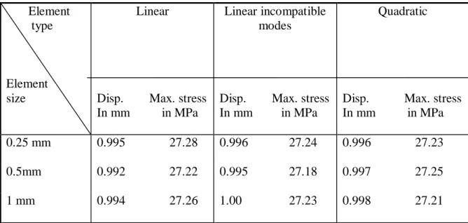
The results from experiments are presented here by considering the mean of measured displacements by two external LVDT. Curves are adjusted and set to start from 0 for both displacement and load. To get the initial stiffness of the specimens a 10 N to 100 N load range and corresponding displacements are used. Data points were evaluated by a linear regression method to get the slope corresponding to the initial stiffness. Then finally, the average of those slopes was used to obtain the modulus of elasticity for a specific specimen type. As mentioned in 4.2 the actual sizes of glass and different LG were found to be slightly different than the nominal sizes. The average of those actual sizes was considered in the calculations to obtain the E-modulus for the test specimens from the experimental tests and also in the ABAQUS model. In the FE model 160 N loads were applied for single layer glass whereas 500 N loads were applied for all types of LG to calculate the bending stiffness. Table 5.1 and 5.2 present the comparison study of displacement and stress of single layer glass and LG with PVB from FE model for different element types and sizes. The variation in stress is very small. As the aim was to fit the model with slope for initial stiffness obtained from experiments, it was found that linear element with incompatible modes for mesh sizes of 0.25 mm suits best.
Table 5.1 Comparison of displacement and stress for different element type and mesh size for single layer glass
Element type
Element size
Linear
Disp. Max. stress In mm in MPa
Linear incompatible modes
Disp. Max. stress In mm in MPa
Quadratic
Disp. Max. stress In mm in MPa
0.25 mm 0.995 27.28 0.996 27.24 0.996 27.23
0.5mm 0.992 27.22 0.995 27.18 0.997 27.25
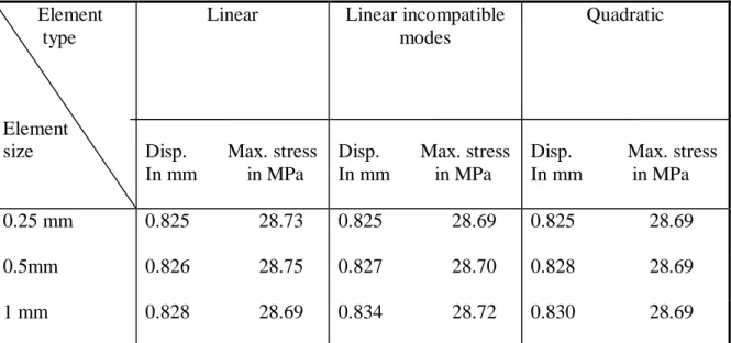
Table 5.2 comparison of displacement and stress for different element type and mesh size for laminated glass with PVB
Element type
Element size
Linear
Disp. Max. stress In mm in MPa
Linear incompatible modes
Disp. Max. stress In mm in MPa
Quadratic
Disp. Max. stress In mm in MPa
0.25 mm 0.825 28.73 0.825 28.69 0.825 28.69
0.5mm 0.826 28.75 0.827 28.70 0.828 28.69
1 mm 0.828 28.69 0.834 28.72 0.830 28.69
5.1.1 Results for single layer glass
The length of the free span for single layer glass was 300 mm. A 1 mm displacement was applied at the rate of 0.5mm per min. In Table 5.3 actual measured size of the single layer glass specimens is presented. Calculated average slope (initial stiffness) of the lines for load versus deflection curves of 5 samples is 158.7, which is given also in Table 5.3.The corresponding plots are presented in Figure 5.2.
Table 5.3 Modulus of elasticity calculated from Experimental data for single layer glass sample Effective Length in mm Width in mm Depth in mm Second moment of inertia in mm4 Slope of line (initial part, N/mm) E-modulus in MPa S_1 300 75.69 5.85 1262.8 157.9 70350 S_2 300 75.61 5.85 1261.4 157.6 70250 S_3 300 75.44 5.89 1284.6 159.4 69790 S_4 300 75.74 5.84 1257.1 159.3 71260 S_5 300 75.54 5.90 1292.9 159.5 69390 Average 75.60 5.86 1271.8 158.7 70210
The modulus of elasticity of glass, evaluated from experimental data is 70.2 GPa. By using this value in the ABAQUS model with Poisson’s ratio of 0.23, the model fitted with experiment with an error of 1.19 %. The slope of the load-displacement curve from ABAQUS is 160.6 N/mm. Table 5.4 presented below shows a comparison of the central deflection and the maximum principal stress at three load levels for the experiments (evaluated using simple beam theory) and for the numerical model.
Table 5.4 Comparison of result for single layer glass from experiment and numerical model
Load in Central deflection in mm Maximum principal stress ABAQUS Result N
Exp. N.Mod Error(%) Exp. N.Mod Error(%) E-Mod. in MPa Poiss. ratio 50 0.315 0.314 - 0.317 8.62 8.53 -1.04
100 0.630 0.623 - 1.07 17.25 17.03 -1.28 70200 0.23
150 0.945 0.934 - 1.16 25.87 25.54 -1.28
The following Figure 5.1 represents the plot for load versus displacement for full applied load range of single layer glass. It shows that the tests gave very consistent data, with similar slopes of all curves line.
Figure 5.2 Initial (stiffness) slopes of single layer glass
Figure 5.3 Stress S11 along mid section
In above Figure 5.3 the stress S11 from the FE model is shown along the mid-section of the single layer glass. The maximum tensile stress is 27.24 MPa on the bottom face and the maximum compressive stress is – 30.8 MPa on the top face for a 160 N load. The neutral axis
is located at 3.05 mm from the bottom face, thus being slightly shifted up from mid depth (2.92 mm) because of high compressive stress concentrations at the loading device on the upper face of the glass beam. The following Figure 5.4 presents stress distribution along a cross section at 75 mm from support. The difference of tensile and compressive stress is very small at that section in comparison to the mid-section.
Figure 5.4 Stress S11 along section 75 mm from support for single layer glass
5.1.2 Results for LG with PVB interlayer
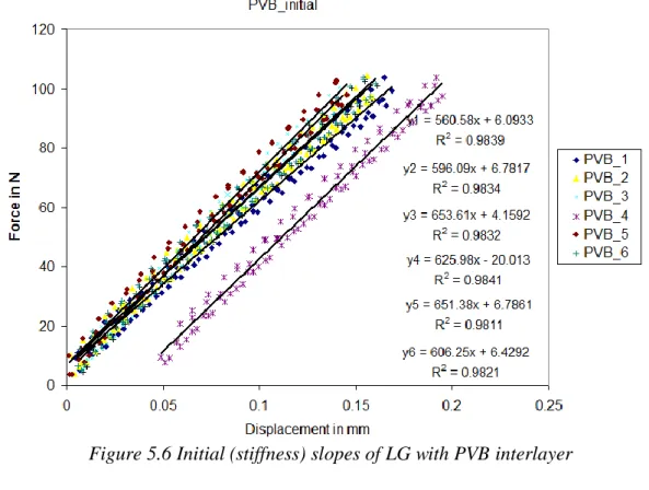
The centre to centre distance of the supports for LG with PVB interlayer was also 300 mm. 1 mm displacement was applied at the same rate of 0.5 mm per minute. The load limit was set to 500 N. In total 6 samples were tested instead of five due to some changing behaviour of this type of LG as compared to single layer glass. The measured actual dimensions of LG with PVB are presented in Table 5.5. Load versus deflection curves are shown in Figure 5.6 for full applied load range. It is clear from that graph that LG with PVB shows some non-linear behaviour that could be due to material nonnon-linearity.
The calculated average slope (initial stiffness) of the load versus displacement curves of 6 samples is 615.6, which is also presented in Table 5.5. The previously calculated modulus of elasticity and Poisson’s ratio for glass (Eg =70200 MPa, = 0.23) were used in the ABAQUS
model for LG with PVB. To match the calculated average initial stiffness slope obtained from experiment a parametric study was done by changing the E-modulus and Poisson’s ratio of the PVB with different types of elements and element sizes (reported in Table 5.2). The slope of the force-displacement curve finally obtained from the ABAQUS model is 606.1 N/mm, an error of -1.55 % as compared with the experiments.
Table 5.5 Initial stiffness values with measured original size of LG with PVB interlayer sample Effective Length in mm Width in mm Depth in mm Second moment of inertia in mm4 Slope of line (initial stiffness) Effective modulus of elasticity in MPa PVB_1 300 75.87 12.33 11851.6 560.6 26605 PVB_2 300 74.70 12.49 12129.0 596.1 27645 PVB_3 300 74.59 12.50 12140.3 653.6 30280 PVB_4 300 75.47 12.59 12550.8 626.0 28060 PVB_5 300 73.50 12.47 11877.0 651.4 30850 PVB_6 300 75.26 12.51 12278.8 606.2 27770 Average 74.89 12.48 12130.7 615.6 28540
A comparison of central displacement obtained from experiment and numerical model of LG with PVB is presented in the following Table 5.6 for some load levels. Also the calculated displacement by the theory derived by Asik and Tezcan in 2005 is presented here to compare with result obtained by experiments and FE model. Errornm and Errorth.m represent error of
Table 5.6 Comparison of result for LG with PVB interlayer from experiment and numerical model
Load in Central deflection in mm Properties of PVB from ABAQUS
N Exp. N. Model Theor, Model Errornm. Errorth.m E-mod. Poisson’s
(%) (%) In MPa ratio 100 0.162 0.165 0.162 1.85 0
200 0.325 0.332 0.324 2.15 - 0.31 9 0.42
300 0.487 0.496 0.486 1.85 - 0.21
400 0.650 0.661 0.648 1.69 - 0.31
Figure 5.5 Load versus central deflection for LG with PVB with full applied load range
Load versus displacement plot for initial stiffness slopes are shown in Figure 5.6 below. PVB_1 showed the least slope 560.58, whereas the maximum slope is 653. 61. The important noticeable difference in behaviour for LG with PVB was a load variation (the wavy pattern in the curves) as compared to the tests with single layer glass. The load variation was about10N, which makes a big difference in the estimation of the initial stiffness if single data points are evaluated. However, the chosen method of using linear regression over a larger interval is thought to be very sensitive to the variation. The variation might be due to either the interlayer material behaviour or due to some stick-slip behaviour of the test set up.
Figure 5.6 Initial (stiffness) slopes of LG with PVB interlayer
One sample of LG with PVB was tested to see time if any dependencies of the PVB interlayer with time could be recorded. A displacement of 1mm was applied and held for two hours and the corresponding load was recorded. The test result in terms of force versus time is plotted in Figure 5.7. It is clearly seen from that plot that there is a large difference in load within the first 500 sec, after this the change takes place with very slow rate.
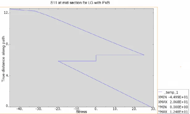
Following Figures 5.8, 5.9 and 5.10 present stress (S11) distributions along depth for laminated glass with PVB interlayer obtained from the FE models. It is seen from Figure 5.8 that maximum tensile stress along bottom edge is 28.68 MPa whereas maximum compressive stress along top edge is - 44.99 MPa. This high compressive stress concentration is around the loading device which is clear from the following figures.
Figure 5.8 Stress S11 at mid section for LG with PVB
Figure 5.10 Stress (S11) concentration for LG with PVB
The Table 5.7 presents the maximum tensile and compressive stress along mid-section for both glass layers of LG with PVB, obtained from FE model. Y coordinate is set to zero at the bottom face of the beam. For bottom glass plies the maximum tensile stress is 28.68 MPa, while for top glass plies it is 25.12 MPa for 500 N load. The behaviour of LG with PVB lies in between two limits (slightly avobe the lower limit i.e. layered glass). In the interlayer there are some shear transfer which is noticable from above three figures.
Table 5.7 Position of neutral axis and magnitude of maximum tensile and compressive stress for LG with PVB
Distance from bottom edge in mm Maximum tensile and compressive stress in Mpa
0 28.68
5.86 - 19.97
6.62 25.12
12.48 -44.99
5.1.3 Results for LG with DG 41 Solutia interlayer
The length of the free span for LG with Solutia DG 41 was set up to 350 mm. A displacement of 1 mm was applied at the same rate of 0.5mm per min with load limit of 500 N. This type of LG is stiffer than expected and had only a 0.67 mm average central displacement for a 500 N load. Hence the length was later increased to 400 mm for the remaining four samples. Moreover the first, short span sample, showed a clear nonlinear behaviour with increasing stiffness at higher load levels (Figure 5.11). This might be due to some unexpected behaviour of the test set-up. Therefore in calculation of bending stiffness for LG with Solutia DG 41, this sample result was not considered. Calculated average slope (initial stiffness) for this type
of LG is 558.2 for the other four samples. One sample has a somewhat different stiffness, while all other three have almost the same stiffness. The plots are shown in Figure 5.12. To fit this slope in the numerical model, MOE was found to be 120 MPa with Poisson’s ratio of 0.48.The slope of the force-displacement curve is 565.0 from ABAQUS, an error of 1.22% as compared with the experiments. Actual measured sizes of LG with DG 41 Solutia and initial stiffness values are presented in Table 5.8 below.
Table 5.8 Initial stiffness values with measured original size of LG with Solutia DG 41 interlayer sample Effective Length in mm Width in mm Depth in mm Second moment of inertia in mm4 Slope of line(initial part) Effective modulus of elasticity for LG unit in MPa DG_2 400 75.45 12.47 12269.7 539.1 58950 DG_3 400 75.47 12.59 12550.8 563.9 59900 DG_4 400 74.48 12.70 12713.6 565.4 59290 DG_5 400 75.37 12.47 12179.1 564.6 61810 Average 75.19 12.56 12408.9 558.2 59990
A comparison of central displacements obtained from experiments and numerical model of LG with Solutia DG 41 is presented in the Table 5.9 for some load points.
Table 5.9 Comparison of central deflection for LG with DG 41 Solutia interlayer
Load in N Central deflection in mm Properties of DG 41 Solutia
Exp. N. Model Error(%) E-modulus in Mpa Poisson’s ratio 100 0.179 0.178 - 0.726
200 0.358 0.355 - 0.837 120 0.48
300 0.537 0.532 - 1.04
Figure 5.11 Force versus central displacement for LG with Solutia DG 41 interlayer
Load versus displacement plots for full applied load range in the experiments are shown in Figure 5.11 above. The load variation (waviness of the curves) is less than LG with PVB. It is noticeable also from plots of Figure 5.11 that only one sample has some different stiffness, while the other three have almost the same stiffness (except the discarded DG_1).
Figure 5.12 Initial (stiffness) slopes of LG with Solutia DG 41
The plots shown in Figure 5.13, 5.14 and 5.15 are from the results of the ABAQUS model for LG with Solutia DG 41. Table 5.10 shows maximum tensile and compressive stresses for both
glass plies in LG unit obtained from the numerical model. It is found that maximum tensile stress at bottom face is 27.7 MPa, while the maximum compressive stress is – 41.2 MPa on top face of LG. This large difference in tensile and compressive stress is due to the loading device (like previous cases). Figure 5.14 presents stress (S11) distribution along section 125 mm from support, which shows that the difference between tensile stress (15.4 MPa) in bottom face and compresive stress (- 15.7 MPa) in top face of LG unit is very small in camparison of that along middle section. By analysing these figures and Table 5.10 of stress distribution it can be concluded that here the LG unit behaves more similar to a monolithic unit.
Figure 5.13 Stress S11 along mid-section for LG with DG
Table 5.10 Maximum tensile and compressive stresses along depth for LG with DG 41 Distance from bottom face in mm Maximum tensile and compressive
stresses in MPa
0 27.72
5.90 - 5.55
6.66 7.76
Figure 5.14 Stress S11 along section 125 mm from support for LG with DG
5.1.4 Results for LG with sentry glass interlayer
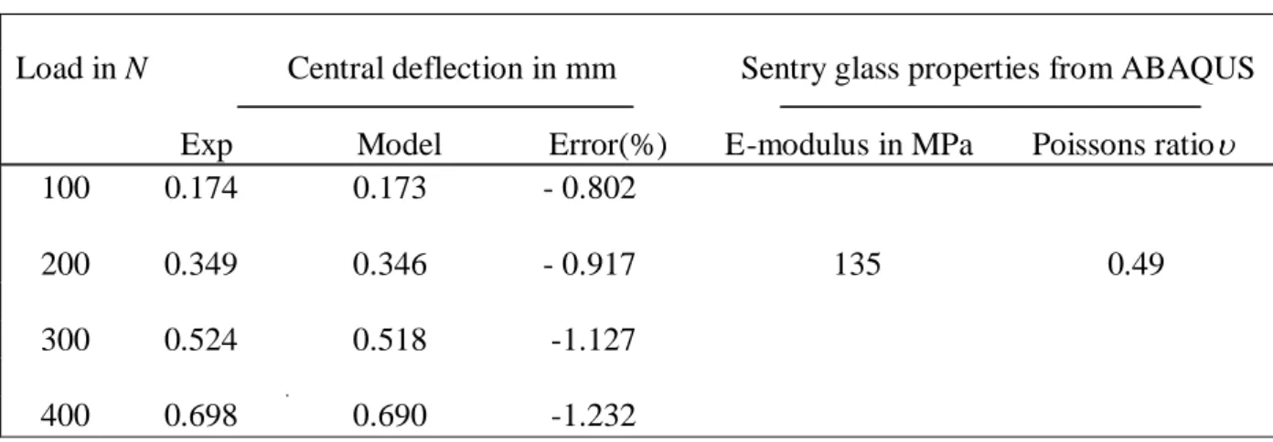
The centre to centre distance of support for LG with sentry glass was 400 mm. The applied displacement rate was 0.5 mm per min, while the load limit was set as maximum 500 N. Maximum central displacement of 0.833 mm was measured at a 500 N load. Calculated average slope (initial stiffness) of trend line of load versus deflection curve for 5 samples is 572.9, which is presented together along with actual measured width and depth of the different samples in the following Table 5.11. To fit with this slope, an ABAQUS model was created with an interlayer thickness of 0.89 mm (mentioned in chapter 4.2) with this average width and thickness of the LG unit. After fitting, the modulus of elasticity for sentry glass obtained from the ABAQUS model is 135 MPa, with a Poisson’s ratio of 0.49.The obtained slope from ABAQUS is 580.4 with an error of 1.3 %.
Table 5.11 Initial stiffness values with measured original size of LG with sentry glass interlayer sample Effective Length in mm Width in mm Depth in mm Second moment of inertia in mm4 Slope of line (initial stiffness) Effective modulus of elasticity of LG unit in MPa SG_1 400 75.70 12.78 12993.7 584.2 59950 SG_2 400 73.3 12.69 12482.7 557.0 59500 SG_3 400 75.09 12.79 13092.2 574.9 58550 SG_4 400 75.01 12.70 12804.1 575.2 59900 SG_5 400 74.48 12.76 12894.7 573.2 59270 Average 74.51 12.74 12853.5 572.9 59430
Figure 5.16 presents load versus displacement curves for full applied load range of LG with sentry glass. It shows a linear behaviour with similar slopes for all specimens. In the Figure 5.17, initial stiffness slopes (10-100 N) for LG with sentry glass interlayer are plotted. As before, by using the calculated E- modulus and Poisson’s ratio for glass (Eg =70200 Mpa, =
0.23) a parametric study was carried out to fit the slope with 572.9. For this, obtained E-modulus for sentry glass is 135 MPa with = 0.49.
A comparison of central displacement obtained from experiments and numerical model of LG with sentry glass is presented in Table 5.12for some loading points.
Figure 5.16 Load versus central disp. for LG with sentry glass interlayer for full load range
Table 5.12 Comparison of result for LG with sentry glass interlayer from experiment and numerical model
Load in N Central deflection in mm Sentry glass properties from ABAQUS
Exp Model Error(%) E-modulus in MPa Poissons ratio 100 0.174 0.173 - 0.802
200 0.349 0.346 - 0.917 135 0.49
300 0.524 0.518 -1.127 400 0.698 0.690 -1.232
The Figure 5.18 below shows the time dependence plot for Sentry glass. In comparison with time dependency test for the PVB (Figure 5.7), the change in load with time is not as steep as for the PVB. A much smaller change is observed for the two hours of duration of the test.
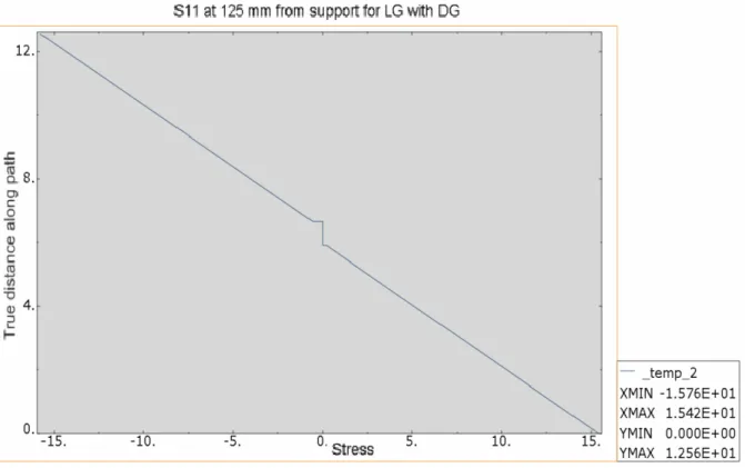
Following two plots show the stress (S11) distribution along mid section and at 125 mm from support. The behaviour is similar to LG with Solutia DG interlayer. Highest tensile stress is found at the bottom edge of bottom glass plies and highest compressive stress at the top edge of the top glass. Table 5.13 presents magnitude of maximum tensile and compressive stresses along depth (bottom and top face of each glass plies) in middle section of LG beam. It is clear from that Table 5.13 and from Figure 5.19 and 5.20 that this type of LG unit also behaves more similar to a monolithic unit.
Figure 5.19 Stress S11 along mid-section for LG with Sentry glass
Table 5.13 Maximum tensile and compressive stresses along depth for LG with Sentry Glass
Distance from bottom edge in mm Maximum tensile and compressive stresses in MPa
0 27.31
5.93 - 5.47
6.82 7.67
12.74 - 40.42
Figure 5.21 Stress concentration for LG with Sentry Glass in middle part
Following plots (Figures 5.22, 5.23 and 5.24) represent load versus displacement curve from experimental test and from FE model for all specimens in a single plot. Figure 5.22 presents plot for full load range whereas Figure 5.23 presents initial stiffness slope (10 to 100 N) part from experiment. The load versus displacement plots from ABAQUS (Figure 5.24) show linear behavior for all specimens.
Figure 5.22 Force versus displacement plot for experimental value
Figure 5.24 Load versus displacement for different specimen from ABAQUS model Figure 5.25 presents load versus maximum principal stress plot from FE model results for all specimen in a single plot for comparison between the different specimens. It shows that LG with PVB is the least stiff unit whereas LG with Sentry glass is stiffest among the three types of LG. It is also noticeable in the plot from experiment for full load range (Figure 5.22). But in load versus displacement plot from ABAQUS model result data (Figure 5.24) and initial stiffness slope (Figure 5.23) plots show that LG with PVB has highest slope. This is because the effective length was less for that type of LG than the other two. Another important reason is that the behavior of PVB depends on time (loading rate).