WORKING PAPER
05/2014
Costs of traffic accidents with wild boar populations in Sweden
aTobias Häggmark.Svensson, aIng-Marie Gren, aHans Andersson, bGunnar Jansson, cAnnika
Jägerbrand
Economics
aDepartment of Economics, Swedish University of Agricultural Sciences, Uppsala bGrimsö Wildlife Research Station, Department of Ecology, Swedish University of
Agricultural Sciences, 730 91 Riddarhyttan
cEnvironmental Unit, Swedish National Road and Transport Research Institute, Box 55685,
10215 Stockholm
Sveriges lantbruksuniversitet, Institutionen för ekonomi Working Paper Series 2014:05 Swedish University of Agricultural Sciences, Department of Economics Uppsala 2014
ISSN 1401-4068
ISRN SLU-EKON-WPS-1405-SE Corresponding author:
Tobias.haggmark@slu.se
Costs of traffic accidents with wild boar populations in Sweden
Abstract: Traffic accidents with wild boar have increased rapidly over the last years in Sweden. This paper calculates and predicts costs of current and future accidents, totally and for different Swedish counties, based on estimates of wild boar populations. A logistic population model is assumed, and econometric methods are used for calculating populations with panel data on traffic accidents, traffic load, and landscape characteristics for each county. The results show an average growth rate of 0.48, which varies between 0.39 and 0.52for different counties. This, together with predictions on changes in traffic load, forms the basis for calculations of costs of traffic accidents for a 10 year period. In total, the
predicted costs can increase from 60 million SEK in 2011 to 135 or 340 million SEK in 2021 in present value depending on hunting pressure. The variation in cost increases is, however, large among counties, increasing by tenfold in Stockholm and Södermanland where the wild boar populations are relatively small and by approximately 50% in counties with mature populations.
Key words: traffic accidents, costs, wild boar, econometrics, land scape characteristics, Sweden.
JEL codes: Q29, Q57
Department of Economics Institutionen för ekonomi
Swedish University of Agricultural Sciences (SLU) Sveriges lantbruksuniversitet P.O. Box 7013, SE-750 07 Uppsala, Sweden Box 7013, 750 07 Uppsala
Ph. +46 18 6710 00, Fax+ 46 18 67 35 02 Tel. 018-67 10 00, fax 018 67 35 02
www.slu.se www.slu.se
1.Introduction
The numbers of wild boar traffic accidents in Sweden have increased continuously during the latest decade. For example, between 2003-2011 the reported number of traffic accidents increased by approximately 250% (Nationella Viltolycksrådet, 2013; Jägerbrand, 2012). Due to the relatively low height of wild boars drivers seem to have difficulties in detecting the animals on or close to the road. Wild boars often travel in groups and vehicle collisions with several animals may cause more damages. Furthermore, the low angle of impact at collision and the heavy weight of wild boars give, in general, rise to more serious vehicle damage than compared to e.g. deer collisions. Despite the national and international concern for wild life traffic accidents, and the scientific community’s long term experience from ecological modelling of impacts of wild life on, among other, traffic accidents, there is, to the best of our knowledge, no study estimating costs of traffic accidents with wild boar in Sweden. In principle, it would be relatively easy to calculate such costs by simply multiplying the number of traffic accidents from wild boar with the cost per accident. However, this would not allow us to predict future cost from expected increases in the size of the wild boar population. Furthermore, the expected increases of the populations differ among regions in Sweden because of varying landscape and climate characteristics. The purpose of this study is to calculate and predict dynamic and spatial dispersion of costs from traffic accidents by estimating wild boar population using a model that accounts for differences in land-scape characteristics among regions.
Naturally, one important reason for the increase in traffic accidents is the rapid increase of the wild boar population. The hunting bag statistics show an annual mean increase of ca 30% during 2000-2010 in Sweden, and the biological growth rate was estimated to ca 48% in the same period (Lemel and Truvé, 2008; Jansson et al., 2011). However, according to Tham (2004) wild boars have existed in Sweden over thousand years. They were eradicated in the end of the
seventeenth century but reinstated in 1723 for hunting purposes on the island Öland. This caused protests among farmers and they were again eradicated in the end of 1770. Once again minor populations were kept in enclosures but some individuals escaped in the 1970’s, and the wild boar population reestablished itself. The wild boar population was accepted as part of the Swedish fauna by the parliament in 1988 (SFS 1987: 905).
There is a relatively large body of literature on costs and benefits of measures curbing traffic accidents with wildlife, such as fences, road tunnels, and warning signs (e.g. Seiler, 2004; 2005; Hussain et al., 2007; Huijser et al., 2009). A common approach has been to derive the impact of mitigation measures on accidents by statistical analysis. The role of landscape characteristics for traffic collisions with deer has been investigate by Hussain et al. (2007), who used a panel data set for explaining collisions in different counties in Alabama, USA. A similar study using landscape attributes, traffic load etc. to assess and predict risk zones for ungulate-vehicle collisions in Sweden was conducted by Seiler (2004, 2005). Huijser et al. (2009) calculated costs and benefits from measures such as fences along motor ways and speed limits which reduce the number of collisions with large ungulates (elk, moose, and deer) in USA and Canada.
However, these cost and benefit calculations of mitigation measures do not include wildlife population dynamics, which is necessary when aiming to predict future costs of traffic accidents. Wildlife population models are numerous in the ecological literature, with a variety of scopes and methods. Commonly used background data or methods are, for example; hunting statistics, capture-recapture, indirect indices, line-transect surveys of tracks or pellets and direct observation at feeding sites (Avecedo et al., 2007). The most common approach to estimate ungulate populations of extensive areas, like counties or nations, has been to use bags statistics. This was used to estimate the Swedish wild boar population in 2005, resulting in ca 40 000 animals (Svenska Jägarförbundet 2010), which was believed to exceed 150 000 animals 2010 (Jansson et al. 2011).
Boitani et al. (1995) employed a catch per unit of effort method in an attempt to estimate the wild boar population in Tuscany (Italy). This approach requires good information regarding the amount of effort put in to capturing the animals and that the population is closed during capturing events. It is not plausible to enclose the population or to conduct a capture-recapture study at a larger scale. Geisser and Reyer (2005) studied the wild boar population density in Thurgau (Switzerland), where hunting statistics, road accidents and various ecological factors were analysed by principal component analysis and stepwise regression to obtain a population density index. Their study showed that an increased population density is correlated to traffic accidents, and that the population density to some extent depends on, and in some cases significantly related to, ecological factors.
The problem in our case with using hunting statistics is the lack of appropriate effort variables, such as number of hunters and time spent on hunting wild boars. Such an effort variable is not available at the county level, in Sweden. Therefore, this study makes use of data on traffic accident for different counties during the period 2003-2012 with different formulations of traffic load as a measure of effort. The relationship between traffic load and wildlife accidents has previously been described (Seiler, 2004), who also pointed out the role of landscape characteristics. Our approach and dataset also allows for the estimation of the impacts of landscape characteristics on growth of wild boar populations in different counties. The theoretical basis rests on long term experiences from estimation of fish populations, with a common assumption of a logistic functional form (Schaefer, 1954). To the best of our knowledge, the approach of using road kills to estimate population development and costs of traffic accidents involving wildlife has not been applied by any earlier study. In our view, a contribution of this paper is thus the development and application of data on traffic accidents for approximating wildlife populations. In addition, we estimate and predict costs of traffic accidents with wild boars in Sweden accounting for differences in landscape characteristics among counties, which has not previously been carried out.
The paper is organized as follows. First, we present the theoretical framework for estimating wild boar populations based on data on traffic accidents and traffic load. Section 3 shows data retrieval and results from the statistical analyses. Calculated and predicted costs of traffic accidents from wild boars are presented in Section 4. The paper ends with a summary and conclusions.
2. Theoretical background for calculations and predictions of wild boar
populations
Following the literature in fishery economics (e.g. Shaefer, 1954; Kataria, 2007), it is assumed that the development of wild boars over time in each county i, where i =1,..n counties, depends on population growth, traffic accidents, and hunting. The population growth is assumed to follow a logistic function, which is written as:
i t i t i i t i t i i t V H K P P r t P − − − = ∂ ∂ 1 (1) where i t
P is population in period t, ri is the intrinsic growth rate, Ki is the maximum population
without hunting and traffic accidents, i t
V is individuals killed in traffic accidents, and i t
H is hunting.
Traffic accidents, in turn, are assumed to depend on traffic load, i t
T , and a coefficient, ai, relating
accidents to the traffic load and i t P , which is written as i t i t i i t a T P V = (2) 7
Equation (2) thus shows that the number of killed animals from traffic accidents can be calculated when i
t
P , ai, and i t
T are quantified. Since we don’t have information on i t
P and ai
they are estimated by assuming that accident per unit of traffic load, i t S , is proportional to the population where i t i t i t S T V = (3)
which is used to derive regression equations that can be estimated with statistical tools. However, landscape characteristics, i
t
L , are not accounted for in (1). In principle, these can enter the population dynamics in two ways; directly as an additional variable in a similar way as i
t
V and i
t
H , or indirectly on the impact on the intrinsic growth parameter, ri.
Direct impacts of landscape characteristics are formulated as effects on population growth according to i t i i t i i t i t i i t i t V f L K P P r H t P − + − = + ∂ ∂ 1 (4)
where fi reflects the marginal impact on population growth of landscape characteristics i t
L .
It is now assumed that a proportional change in population can be approximated by a proportional change in accidents per unit traffic load. The latter is obtained by replacing i
t
P in
equation (4) with i t i t i t i i t T V P a
S ≡ = in equation (3), writing the left hand side of (4) accordingly as
) ( i t i H t P a + ∂ ∂ , and dividing by i t S , which gives i t i t i i t i t i t i i t i i i i t i t S L f S H T a S K a r S t S + + − − = ∂ ∂ ) ( 1 (5)
The derivative in the dependent variable is obtained by making a finite difference approximation according to 2 1 1 − + − = ∂ ∂ t St St t S (6)
The regression equation for population growth with direct impacts of landscape characteristics is then specified as iD t i t i t i i t i t i t i i t i i i t S L S H T S Y =α 1+α 2 +α 3( + )+α 4 +ε (7)
where the correspondence of coefficients in equation (7) with those in equation (5) are
i i i i i i i i i i t i t i t i t a f K a r S S S Y = = = = − = − + 4 3 2 1 1 1 , , 1 , , 2 α α α α
We can now calculate carrying capacity as the population level where eq. (5) equals zero without any hunting and accidents and recognizing that i
t i i t a P S = , which gives 9
3 2 4 i i i t i i i r L K α α α + = (8)
With respect to the indirect specification, it is assumed that the intrinsic growth rate shows a linear dependence on landscape characteristics, i
t i i
i b c L
r = + . The wild boar population growth equation can then be written as
i t i t i i t i t i t i i i t V H K P P L c b t P − − − + = ∂ ∂ 1 ) ( (9)
Following the same assumption and steps as for the direct specification gives population unit growth rates as ) ( 1 i t i t i t i i t i i i t i i i t i t S H T a S K a L c b S t S + − − + = ∂ ∂ (10)
The regression equation is then specified as
iID t i t i t i t i i t i i t i i i t S H T S L Y =α 5 +α 6 +α 2 +α 3( + )+ε (11) i t i i i L r =α 5 +α 6 and i t
Y , αi2, and αi3 are defined in the same was as for the direct specification. The intrinsic
growth rate, i
t i i
i L
r =α 5 +α 6 , varies over time and among counties because of i t
L . Carrying capacity is calculated for the population level where (9) equals zero without any hunting or traffic accidents, i.e. i
t i i S r 2 0= −α and i t i i t a P S = , which gives 10
2 i i i iI a r K α = (12)
Predictions of future accidents requires forecasts of future populations, and they are, for both the direct and indirect models, found by integrating the logistic population growth model in (1) with respect to time. However, traffic accidents and hunting may give create difficulties in finding solutions, and we therefor transform equation (1) into a more simple representation where traffic accidents and hunting are expressed in terms of a proportion, zi, of the population, which is
written as i t i i i t i t i i t z P K P P r t P − − = ∂ ∂ 1 (13)
where zi is the combined relative decline in population from both accidents and hunting. We can then use one form of solution for a non-linear first-order differential equation (e.g. Matthews, 2014), which gives t z r i i i i i i i i i i i t i i e P K z P K r r K z r P ) ( 0 0) ( ) ( − − − − + − = (14) where − → i ii i t r z K P 1 when t→∞.
Thus, future populations can be determined for different levels of pressures zi when estimates of intrinsic growth rates, carrying capacity, a base year population, i.e. Pi
0 , are available.
3. Data retrieval and estimation of regression equations
The two regression models in eq. (7) and (11) constitute the basis for the numerical approximation of wild boar populations, and subsequent calculations of costs of traffic accidents in different counties in Sweden. In this section we therefore give backgrounds with respect to data collection, and estimation of these regression equations.
3.1 Data retrieval
The data needed for estimating regression equations specified in equation (7) and (11) are; traffic accidents, traffic load, animals killed by hunting, and landscape characteristics. In this study we make use of a panel date set on these variables which includes 13 counties with wild boar populations during the period 2003-2012 (Nationella Viltolycksrådet, 2013). During this period the number of traffic accidents with wild boar has increased six fold from approximately 750 to 4100 (Figure 1).
Figure 1: Traffic accidents from wild boar over 2003-2012 Source: Nationella Viltolycksrådet (2013)
752 666 984 1013 1576 2452 3076 2432 2627 4153 0 500 1000 1500 2000 2500 3000 3500 4000 4500 2003 2004 2005 2006 2007 2008 2009 2010 2011 2012 W ild B oa r A cci den ts 12
The data on wild boar accidents, as collected by the Nationella Viltolycksrådet (2013),are to be considered as relatively accurate. Since 1987 drivers are obliged by §40 Jaktförordningen to report to the authorities if they are involved in a wildlife accident and injuring the animal. Further, since 2010 it is compulsory for vehicle drivers to report the accident to the police even if the animal is not hurt. However, according to Leisner and Folkesson (2006) the non-reported number of accidents may be significant, the consequences of which are discussed in Section 4 where we present the population calculations.
Traffic accidents are distributed heterogeneously among the counties, and the highest levels are found in the southern county Skåne (Figure2).
Figure 2: Average number of traffic accidents over 2003-2012 in different Swedish counties Source: Nationella Viltolycksrådet (2013)
The number of animals killed by traffic accidents corresponds to approximately 5% of those killed by hunting, which increased during the period 2003-2012 from approximately 17000 to 97000 (Viltdatabasen, 2014). The relative change is thus in the same order of magnitude as the relative increase in traffic accidents. The allocation of killed animals by hunting among counties also follows the same pattern as that of traffic accidents (Figure 3).
0 100 200 300 400 500 600 N um ber o f t ra ffi c ac ci den ts 13
Figure 3: Average number of killed animals from hunting over 2003-2012 in different Swedish counties
Source: Viltdatabasen (2014)
However, when we relate the number of animals killed by traffic accidents presented in Figure 2 to traffic load the pattern changes (Figure 4). Traffic load is measured in millions of kilometers driven in each county (Trafik Analys, 2013a,b). This statistical measure does unfortunately not include foreign traffic, which will underestimate the true amount of kilometers driven, and thereby overestimate the accident intensities presented in Figure 4.
Figure 4: Traffic accidents per traffic load in million driving km. Source: Nationella Viltolycksrådet (2013), Trafik Analys (2013a,b)
0 1000 2000 3000 4000 5000 6000 7000 8000 9000 10000 Kille d a nim als 0 0,2 0,4 0,6 0,8 1 1,2 1,4 1,6 14
The largest number of accidents per traffic load occurs in Kalmar county, where it is almost 50% higher than in the county with the second largest number of accidents per traffic load. The Skåne county has the largest number of wild boar accidents but shows a relatively low accident intensity. The variations in intensities can be explained by the presence of wildlife fences along certain roads but also by landscape characteristics which promote growth of wild boar population.
In this study we therefore include the length of fences as explanatory variable measured as the length of the fences in relation to the road kilometers in the county i.e. a ratio between the two. Included landscape characteristics are: areas of deciduous and boreal forests, pasture, and arable land. A deciduous component, specially beech (Fagus) and oak (Quercus), of the forest is appreciated by wild boars, and generally regarded to promote population development (Markström & Nyman, 2006). Detailed data on tree species composition, i.e. here to discern the occurrence of these broadleaved stands, are however not available for the period under study why we confine the forest habitat parameter to separate only between deciduous and coniferous forest. Both pastures and arable land constitute important feeding sites for wild boar (Markström & Nyman, 2006), and the distribution of such habitats may naturally influence their movements, especially crop fields in late summer (Jansson et al., 2012). However, although these habitats are attractive per se, the size and shape of such fields are also important, where small and narrow fields are preferred by wild boars rather than large open areas (Jansson et al., 2011).
It should also be recognized that deciduous forest, as well as other types of forest, may provide some difficulties for drivers to detect movements of wild boars in the landscape and thereby, ceteris paribus, increasing the probability of an accident but the problem is less accentuated for deciduous forest. On the contrary, arable and pasture land with a more open type of landscape tend to improve visibility thereby reducing the risk of an accident. However, a more open type of landscape would be less attractive to the wild boars that often tend to congregate in the intermittent area of forest and open landscape elements. Hence, we would expect a negative sign for the variables arable and pasture land.
In Sweden, supplemental feeding of wildlife, mainly ungulates, is allowed and extensively applied in many areas. For wild boar, this is part of the management (for hunting and/or to lure them from crop fields) and feeding stations are often frequently utilized and generally believed to promote its reproduction (Bergqvist & Pålsson, 2010). Thus, we are well aware of that the extent (volumes and frequency) and distribution of supplemental feeding stations may confound the otherwise expected relationship between population development and habitat/landscape type, as well as influencing the local movements of wild boar. However, neither the number of feeding stations nor their positions are registered, why we in this study are not able to include them in our estimates. The estimates of the population dynamics will then be biased upwards for counties with relatively much feeding.
We construct two different specifications of the effort variable in terms of traffic load, 𝑇𝑖, 𝑖 =
1,2, where 𝑇1is specified as 𝑅𝑜𝑎𝑑 𝑎𝑟𝑒𝑎 𝑖𝑛 ℎ𝑎𝑇𝑟𝑎𝑓𝑓𝑖𝑐 𝑙𝑜𝑎𝑑 , and 𝑇2 as 𝐶𝑜𝑢𝑛𝑡𝑦 𝑠𝑖𝑧𝑒𝑖𝑛 1000 ℎ𝑎𝑇𝑟𝑎𝑓𝑓𝑖𝑐 𝑙𝑜𝑎𝑑 . Because of these two
specifications of traffic load we will have two constructs of i t
S and i t
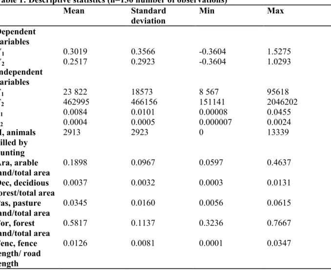
Y respectively. We add fences as a control variable which affects number of accidents but not population per se. Descriptive statistics of all variables are presented in Table 1.
Table 1: Descriptive statistics (n=130 number of observations)
Mean Standard
deviation Min Max
Dependent variables Y1 0.3019 0.3566 -0.3604 1.5275 Y2 0.2517 0.2923 -0.3604 1.0293 Independent variables T1 23 822 18573 8 567 95618 T2 462995 466156 151141 2046202 S1 0.0084 0.0101 0.00008 0.0455 S2 0.0004 0.0005 0.000007 0.0024 H, animals killed by hunting 2913 2923 0 13339 Ara, arable land/total area 0.1898 0.0967 0.0597 0.4637 Dec, decidious forest/total area 0.0037 0.0032 0.0003 0.0131 Pas, pasture land/total area 0.0345 0.0160 0.0056 0.0615 For, forest land/total area 0.5817 0.1137 0.3236 0.7667 Fenc, fence length/ road length 0.0126 0.0081 0.0001 0.0347
3.2 Regression equations and results
The data set is a panel with observations for 13 counties over the period 2003-2012. We therefore test for fixed or random effect model, and if a random effect model is statistically better than an ordinary least square estimate. In order to verify that the relationship should be represented by a random effects model, compared to a fixed effects model, the Hausman test is used (appendix A, Table A2). The observed p-value for the tests indicated that the null-hypothesis cannot be rejected, favoring a random effects model. However, according to the
Breusch-Pagan-Lagrange multiplier test the model can be reduced to an ordinary least squares (OLS) regression model, instead of a random effects model. Hence the produced result is estimated using OLS regression models.
Tests indicated the presence of heteroscedasticity and we therefore estimated all four models, i.e. the two models specified in equations (7) and (11) with two different effort variables, with robust standard errors. However, all variables on landscape characteristics presented in Table 1 could not be included in the estimation due to multicollinearity. By removing some variables we managed to get an acceptable mean variance inflation factor of 1.11 and 1.10 for model 1 and model 2 respectively. The regression equations were then specified as:
Indirect model: k it it k it k it k k it k k it it k it k k k
it T H S S Ara Dec Fenc
Y =α 1+α 2( + / )+α 3 +α 4 +α 5 +α 6 +ε (15) Direct model: k it it k k it it k k it it k k it k k it it k it k k k
it T H S S Ara S Dec S Fenc
Y =β 1+β 2( + / )+β 3 +β 4 / +β 5 / +β 6 +υ (16) where k=1,2 for the two measures of Tit.
In order to make statistical comparisons of the model specifications the Akaike Information Criterion, AIC, is used where the model with the lowest AIC value (𝐴𝐼𝐶𝑚𝑖𝑛) is to be considered
preferable. Table A6 in appendix A shows the information relevant for Model 1 and Model 2. According to delta AIC, ∆𝑖, which is less than 2, the models which have 𝐴𝐼𝐶 > 𝐴𝐼𝐶𝑚𝑖𝑛 can be
considered to have a satisfactory fit and there exists substantial evidence for the model specifications, i.e. the difference between the models is small and it is not possible to distinguish between the two. However when computing the parameters relevant for the wild boars and the population size, the indirect model produces the most plausible result, and we therefore present
this model in the main text. The relative information loss between the models is to be considered small.
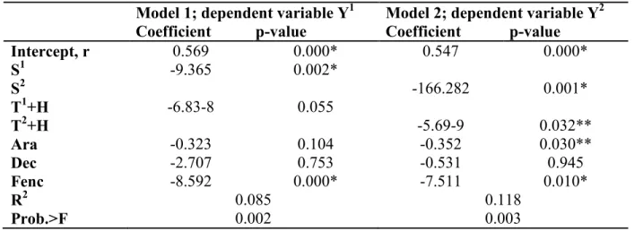
Table 2: Regression results of the logistic models
Model 1; dependent variable Y1
Coefficient p-value Model 2; dependent variable Y
2 Coefficient p-value Intercept, r 0.569 0.000* 0.547 0.000* S1 -9.365 0.002* S2 -166.282 0.001* T1+H -6.83-8 0.055 T2+H -5.69-9 0.032** Ara -0.323 0.104 -0.352 0.030** Dec -2.707 0.753 -0.531 0.945 Fenc -8.592 0.000* -7.511 0.010* R2 0.085 0.118 Prob.>F 0.002 0.003 Significance Level: *=p<0.01, **=p<0.05, ***=p<0.1
All statistically significant estimates show expected signs; the traffic effort variable including hunting (T1+H, T2+H) is negative, the accident intensity (S1, S2) is negative, Fenc is negative,
and the intercepts, the intrinsic growth rates, are positive. The landscape characteristics could have either sign, the significant negative coefficient of the share of arable land, Ara, can be explained by relatively large areas without hiding opportunities in the landscape, which is avoided by the wild boar. It is interesting to note that the construction of fences has, in average, decreased the annual increment in accidents by approximately 8-9%. Without the fences, the accidents in relation to traffic load would thus have increased by approximately 30% more than the averages of 0.30 and 0.25 presented in Table 1.
Unfortunately the models do not have a high R2 value indicating that some variation has not been
accounted for. On the other hand, the F-values are significant at the 5% confidence level. Since almost all coefficients are significant in Model 2, and the R2 is somewhat larger than that for
Model 1, we use results from Model 2 in the subsequent calculations. Furthermore, since only 19
share of arable land is significant we use this when calculating the intrinsic growth rates, totally and for each county. In average for total Sweden, this corresponds to the value of the intercept of Model 2 in Table 2, 0.547, minus the estimated coefficient of -0.352 times the average share of arable land, which from Table 1 is 0.1898. This gives an average intrinsic growth rate of 0.48, which is the same as that obtained by Lemel and Truvé (2008) and Jansson et al. (2011).
The estimated coefficient for the effort variable allows for the calculation of populations for the years 2004-2011 for which we have data on traffic accidents. The calculations are made
according to it it it it it it it it it it it a T VH S H aT VV H H P + + = + + = ) ( ) ( ) / ( 2 (17)
The calculated results are presented in Table 3.
Table 3: Calculated populations in different counties over the years 2004-2011
2004 2005 2006 2007 2008 2009 2010 2011 Blekinge 1451 1349 1429 2730 3177 8267 5870 3681 Halland 1806 2268 2107 2980 4079 6539 5560 4481 Jönköping 1602 1483 1587 2557 6087 6839 5445 5387 Kalmar 3630 4518 3864 9325 18985 26361 17277 18310 Kronoberg 8995 11903 20638 25445 30416 30750 20712 28416 Skåne 7945 8689 8169 12889 19202 21130 19537 21067 Stockholm 1271 1940 2282 2874 4907 5118 4855 5591 Södermanland 5220 7803 6390 9845 12893 14010 12396 14199 Uppsala 903 1467 2841 2982 3682 6454 3226 4986 Västmanland 328 506 2480 1541 1858 3243 3673 4648 Västra Götaland 254 714 149 499 1804 2923 2022 2841 Örebro 1121 1558 2194 2516 3321 6406 2792 4773 Östergötland 1511 3151 2635 4399 9738 12369 8651 8231 Total 36037 47349 56765 80582 120149 150409 112016 126611 20
According to our calculations, the total population shows an almost fourfold increase during the period 2004 to 2011, and amounted to approximately 126 000 animals in 2011. The relative increases have been particularly large in Västmanland and Västra Götaland where the population has increased more than ten times. When comparing the estimates with the few existing other estimates, it can be noted that the number for 2005 is close to the level of 40000 suggested by Swedish Jägarförbundet (2010), but a little bit lower for the year 2011 than the report of 150000 by Jansson et al. (2011).
However, our estimates can be biased because of the existence of unreported accidents. According to Seiler and Folkesson (2006) the factor relating unreported to reported accidents involving damage to property amounts to 0.6 for moose and deer. Similar estimates are not carried out for wild boar. If the factor is in the same order of magnitude as for moose and deer, our calculations of wild boar population can be considerably underestimated.
4. Cost of traffic accidents from wild boar populations
Costs of traffic accidents from wild boar accidents for each county are calculated as unit cost per accidents times the number of accidents. There exist no official statistics on unit cost of traffic accidents. In this study, data on average costs of accident including a wild boar have been obtained from an insurance company (Länsförsäkringar, 2014). These data indicate that the cost for a wild boar accident is roughly 23 000 SEK. Relating this to costs of accidents with other animals, the cost for roe deer and elk is 22000 and 38000 SEK respectively, it is apparent that a collision with wild boars can cause a lot of damage to the car. Fortunately it is rare to see damage to the people traveling in the car, and will thus not be included in this study.
The predicted number of accidents is estimated based on equation (2) in Section 2, i.e.
t t i t i t aT P
V = , which implies a need for predictions of traffic load, i t
T , and wild boar populations, 21
t t
P . Traffic loads by cars are expected to increase by 2% per year for all counties, but the deviations from the mean can be large (Trafikverket, 2014). The highest annual increase, 2%, is expected to occur in Stockholm , and the smallest, approximately 0.1%, in Gotland, see Table B5 in appendix.
Predictions of future wild boar populations are based on equation (14) in Section 2, which requires estimates of carrying capacity, Ki, intrinsic growth rates, ri, and base year populations,
i
P0 . Intrinsic growth rates are calculated by using equation (11) in Section 2 and the results
presented in Table 3 in Section 3. Carrying capacity is calculated by recognizing that the ai
coefficient includes both effort and animals killed by hunting. The effort is approximately 1/12 of the total reduction in each year, and we have therefore adjusted the ai coefficient in order to
capture this effect. The results are presented in Table 4.
Table 4: Intrinsic growth rate, and max population from regression results of Model 2
Counties Intrinsic Growth Rate Max population
Blekinge 0.501 53042 Halland 0.471 49866 Jönköping 0.511 54100 Kalmar 0.502 53148 Kronoberg 0.524 55477 Skåne 0.389 41184 Stockholm 0.498 52724 Södermanland 0.470 49760 Uppsala 0.464 49124 Västmanland 0.468 49548 Västra Götaland 0.471 49866 Örebro 0.494 52301 Östergötland 0.478 50607 Total 0.48 660745 22
According to our calculations, the wild boar population has a potential to grow by approximately 260% from the 2011 level. The intrinsic growth rates differ, being lowest for Skåne and highest for Kronoberg county.
Assigning Pi
0 at the population levels in 2011 (Table B1 and B2 in appendix B) and using the
intrinsic growth rates and carrying capacities in Table 4 we can predict i t
P and total population in Sweden, P , for future years (see equation (14) in Section 2). There is also a need for t
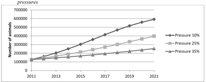
assumptions on hunting pressure on the population. In order to compare the results with respect to these pressures, we present calculations for three different pressures; 10%, 25% or 35% of the population is reduced every year. Given these assumptions, the predicted development of total populations over the 10 subsequent years are as displayed in Figure 4.
Figure 4: Calculated and predicted total wild boar population under different hunting pressures
Source: Tables B1-B3 in appendix B
The prediction is done for the years 2012 and 2013 as well due to the loss of observations in the estimation procedure. The total increase in the population over the 10 year period ranges between 50% and 390% depending on hunting pressure. However, exogenous factors can cause
0 100000 200000 300000 400000 500000 600000 700000 2011 2013 2015 2017 2019 2021 N umb er o f a ni ma ls Pressure 10% Pressure 25% Pressure 35% 23
this prediction to become inaccurate i.e. extremely harsh winters will cause the population to deviate from the prediction.
The forecasted developments of the population in different counties show considerable differences (Figure 5).
Figure 5: Predicted increases in population from the 2011 level to 2012 for different counties and hunting pressures.
Source: Tables B1-B3 in appendix B
Irrespective of hunting pressure, the largest increases as measured in percent from the 2011 level occur in counties with relatively low population levels in this year, e.g. Blekinge and Västra Götaland, where the populations can show a tenfold increase. For these counties the level of hunting pressures has large effect of the population and its growth. When the hunting pressure corresponds to 35% of the population level each year, the predicted increases are reduced to a doubling of the population.
The predictions of population increases presented in Figure 5 provide the basis for the determination of future traffic accidents. We also need to consider expected changes in traffic
0 200 400 600 800 1000 1200 % c ha ng e
10% pressure 25% pressure 35% pressure
load, the annual increase of which varies between 0.001 and 0.02 between different counties (Table B5 in appendix). The combined effect of growths in wild boar populations and traffic load on total traffic accidents is presented for different years in Figure 6.
Figure 6: Predicted development of total traffic accidents over 2011-2021
Source: Tables B5-B7 in appendix B
The predicted number of total accidents in 2012 and 2013 under the assumed low pressure corresponds to, respectively, 3483 and 4493 (Table B5). These figures can be compared with the actual number of 4170 in 2012 and 3551 in 2013 (Nationella Viltolycksrådet, 2014). The average number of predicted accidents between these years, 3988, is then relatively close to the actual average of 3860, although the precision in prediction for each year is not so high.
The difference is large between the predicted number of traffic accidents depending on assumption of hunting pressure; it can very between approximately 6900 and 16300. The variation is also considerable between different counties (Figure 7).
0 2000 4000 6000 8000 10000 12000 14000 16000 18000 2011 2013 2015 2017 2019 2021 N um ber o f t ra ffi c ac ci den ts Pressure 10% Pressure 25% Pressure 35% 25
Figure 7: Predicted increases in traffic accidents from 2011 level in % for different counties and hunting pressures
Source: Tables B5-B7 in appendix B
The predicted increases in traffic accidents follow to some extent those in populations, but can be either reinforced or counteracted by the increases in traffic load. For Blekinge, population has the largest increase but traffic load increase is relatively low and the combined effect show that the increase can range between 210% and 1150%. The reverse is the case for Stockholm county, and the percent increase in accidents is then predicted to be larger than the corresponding increase in the wild boar population. However, the corresponding range in the total increase is considerably lower, between approximately 100% and 500%, because of the low increases in counties with relatively large populations, Kalmar, Kronoberg, and Skåne.
When calculating costs of the traffic accidents presented in Figures 6 and 7 we also have to assign a value of the discount rate. There is a large debate on the correct level of the social discount rate, but recommendations range between 1% and 5% depending on time perspective (e.g. Boardman, 2010). We use the level on 2% in our calculations and assign the cost of SEK 23000 per accident, which give the development of costs under different pressures as shown in Figure 8. 0 200 400 600 800 1000 1200 1400 1600 % in cr ea se
10% pressure 25% pressure 35% pressure
Figure 8: Predicted development of costs in present value of traffic accidents under different hunting pressures, total for Sweden
Source: Calculations based on Table B5-B7 in appendix B, 2% discount rate, and a cost of SEK 23000/accident
In 2011 the total number of traffic accidents was 2627, and with an average cost of 23000 per accident the total cost amounted to approximately 60 million SEK. Depending on hunting pressure this cost can increase to 135 or 320 million SEK in 2021. Each of the three different cost paths corresponds to a sum of discounted annual costs which amounts to 0.9, 1.4, or 2 billion SEK over the 10 year period. Recall that the cost is calculated as the expenses for insurance companies. Hunting pressures of 25% or 35% would then save expenses for the companies corresponding to 0.5 or 1 billion SEK compared with a pressure of 10%. The insurance companies would thus have an incentive to pay for increased hunting.
A further investigation of where these predictions of total cost increases occur, show that they are unevenly divided among counties (Figure 9).
0 50 100 150 200 250 300 350 2011 2013 2015 2017 2019 2021 M illio n S EK/ ye ar 10% pressure 25% pressure 35% pressure 27
Figure 9: Predicted increases in annual costs of traffic accidents from 2011
to 2021 in different counties and hunting pressures, million SEK in present value.
Source: Calculations based on Table B5-B7 in appendix B, 2% discount rate, and a cost of SEK 23000/accident
The largest annual costs increases occur in Stockholm and Södermanland county where they can amount to approximately 35-40 million SEK, which is explained by the relatively large increase in population or traffic load. The results in Figure 9 thus give some insights into the spatial targeting of hunting if reduction in traffic cost is an objective for wild boar management. The largest cost savings from a given increase in hunting in early years are likely to be obtained for the two counties with the largest predicted cost increases.
5.
Summary and conclusions
The purpose of this study has been to estimate and predict costs of traffic accidents with wild boar in Sweden. The aim of predicting traffic costs required information on the development of
0 5 10 15 20 25 30 35 40 45 M illio n S EK
10% pressure 25% pressure 35% pressure
the wild boar population over time. Such population models were estimated for different counties by means of data on traffic accidents and traffic load. A crucial assumption in this estimation was that of a logistic function of the population dynamics. Another important assumption was that the population growth rate can be derived from the growth rate in traffic accidents per unit traffic load. Given these assumptions and a panel data set over the period 2003-2012 for 13 counties we estimated population growth functions which accounted for differences in landscape characteristics among the counties. The calculated average intrinsic growth rate for Sweden amounted to 0.48, and it varied between 0.39 (Skåne) and 0.52 (Kronoberg). The calculated maximum population is approximately five times larger than current (2011) population levels. In order to predict future wild boar populations we also needed to make assumptions of hunting pressure, and three levels were assigned; 10%, 25% or 35% of the population killed by hunting each year. Given the estimated growth rates and expected increases in traffic load, the predicted costs can increase from approximately 60 million SEK in 2011 to 135 or 340 million SEK in 2021 depending on hunting pressure. The relative increases are highest in counties with relatively low populations in 2011, high population and traffic load growth rates. The county facing the highest increase is Stockholm, which amounts to approximately 40 million SEK in 2021 under low hunting pressure. This is almost as high as the total cost of 60 million SEK in 2011.
The cost increases may put burden on the insurance companies which can transfer such costs by charging a higher premium for having a vehicle insured. This will in the end affect more people than the ones actually involved in accidents. On the other hand, the costs can decrease considerably, by approximately 60% under higher hunting pressure. The results also give some indication on the targeting of measures reducing the population where, for a given mitigation effort, the largest decrease is obtained in Stockholm and Södermanland county.
However, the logistic functional form on the population dynamics assumed in our study has been criticized because of the neglect of composition of population cohorts, and the assumption of a constant intrinsic growth rate (e.g. Clark, 1990). Choices of other functional forms or models, such as age-structured models, might give other predictions of population developments. On the other hand, it would not be possible to estimate such functions based on data on traffic accidents, which instead need data on biological parameters such as reproduction and survival rates for different cohorts. Another factor affecting the results is the existence of unreported accidents. Although there is an incentive to report in order to obtain compensation from insurance companies, not all accidents might be reported (Leisner and Folkesson, 2006). Our population estimates are affected if the share of unreported accidents has changed over the included period; if it has increased there is an overestimation and vice versa.
Appendix A: Regression results
Table A1: Regression Results of the Direct Model
Variable Model 1 Model 2
Effort -0.000000122 -0.00000000833**
Accident per unit of effort (𝑺𝒕) -5.573927** -78.05831** Arable Land 0.0008024** 0.0000545** Deciduous Forest -0.0068416 -0.0004208 Fences 0.00342 0.0002431 Intercept 0.3595199*** 0.3071112*** Prob. > F 0.000 0.000 𝑅2 = 0.079 𝑅2 = 0.1252 Significance Level: *=p<0.1, **p=<0.05, ***=p<0.01 30
Table A2: Hausman Test for Fixed or Random Effect, Model 1 Indirect Specification Variable Fixed Random Difference S.E
Effort 0.0000000289 -0.0000000683 0.0000000971 0.000000111
Accident per unit of effort (𝑺𝒕) -8.981529 -9.365629 0.3840993 4.556775 Arable Land -2.567309 -0.3239128 -2.243396 4.617424 Deciduous Forest 33.31048 -2.706631 36.01711 68.66425 Fences -12.28954 -8.592073 -3.697468 11.61849 Test: 𝑯𝟎: 𝑫𝒊𝒇𝒇𝒆𝒓𝒆𝒏𝒄𝒆 𝒊𝒏 𝒄𝒐𝒆𝒇𝒇𝒊𝒄𝒊𝒆𝒏𝒕𝒔 𝒊𝒔 𝒏𝒐𝒕 𝒔𝒚𝒔𝒕𝒆𝒎𝒂𝒕𝒊𝒄 𝑝 = 0.9781
Table A3: Hausman Test for Fixed or Random Effect. Model 2 Indirect Specification
Variable Fixed Random Difference S.E
Effort -0.0000000062 -0.00000000569 0.00000000051 0.00000000587
Accident per unit of effort (𝑺𝒕) -157.3535 -166.2829 8.929406 85.42251 Arable Land -1.736539 -0.35192 -1.384619 3.755898 Deciduous Forest 42.73184 -0.5319168 43.26376 55.34918 Fences -14.70066 -7.511348 -7.189311 9.109928 Test: 𝑯𝟎: 𝑫𝒊𝒇𝒇𝒆𝒓𝒆𝒏𝒄𝒆 𝒊𝒏 𝒄𝒐𝒆𝒇𝒇𝒊𝒄𝒊𝒆𝒏𝒕𝒔 𝒊𝒔 𝒏𝒐𝒕 𝒔𝒚𝒔𝒕𝒆𝒎𝒂𝒕𝒊𝒄 𝑝 = 0.9233
Table A4: Hausman Test for Fixed or Random Effect. Model 1 Direct Specification
Variable Fixed Random Difference S.E
Effort -0.0000000211 -0.000000122 0.000000101 0.000000115
Accident per unit of effort (𝑺𝒕) -8.650386 -5.573927 -3.076458 3.949366 Arable Land 0.0004249 0.0008024 -0.0003774 0.0003947 Deciduous Forest -0.0201474 -0.0068416 -0.0133057 0.0094 Fences 0.187597 0.0034221 0.0153375 0.0108743 Test: 𝑯𝟎: 𝑫𝒊𝒇𝒇𝒆𝒓𝒆𝒏𝒄𝒆 𝒊𝒏 𝒄𝒐𝒆𝒇𝒇𝒊𝒄𝒊𝒆𝒏𝒕𝒔 𝒊𝒔 𝒏𝒐𝒕 𝒔𝒚𝒔𝒕𝒆𝒎𝒂𝒕𝒊𝒄 𝑝 = 0.4819 31
Table A5: Hausman Test for Fixed or Random Effect. Model 2 Direct Specification
Variable Fixed Random Difference S.E
Effort -0.00000000470 -0.00000000833 0.00000000364 0.00000000589
Accident per unit of effort (𝑺𝒕) -137.177 -78.05831 -59.11876 76.19104 Arable Land 0.0000444 0.0000545 -.0000101 0.0000203 Deciduous Forest -0.001231 -0.0.0004208 -0.00008102 0.0006 Fences 0.0010882 0.0002431 0.0008451 0.0006724 Test: 𝑯𝟎: 𝑫𝒊𝒇𝒇𝒆𝒓𝒆𝒏𝒄𝒆 𝒊𝒏 𝒄𝒐𝒆𝒇𝒇𝒊𝒄𝒊𝒆𝒏𝒕𝒔 𝒊𝒔 𝒏𝒐𝒕 𝒔𝒚𝒔𝒕𝒆𝒎𝒂𝒕𝒊𝒄 𝑝 = 0.4378
Table 6: AIC tests of Model 1 and Model 2 Number of
Parameters AIC Delta AIC (∆𝒊) Akaike Weight
Model 1: Indirect Specification 6 82.397 0 0.588 Direct Specification 6 83.112 0.71545 0.411 Model 2: Indirect Specification 6 37.188 0.81682 0.399 Direct Specification 6 36.371 0 0.601 32
Appendix B: Tables on population calculations, predictions of traffic load,
wild boar populations, and traffic accidents
Table B1: Predicted number of animals with 10% pressure
2012 2013 2014 2015 2016 2017 2018 2019 2020 2021 Blekinge 5314 7556 10534 14309 18827 23877 29103 34102 38534 42208 Halland 5670 7772 10443 13690 17429 21477 25576 29455 32897 35784 Jönköping 7728 10853 14828 19583 24871 30295 35416 39885 43527 46331 Kalmar 23136 28088 32782 36908 40302 42943 44913 46334 47337 48032 Kronoberg 33407 37745 41251 43920 45863 47229 48169 48804 49229 49511 Skåne 23490 25705 27658 29327 30715 31845 32746 33456 34008 34433 Stockholm 7906 10951 14772 19294 24287 29396 34234 38488 41993 44729 Södermanland 19346 25806 33542 42301 51610 60862 69463 76977 83193 88107 Uppsala 6862 9293 12326 15943 20025 24360 28673 32696 36228 39168 Västmanland 6441 8787 11750 15327 19418 23818 28249 32423 36116 39208 Va Götaland 4014 5611 7736 10472 13853 17824 22220 26776 31190 35192 Örebro 6718 9365 12754 16872 21568 26552 31452 35923 39732 42792 Östergötland 11780 15560 19947 24724 29577 34174 38247 41648 44351 46415 Total 161811 203093 250323 302670 358347 414653 468460 516967 558334 591909
Table B2: Predicted number of animals with 25% pressure
2012 2013 2014 2015 2016 2017 2018 2019 2020 2021 Blekinge 4637 5810 7233 8937 10942 13256 15866 18737 21806 24992 Halland 5464 6627 7990 9568 11368 13388 15611 18008 20536 23141 Jönköping 6783 8473 10485 12832 15506 18471 21661 24985 28335 31597 Kalmar 21049 23818 26531 29108 31485 33618 35488 37091 38440 39559 Kronoberg 30794 32886 34677 36175 37404 38395 39185 39807 40294 40672 Skåne 21739 22359 22928 23448 23919 24345 24728 25072 25378 25651 Stockholm 6945 8565 10470 12669 15152 17888 20823 23879 26969 29998 Södermanland 17078 20396 24164 28370 32977 37919 43101 48412 53724 58912 Uppsala 6021 7233 8638 10245 12055 14060 16242 18567 20994 23472 Västmanland 5645 6821 8193 9775 11570 13576 15775 18137 20619 23170 Va Götaland 3492 4279 5223 6345 7666 9201 10961 12945 15144 17531 Örebro 5885 7272 8919 10843 13049 15523 18232 21119 24110 27119 Östergötland 9889 11777 13889 16201 18676 21263 23897 26513 29044 31433 Total 145420 166315 189340 214515 241769 270902 301568 333272 365395 397247 33
Table B3: Predicted number of animals with 35% pressure 2012 2013 2014 2015 2016 2017 2018 2019 2020 2021 Blekinge 4231 4854 5558 6350 7236 8224 9317 10519 11831 13253 Halland 4998 5564 6184 6862 7601 8402 9268 10199 11195 12256 Jönköping 6214 7145 8191 9356 10646 12060 13599 15256 17021 18881 Kalmar 19838 21371 22891 24380 25823 27206 28518 29750 30897 31955 Kronoberg 29460 30396 31230 31967 32614 33178 33667 34089 34453 34764 Skåne 21110 21151 21190 21228 21265 21300 21334 21367 21399 21429 Stockholm 6368 7233 8193 9252 10413 11677 13042 14504 16056 17689 Södermanland 15710 17343 19105 20996 23017 25166 27437 29825 32319 34909 Uppsala 5517 6094 6721 7400 8134 8923 9768 10670 11629 12642 Västmanland 5166 5733 6352 7026 7758 8549 9402 10316 11291 12327 Va Götaland 3183 3561 3981 4446 4958 5522 6141 6818 7557 8358 Örebro 5386 6116 6928 7828 8820 9907 11090 12370 13744 15205 Östergötland 9125 10089 11123 12226 13394 14623 15907 17239 18611 20011 Total 136305 146650 157646 169317 181677 194736 208490 222923 238003 253681
Table B4: Predicted annual rates of increases in traffic load
County Rate Blekinge 0.007 Halland 0.015 Jönköping 0.010 Kalmar 0.005 Gotland 0.001 Kronoberg 0.014 Skåne 0.013 Stockholm 0.020 Södermanland 0.010 Uppsala 0.017 Västmanlnad 0.012 Va Götaland 0.011 Örebro 0.007 Östergötland 0.012
Source: Trafikverket (2014), Table 5
Table B5: Predicted number of traffic accidents with a pressure of 10% of the population 2012 2013 2014 2015 2016 2017 2018 2019 2020 2021 Blekinge 127 195 293 429 608 830 1090 1375 1674 1974 Halland 135 187 256 340 439 550 664 776 880 972 Jönköping 150 213 295 394 507 626 741 846 935 1008 Kalmar 370 479 596 716 833 946 1055 1160 1264 1367 Kronoberg 373 427 473 511 541 565 584 600 614 626 Skåne 803 891 972 1045 1110 1167 1216 1260 1299 1333 Stockholm 339 480 662 884 1137 1407 1674 1924 2145 2335 Södermanland 431 583 767 980 1211 1447 1673 1878 2056 2206 Uppsala 154 213 288 380 486 604 725 843 952 1050 Västmanland 176 243 329 434 557 691 829 963 1086 1193 Va Götaland 65 92 129 177 238 310 392 479 566 647 Örebro 108 153 210 280 361 448 536 617 689 749 Östergötland 251 337 438 551 669 785 891 985 1065 1131 Total 3483 4493 5707 7120 8697 10374 12071 13707 15224 16591
Table B6: Predicted number of traffic accidents with a pressure of 25% of the population 2012 2013 2014 2015 2016 2017 2018 2019 2020 2021 Blekinge 111 150 201 268 353 461 594 756 947 1169 Halland 130 160 196 238 287 343 405 475 549 628 Jönköping 131 166 208 258 316 382 453 530 609 687 Kalmar 337 407 483 565 651 741 834 929 1026 1126 Kronoberg 343 372 398 421 441 459 475 489 502 514 Skåne 743 775 806 835 864 892 919 944 969 993 Stockholm 298 376 469 580 710 856 1018 1194 1378 1566 Södermanland 381 460 553 657 774 901 1038 1181 1328 1475 Uppsala 135 166 202 244 293 348 410 479 552 629 Västmanland 154 189 229 277 332 394 463 539 620 705 Va Götaland 57 70 87 107 131 160 193 231 275 322 Örebro 95 118 147 180 218 262 311 363 418 475 Östergötland 211 255 305 361 423 488 557 627 697 766 Total 3126 3663 4283 4991 5792 6687 7671 8736 9870 11056 35
Table B7: Predicted number of traffic accidents with a pressure of 35% of the population 2012 2013 2014 2015 2016 2017 2018 2019 2020 2021 Blekinge 101 125 155 190 234 286 349 424 514 620 Halland 119 134 151 170 192 215 241 269 300 333 Jönköping 120 140 163 188 217 249 285 323 366 411 Kalmar 318 365 416 473 534 600 670 745 825 909 Kronoberg 329 344 358 372 385 397 408 419 429 439 Skåne 721 733 745 756 768 780 792 805 817 830 Stockholm 273 317 367 424 488 559 638 725 820 924 Södermanland 350 392 437 486 540 598 661 728 799 874 Uppsala 124 139 157 176 198 221 247 275 306 339 Västmanland 141 159 178 199 222 248 276 306 339 375 Va Götaland 52 59 66 75 85 96 108 122 137 154 Örebro 87 100 114 130 148 167 189 213 238 266 Östergötland 195 218 244 272 303 336 371 408 447 488 Total 2930 3224 3551 3913 4312 4752 5234 5762 6337 6961
References
Acevedo, P. Vicente, J., Höfle, U., Cassinello, J., Ruiz-Fons, F., Gortazar, C., 2007. Estimation of European wild boar relative abundance and aggregation: A novel method in epidemiological risk assessment. Epidemiology and Infection 135; 519-527.
Bergqvist, G., and Pålsson, S., 2010. Vildsvin skjuts på åtel - och är dräktiga i princip året om. Svensk Jakt 9: 104-106.
Boardman A., Greenberg D., Vining A., Weimer D., 2012. Cost benefit-analysis. Concepts and practice. Fourth edition. Pearson International Edition.
Boitani, L., Trapanese, P., Mattei, L., 1995. Methods of population estimates of a hunted wild boar (Sus Scrofa L.) Population in Tuscany (Italy). Journal of Mountain Ecology 3: pp. 204-208. Clark, C.W. 1990. Mathematical bioeconomics: the optimal management of renewable
resources. 2nd edition. New York: John Wiley and Sons, Inc.
Geisser, H., and Reyer, H.-U., 2005. The influence of food and temperature on population density of wild boar Sus Scrofa in the Thurgau (Switzerland), Journal of Zoology 267: 89-96. Huijser, M., Duffield, J., Clevenger, A., Ament, R., and McGoven P. 2009. Cost-benefit analyses of mitigation measures aimed at reducing collisions with large ungulates in the United States and Canada – A decision support tool. Ecology and Society 14:15.
Jansson, G. and Månsson, J., 2011. Inventeringsteknik och populationsprognoser för vildsvin (Sus scrofa) i Sverige. Slutrapport Projekt Dnr. 08/283. Naturvårdsverket/Viltvårdsfonden. Jansson, G., Magnusson, M., and Månsson, J., 2011. Jaktens effekter på vildsvinen. Svensk Jakt 6: 66-69.
Jansson, G., Månsson, J.. and Nordström, J., 2012. GPS-märkta vildsvin hjälper oss att förstå deras beteende. Svensk Jakt 9: 96-98.
Jägareförbundet, 2010. Artpresentation – Vildsvin. Available at:
http://jagareforbundet.se/sv/Viltet/ViltVetande/Artpresentationer/Vildsvin/, (April 25 2014, date of access).
Jägerbrand, A.K. 2012., Anpassning av vägmiljö och vegetation som åtgärd mot viltolyckor. VTI rapport 753, Statens väg- och transportforskningsinstitut, Linköping.
Kataria, M., 2007. A cost-benefit analysis of introducing a non-native species: The case of signal crayfish in Sweden. Marine Resource Economics, 22: 15-28.
Lemel, J., and Truve, J., 2008. Vildsvin, jakt och förvaltning – Kunskapssammanställning för LRF. Svensk Naturförvaltning AB, Rapport 04.
Länsförsäkringar, Fredrik Valgren, 2014
Markström, S., and Nyman, M., 2006. Vildsvin. Kristianstad Boktryckeri AB (126 pp) ISBN 97-88660-44-3
Matthews, R. 2014. Harvesting models. Department of Mathematics, California State University http://mathfaculty.fullerton.edu/mathews/n2003/HarvestingModelMod.html (March 13, 2014, latest date of access)
.
Nationella Viltolycksrådet, 2013. Statistik. At http://www.viltolycka.se/statistik/ (January 21, 2014, latest date of access)
Rodriquez-Morales, B.,Diaz-Varela E.R., Marey-Perez, M.F., 2013 Spatiotemporal analysis of vehicle collisions involving wild boar and roe deer in NW Spain. Accident Analysis and Prevention 60:121-133.
Seiler, A., 2005. Predicting locations of moose–vehicle collisions in Sweden. J. of Appl. Ecol. 42: 371-382.
Seiler, A., 2004. Trends and spatial patterns in ungulate-vehicle collisions in Sweden. Wildlife Biology 10: 301-313.
Seiler, A., Folkesson, L., 2006. Habitat fragmentation due to transport infrastructure. VTI Report 530A. available at
http://www.vti.se/en/publications/pdf/habitat-fragmentation-due-to-transportation-infrastructure-cost-341-national-state-of-the-art-report-sweden.pdf (April 25, latest date of access), pp. 117-118.
SEPA (Swedish Environmental Protection Agency) 2010. Redovisning av regeringens uppdrag om vildsvinsförvaltning. Naturvårdsverket. Missiv 2010-04-29. Dnr 429-8643-08 SFS 1987:905. Jaktförordningen, Justitiedepartmement, Stockholm.
Schaefer, M., 1954, Some Aspects of the Dynamics of Populations Important to the Management of the Commercial Marine Fisheries. Inter-American Tropical Tuna Comission, 1(2).
Tham, M. 2004. Vildsvin – beteende och jakt. Norstedts, Stockholm.
Trafik Analys, 2013a. Fordon 2011. At http://www.trafa.se/Statistik/Vagtrafik/Fordon/ (April 29 2014, latest date of access)
Trafik Analys 2013b. Genomsnittlig körsträcka 2011. At
http://www.trafa.se/sv/Statistik/Vagtrafik/Korstrackor/ (April 29 2014, latest date of access) Trafikverket, 2014. Prognos för personresor 2030. Trafikverkets basprognos 2014. Table 5 http://publikationswebbutik.vv.se/upload/7326/2014_071_Prognos_for_personresor_2014_2030 _trafikverkets_basprognos.pdf (April 25, latest date of access).
Department of Economics Institutionen för ekonomi Swedish University of Agricultural Sciences (SLU) Sveriges lantbruksuniversitet P.O. Box 7013, SE-750 07 Uppsala, Sweden Box 7013, 750 07 Uppsala Ph. +46 18 6710 00, Fax+ 46 18 67 35 02 Tel. 018-67 10 00, fax 018 67 35 02
www.slu.se www.slu.se
www.slu.se/economics www.slu.se/ekonomi