J
Ö N K Ö P I N GI
N T E R N A T I O N A LB
U S I N E S SS
C H O O LJÖNKÖPING UNIVERSITY
I m pa c t o f c o r r u p t i o n o n F D I
A cross – country analysis
Master thesis within Economics Author: Marcos Hilding Ohlsson Tutor: Börje Johansson
Master’s Thesis within Economics
Title: Impact of corruption on FDI – A cross country analysis
Author: Marcos Hilding Ohlsson
Tutors: Dr Börje Johansson
PhD. candidate Tobias Dahlström
Date: June 2007
Subject terms: Foreign Direct Investment (FDI), Corruption, Developing
countries. JEL Codes:
Abstract
This paper analyses how corruption in a host country affects the amount of Foreign Direct Investment (FDI) it recieves. It discuses a model in which FDI is explained by GDP, corruption and the distance between the host country and the origin of capital. It then runs a regression comparing FDI from developed to 46 developing countries, which shows that corruption is a significant variable and it does have a negative effect on total FDI. It then compares if there are any difference depending on the origin of Capital, comparing USA, Europe and Japan. Capital from USA is the most sensitive to corruption. It also shows that capital from Europe is the least responsive to distance, as a factor of explaining FDI.
The paper also runs a base mark estimation of what could be expected if corruption levels changed. We can see that if Dominican Republic would have reduced the level of corruption to that of Uruguay, it could have increased the average FDI per year, from 0,8% of GDP to 1,4%. If Argentina, who has a higher FDI over GDP than expected given its level of corruption, would have reduced its level of corruption to the level of Chile, it could have increased the FDI over GDP from 2% to 3,6%.
The implications of the results of this paper are that public policies should aim to reduce corruption levels because they have a negative effect on FDI and on the living standard.
Table of Contents
1
Introduction ... 3
2
Theory ... 5
2.1 What others have written ... ¡Error! Marcador no definido. 2.2 FDI... 5
2.3 FDI inflows... 6
2.4 Corruption and FDI... 7
3
Model building... 9
3.1 Model... 9
3.2 Variables ... 9
3.2.1 Measuring Corruption... 10
3.3 Countries ... 11
3.3.1 Years and Averages... 11
4
Results and Analysis ... 13
4.1.1 FDI... 13
4.1.2 Total Results ... 13
4.2 How does corruption affect depending on the origin of FDI ... 15
4.3 Improving estimations ... 17
4.3.1 Eliminating ceros and negative investment ... 17
4.3.2 Dummy Variables... ¡Error! Marcador no definido. 4.4 Implications ... 20
5
Conclusions ... 22
1 Introduction
The great quest of all economists is to find the reasons for the differences in living standards around the world. The search is to discover how this breech can be closed, observing both what makes these countries different and why while some poor countries are developing others seem to be stuck in the same place. There are many different reasons and arguments to try to explain this but we are interested in analysing the effects of corruption. The World Bank states that it “has identified corruption as among
the greatest obstacles to economic and social development. It undermines development by distorting the rule of law and weakening the institutional foundation on which economic growth depends.”1
In some developed countries the society is full of corruption, from students that cheat in their exams, to policemen that accept bribes, or politicians who use the law and public resources for their own private business. At a simple glance, in every aspect of society, one can see that there is corruption. This has a negative impact on the living standard, not only by its impact on the economy, but also by creating distrust. This means that ceteris paribus, with the same economic standards, if a country has more corruption than another the living standard will be lower; but we also believe it affects economic performance. If people in one country would suddenly find out that the government was extremely corrupt wasting their taxes, even though it would not change their condition before the news, they would be far worse of by the feeling of being cheated at or that they could be in a better situation than what they really are. But it is hard to measure the moral or psychological effects of corruption, which is why we are going to analyse the economic effects. This is not something new. Adam Smith already had warned us more than 230 years ago:
‘Commerce and manufactures can seldom flourish long in any state which does not
enjoy a regular administration of justice; in which the people do not feel themselves secure in the possession of their property; in which the faith of contracts is not supported by law; and in which the authority of the state is not supposed to be regularly employed in enforcing the payment of debts from all those who are able to pay. Commerce and manufactures, in short, can seldom flourish in any state, in which there is not a certain degree of confidence in the justice of government.’2
Corruption can affect the living standard in several ways, from the lack of justice or freedom, to loss of economic resources due to bad administration. Corruption affects the trust of people both in the Government and in each other. It creates incentives not to pay taxes, “why pay taxes to a corrupt government?”. Corruption also generates more corruption. It reduces the incentives to work and be productive, because it is easier to earn money in a dishonest way. So when corruption becomes generalized it can affect every sphere of society.
Saying this we can see that there are several different definitions and levels of corruption. There can be political corruption, when the government uses public
1
http://www1.worldbank.org/publicsector/anticorrupt/.
2
resources to gain power, or bureaucratic corruption, where the public servant makes use of public goods for private benefit in an illegal way. Even though they are linked, we shall focus mainly in the later, the impact of bureaucratic corruption. Bureaucratic corruption affects the living standards in many ways, but in this paper we shall try to measure it seeing how it affects foreign investment.
We shall focus on bureaucratic corruption, which directly affects FDI. There is a vast literature that analyses the effects of FDI on economic growth. Markusen (1995) and Caves (1996), have put together a survey on papers in this subject. Taking this into account we shall assume that FDI is positive for a country. So by analysing how corruption affects FDI we shall indirectly see its impact on living standard.
There have already been some papers written on the impact of corruption on FDI. In this paper we shall both search for any relationship between these two variables, but also be more ambitious and analyse if corruption affects FDI in different ways when depending on the origin of the Capital. In other words we shall compare the FDI from the three main economic areas: United States, Europe and Japan. We shall analyse which are the macroeconomic variables that determine the level of FDI, and see to what extent does corruption matter.
This will be an empirical paper, so the structure shall be as follows. In section two we shall briefly look at what other authors wrote, and the reasons why we believe that the corruption should affect FDI. In section 3 we shall construct the model and present how we shall measure each variable, the countries chosen and explain the reasoning behind our working. In section 4 we shall present the statistics, the results of the regression, and the different tests we shall run. We shall write the conclusions in section 5.
Purpose
The purpose of this paper is measure the effect of corruption in Foreign Direct Investment. The second objective is to try to determine if the capital coming from different origins has different sensibility to corruption. But before that we shall determine which other variables affect FDI.
2 Theory
2.1 Previous
Studies
In traditional economic textbooks, corruption was not a main topic, but in recent years it has grown in importance in economic theory. There were two authors who awoke the interest in the subject. Rose Ackerman in 1978 published a paper on corruption and since then has presented several pieces of work related to the subject. North (1990 and 1991) wrote of the importance of institutions in economic performance. Since then several authors have written on the effects of corruption on economic performance (some are. Mauro (1995), Kaufmann, Kraay, and Zoido-Lobatón, 1999; Knack and Keefer, 1995) and they have concluded generally that there is substantial negative effect.
Several authors have also written on the effects of corruption on FDI. Two of the first works, Mody and Wheeler (1992) and Hines (1995), were not able to find significant relation between these variables. Mody and Hines combined corruption with 12 other indicators to reach to form a variable they called RISK. These other variables were not necessarily correlated with corruption so this can explain why they found no relation. Since Transparency International began to publish the Index of Perception of Corruption (IPC), the measurement of corruption became more available. Wei (2000), who looks at how corruption affects FDI, reaches the conclusion that corruption has a significant negative effect on FDI. He even formulates a base mark estimation, saying that Singapore increases its corruption to the level of Mexico, it would have the same effect on FDI than an increase of 50% in taxes. Based on these finding we shall continue to investigate the relationship. But before continuing we shall define the variables we analyse.
2.2 FDI
We shall start by defining FDI. There are several definitions, but taking into account that we will use the statistics by the OECD and most OECD countries use the definition of FDI of the IMF, so we shall use its definition. The IMF defines the direct investment as:
“Direct investment is the category of international investment that reflects the objective
of a resident entity in one economy obtaining a lasting interest in an enterprise resident in another economy. The lasting interest implies the existence of a long-term relationship between the direct investor and the enterprise and a significant degree of influence by the investor on the management of the enterprise. Direct investment comprises not only the initial transaction establishing the relationship between the investor and the enterprise but also all subsequent transactions between them and among affiliated enterprises, both incorporated and unincorporated.”3.
3
By FDI, we differentiate from portfolio investment, in that FDI has a managerial position. So it measures capital that goes into a country that will be for either a medium or long period. So FDI can be divided into three groups. The first is when a foreign company goes into a new country and installs itself there (also includes later investments). The second is when a foreign company or individual buys a percentage of a local company. To differentiate from portfolio investment, it must be at least 10% of the shares of the company, because in this way there is “managerial position”. The third is when a foreigner re-invests utilities.
2.3 FDI
inflows
There are several reasons why a foreigner can invest in a country, but we can divide it in three main categories (Johnson 2005, chapter 2). The first is to gain market share. For example a company that installs a factory in a foreign country to be able to sell its products there and by being in that country it can increase its sales in the country or region.
The second main reason is to reduce costs, because one or more of the productive factors are cheaper there. This can include lower salaries, taxes, logistic costs, materials, land, etc. So the main objective is to produce cheaper than in other places and then to export the products. The third reason can be to exploit natural resources. This is related either to mining, petrol, fishing, or any other industry that needs special resources that are not available in other places. There can always be a combination of the three previous points or there can be many several other reasons, for example when a company wants to buy the competition, upward or downwards acquisitions, or maybe just because they spot a new industry with great possibilities in the local country. There are several factors that effect the decisions of investing in a country and every industry or actually every single investment may consider different factors. Nonetheless there are several macroeconomic and political factors that in general affect all companies that want to invest in a country. These are the ones we are going to analyse, the macroeconomic factors that affect FDI.
We will consider first off all GDP, which measures the total production of a country in one year. As this is equivalent to the size of the market, we consider that the larger the size off the market, the larger the size of FDI. GDP should have a positive relation with FDI. This is fairly direct reasoning, with a higher market there are higher incentives for foreign companies to try to conquer the local market. It is also true for companies who buy other companies, with higher GDP there must be more companies and so more options of companies to buy.
The second variable we shall consider is GDP per capita. This is a good estimate of the disposeable income and of the well being of each person. With a higher living standard, the level of consumption should be more sophisticated, so we expect it to increase FDI. So we also expect it to be positive, a higher GDP per capita having a positive effect on FDI.
A third factor is geographic closeness. Because of knowledge, travelling costs and logistic expenses, we expect there should be a negative relation between distance and FDI. Larger distance should increase the costs, so it should have a negative effect.
There are many other factors that could affect FDI. Taxes, economic openness, democracy, the institutions of the country, interest rates, expected economic growth, natural resources, etc.. The structure of the economy and how developed the local industry is should also affect. But we can not put all variables, first because it would be too difficult to measure and second because if not it would be harder to see the effect of corruption. One good point is that several authors have seen a correlation between some of these variables (mainly the institutional ones) and corruption, so we can say to some extent that corruption includes some of these variables.
FDI could have a negative relation with the amount of market regulation and lower market competition. Bardhan (1997) concludes that regulations create conditions for corruption, because where the government and not the market make the decision, there is an opportunity for a bribe. Ades and Di Tella (1999) conclude that corruption is more severe in countries were there is a lack of market competition, because this creates incentive to rent-seeking.
In the following figure we present the general model, where we see which variables affect FDI and if they have a positive or negative impact. Inside the circle we include the variables we are going to test in this paper, but outside the circle we also include other variables that we do not test but that we consider do affect FDI in an indirect way.
Figure 1: General Model
2.4 Corruption and FDI
The aim of this paper is to see if and how corruption affects FDI. There are several reasons in which corruption can affect foreign investment, see Dahlström and Johnson (2007). First it can increase the cost of FDI. It does so because in some cases the company has to pay bribes, so it is a cost. In this sense it could have the effect of an extra tax, but as it is not ruled by law, there is no “official bribe rate”, corruption is more than just a higher cost.
FDI GDP GDP per capita Distance Corruption Bureaucracy Market openness Market competition (+) (+) (+) (-) (+) (-) (-) (-) (+)
Second, it increases uncertainty, because of lack of law regulating corruption it can change. So even if a MNE pays a bribe, there is no certainty that it will receive the benefit that it paid for. Also as governments change, the corruption institution can change, meaning that it is hard to see how it will develop in the medium or long run. When dealing with corrupt or dishonest bureaucrats there is higher possibility that they will also be dishonest or try to cheat on the MNE, so this also increases uncertainty. There is more possibility for the rules to change or for someone to change the rules in a corrupt country than in an honest one, in order to make you increase the payments. This is even more since the MNE has done a fixed investment, because it is tied up with the country. It is harder for the country to leave, so this gives the bureaucrat incentives to changes the rules or to ask for higher bribes, knowing that the cost of not negotiating or leaving the country is too high. Before the company begins to invest, the local Government will want to give incentives for the MNE to invest, but if there is a corrupt government there are higher possibilities that they will change the rules of the game. A third cost of bribing or inflicting in corruption in any way is the cost of getting caught. If so, it can suffer a law suit, be closed, suffer sanctions from IMF, WB, or other international organisations. Even in countries with high level of corruption every now and then there are big corruption scandals, where MNE’s are blamed and this has a high cost both for the managers or responsible people as for the MNE itself. Also the companies name can be damaged, reducing the “intangible price” of the company, which is also a cost. This can be large because it affects the whole company, not only the cost of the investment. So if a company if analysing a small investment, it might prefer not to risk it’s whole reputation.
A forth cost is the cost of not being corrupt with a corrupt government. If the company is honest and does not want to pay any bribes or be a part of the corruption, it can have greater costs than its local competitors or other companies that do pay the bribes. In some countries this can be permission, a license, without which it is impossible to work, or it may take longer, which is also more expensive. In some extreme cases the lack of cooperation with corrupt governments can even take companies out of business.
There is also the moral side. But this is a whole new topic and it is hard to measure, so we will not mention it in this paper.
Corruption can also have some positive effects on FDI. First of all, by paying bribes a MNE can reduce the time for bureaucratic paper work. It can also skip inspections, reduce taxes, or even receive Government funding. In some cases governments bureaucrats receive a bribe and allow MNE to charge an over price for public services, so this increases the return on the FDI. Other cases are when, also through bribes, MNEs can charge over prices for public works. (Skanska case in Argentina). All these things could actually foment FDI in corrupt countries. Nonetheless, the uncertainty and the risk of dealing with corrupt governments should be higher. It is always dangerous to play with fire, because you can get burnt. So it is the same to do business with in corrupt countries. Another reason is that not all sectors can “enjoy” the benefits of corruption, so as a total effect we conclude it should be negative to FDI.
3 Model
building
In this section we shall explain the way in which we want to measure the effects of corruption on FDI. To do so we constructed an economic model, which should represent the macroeconomic variables that affect FDI. Then we shall state how we measure those variables and the sources of our data. Last we shall explain the sample of countries we shall be comparing and the years utilized.
3.1 Model
Based on the table 1, we shall construct the basic formula which we shall test:
FDIij = β1 GDPj + β2 GDP per Captiaj + β3 DISTANCEij + β4 CPIj + C + εij (1)
Where j represents the host country receiving the FDI and i represents the origin of the Capital. In table 1 we can se a brief description of every variable and how we measured it. We expect β1, β2 and β4 to be positive (as we shall state later, corruption is measured in a way that higher value of CPI represents less corruption); β3 we expect to be negative.
With this basic model and using the statistics described bellow we shall run a regression with the program E-views. Observing the results we shall going modifying the basic model (1), in order to see which variables best fit our model. We shall also present several alternative ways to measure this model, in order to have more results from which to reach conclusions. This shall be developed n section 4.
3.2 Variables
Variables which affect FDI from one Country to another
Table 1
Variable Description Source
Expected Sign Dependant Variable Foreign Direct
Investment (FDI)
Annual FDI inflows, millions
of US$ OECD (1997-2004) Independent Variables GDP Annual GDP, millions of
US$
IMF, WEO data base
(97-04) + GDP per capita Annual GDP per person,
US$ (in 000s)
IMF, WEO data base
(97-04) + Distance In km, from capital to
capital* CEPII - Corruption Perception Index (CPI) Index= 10 no corrupt; 0 totally corrupt Transparency International (97-04) + *See explanation on page 6
Some variables are quite direct. The statistics of GDP and population we got them from the IMF’s World Economic Outlook database4. The population are in millions, while the GDP is measured in millions of US$. We could have used US$ PPP or local currency, but considering that FDI is measured in current US$, we considered it was the most appropriate. The distance is measured in kilometres, as weighted distances, for which we use data on the principal cities in each country5.
There are several ways to measure FDI. It can either be done by using information from the country receiving the investment, which builds up the Balance of Payments, so the sources would be every local government, based on what they have registered. The second method is to do it based on the country of origin of the investment, which is based on surveys on the local MNEs. To have a homogenous statistical set, we used the later option, with statistics provided by OECD.
3.2.1 Measuring Corruption
Since corruption is illegal, it is very hard to find good statistics on the level of corruption. In most cases it is done in secret, so only some cases are discovered. But the amount of cases discovered is not a good measure of the actual corruption, because that also depends on other factors, as the judicial system. In fact, if one country states that it has no or little corruption, based on the amount of cases detected, it is no guarantee. It is also true that in countries with higher levels of corruption, the possibility of being detected and eventually penalized have a tendency to be lower. As neither the one who pays the bribe or receives it wants others to know about it, this makes the measurement of corruption so hard.
In spite of this, several indices of corruption have been created. According to Wei (2000a) the correlation between two of these indexes is of 0,89, so in general it seems to point that they go in the same direction. These indexes are generally build on surveys of businessmen, on studies by analysts, or a combination of both together with the perception of people from that country or from foreigners.
To measure corruption we used the Corruption Perception Index (CPI) from International Transparency. The CPI ranges from 0 to 10, with 10 being no corruption and 0 being countries where business is totally corrupt. As an index it does not represent real values, but it is constructed by a pole of at least 18 different indicators (it went increasing with the years). “It is a composite index, a poll of polls, drawing on
corruption-related data from expert and business surveys carried out by a variety of independent and Transparency International Corruption Perceptions Index. The CPI reflects views from around the world, including those of experts who are living in the countries evaluated”6. It was first released in 1995 ranking 45 countries and currently ranks more than 150 countries in terms of perceived levels of corruption, as determined by expert assessments and opinion surveys. To remove the volatility it is constructed using information from last three years. CPI is a measure of perceived corruption, not of 4 http://www.imf.org/external/pubs/ft/weo/2007/01/data/index.aspx 5 http://www.cepii.fr/anglaisgraph/bdd/distances.htm 6
actual corruption, but for our study it is useful because it is a good estimation of how MNE’s observe a country regarding to corruption.
3.3 Countries
In this paper we are going to analyse the Foreign Direct Investment from developed countries to developing, underdeveloped and transition economies. To be able to work more smoothly, we divided the developed regions in three. United States, Japan, and developed Europe, which includes the Eu-15 plus Switzerland and Norway. To calculate the distance, in Europe we shall use Germany, because it is a country located near the centre of developed Europe7 and because Germany generates the highest capital outflows.
We shall compare the FDI in 46 developing countries. This category is very wide, and it includes, countries from Latin America, Africa, Asia and Eastern Europe. The method to select these countries was all countries were there were sufficient statistics on FDI and CPI, which were not developed countries. So it is basically all countries for which we have information.
Countries studied: Argentina, Bangladesh, Bolivia, Bosnia and Herzegovina, Botswana, Brazil, Bulgaria, Chile, China, Colombia, Costa Rica, Croatia, Czech Republic, Ecuador, Eygpt, Estonia, Hong Kong, Hungary, India, Indonesia, South Korea, Latvia, Lithuania, Malaysia, Mexico, Moldova, Nigeria, Pakistan, Paraguay, Peru, Phillipines, Poland, Romania, Russia, Singapore, Slovakia, Slovenia, South Africa, Taiwan, Thailand, Turkey, Ukraine, Uruguay, Venezuela and Viet Nam.
3.3.1 Years and Averages
In the test we measured data from 1997 to 2004. The two boundaries were defined by the available data. Even though the CPI index began in 1995, out of our 46 countries only 20 were included in 1995. By 1997 there were 29 and by 1998 already 40, so we considered that 1997 was sufficient to start with. On the other hand we can only have data until 2004, because this is the best we could find segregated by country of origin, from the OECD.
To analyse the data we used averages for these years. The reason for using averages instead of panel data is that in this way there are fewer jumps in the statistics, especially concerning FDI. Distance is constant, population does not vary that much and CPI has a limited volatility (actually the average range is of 1 point across the 8 years we measures so it is not that much). GDP measured in US$ actually does change more, more then doubling in some cases as China, or falling to half its value in other cases like Argentina or Uruguay (mainly due to changes in the exchange rate). On the other hand, FDI does take huge jumps, especially when we compare the FDI from different origin. In these cases a specific investment in one year can be very high and can abruptly change the results, while the explanatory variables do not change as much. This is even
7
There are different ways to measure which is the centre of Europe, but considering the countries we shall measure and that Germany is the biggest investor, it is a good way to deal with the problem. Anyway the results are not too sensible to changes to other capitals in Europe.
more notorious in small countries were less investments are made. So we considered that using an average for these years was the best option.
4 Results
and
Analysis
4.1.1 FDI
In order to see the effect of the different explanatory variables on FDI, we build up a series in which for each host country we repeated three times the variables GDP, CDP per capita and CPI. In each case we measured the FDI from origin (one from United States, one from Europe and one from Japan) as a function of the stated variables and distance, measured from the centre of each economic area to the host country. So instead of having 46 observations we have 138.
In the following section we use the program E-viws to run the regressions. In all cases we apply the least squares method to calculate the coefficients when we run the regressions. As this is a cross section analysis and the White test showed that in several regressions there was heteroscedasticity, which distorts the t-statistic, we use the White heteroscedasticity consistent estimator to calculate the parameters; in order to have more accurate results.
4.1.2 Total Results
In the table 2 we can see the results when we used the formula (1):
FDIij = β1 GDPj + β2 GDP per Captiaj + β3 DISTANCEij + β4 CPIj + εij (1)
FDIij = β1 GDPj + β3 DISTANCEij + β4 CPIj + εij (2)
FDIij = β1 GDPj + β2 GDP per Captiaj + β3 DISTANCEij + εij (3)
Table 2: Regression results table, independent variable FDI
Independent Variables Regresion (1) Regresion (2) Regresion (3) GDP 0,0027 0.00275 0.00268 (3,59)*** (3,59)*** (3,64)*** GDP per Capita 43,22 52,53 (1.535)* (3.05)*** CPI 36,98 146,07 -0,49 (3.11)*** Distance -0,041 -0,044 -0,04 (-1.85)** (-2.00)*** (-1,83)** Constant 251,55 46,85 345,21 (-0,89) -0,18 (1,62)* R-squared 0.309 0.298 0,307 Adjusted R-squared 0,288 0.288 0,293 Observations 138 138 138 (t-statistics in parenthesis: the symbols *, ** and *** denote statistical significance at the 10, 5 and 1 percent level, respectively.
By observing equation 1, we can see that the signs of all coefficients are as expected. Coefficients β1,β2 and β4 are positive and β3 is negative. Nonetheless only GDP is a significant variable at the 0,01% level, while distance , CPI and GDP per Capita are significant but at lower levels. When GDP per capita and CPI are put together they are not significant at 0,05% level. The main reason for this is that there is a strong autocorrelation between theses two variables. Actually the correlation between them is of 0,79746. In the graph 1, we can clearly see this correlation.
This is already an interesting finding in itself, showing that there is a positive correlation between GDP per capita and CPI. Meaning that in general, countries with higher GDP per capita have lower levels of corruption, or that countries with lower levels of corruption in general have higher levels of GDP per capita. With this alone we can not determine which is the relation, or even if one variable determines another, but we can clearly see that they are correlated. This would be even more so if we included other countries, such as developed ones, where in general they have higher GDP per capita and lower corruption. Anyway this would be an interesting topic for another paper.
GDP Per Capita and CPI
0,0 1,0 2,0 3,0 4,0 5,0 6,0 7,0 8,0 9,0 10,0 0,0 5,0 10,0 15,0 20,0 25,0 30,0 US$ (000's) CP I graph 1
To try to solve this, we run two new regressions. One excluding GDP per capita and one excluding CPI. These are equations (2) and (3):
FDIij = β1 GDPj + β3 DISTANCEij + β4 CPIj + εij (2) In equations (2) we eliminate GDP per capita as an explanatory variable. So FDI from one country to another is explained by GDP of the host country, distance between these two countries and the corruption level. The result, in table 2, shows us that in this new regression all three explanatory variables become significant at 0,01% level and the coefficients have the sign we expected: β1 and β4 are positive and β3 is negative. The adjusted R-squared is of 0,288, showing that the variables do explain to some extent the amount of FDI. With this regression we can clearly state that the first part of our thesis is approved: corruption does have a negative effect on FDI.
We also ran the regression without CPI, to see to what extent FDI can be explained by the other variables. This is equation (3):
In table 2 we can observe the results. In this case, eliminating the autocorrelation, GDP per capita becomes significant at a 0,01% level. The coefficient is positive, as we expected, confirming that higher GDP per capita should attract more foreign direct investment. The R-squared, is similar (but slightly lower) to equation (2). So we can see that when we eliminate the autocorrelation between CPI and GDP per capita, both variables become significant with a high degree of confidence. One interesting factor is that in regression 2, distance is a significant variable, while in regression 3 it is only significant at a 10% level. This means that when we use corruption in the equation, distance does become significant.
As the focus of the paper is to analyse the impact of corruption on FDI we shall concentrate on regression 2. This regression shows that all three variables are significant at a 0,01 percent level, in explaining FDI. As expected GDP has a positive coefficient, meaning that a higher GDP will attract more FDI. The CPI coefficient is also positive, showing that less corruption (higher CPI) has a positive effect on FDI. The distance coefficient is negative, as expected, showing that the greater distance between countries has a negative effect on FDI. Having this in mind we shall continue our analyses to see if we can find any distinction on the effect of corruption on CPI depending on the origin of the capital.
4.2 How does corruption affect depending on the origin of FDI
In this section we will see if we can distinguish any difference in the way corruption affects FDI depending on the origin of the Capital. In other words, is there any difference in the sensibility to corruption depending on whether the capital comes from Europe, USA or Japan.The question is how we can measure it. Here we are going to use a basic model, the one used until now, but try to answer this question in two different ways. First of all we shall run individual regressions for the investment from each country and second we shall place different dummy variables, to se if in this way can determine any difference.
4.2.1 Regressions per Country
The first alternative, is to run three separate regressions, one for each economic region. In this case we shall start from our basic equation (1), but with the difference that under the variables FDI and distance there is only “j” and no “i”. This is so because in this case every equation would represent one of the values of i. This means that it would be the same as dividing the whole original sample in three, one for FDI from USA, one from Europe and one from Japan. So the equation would be:
FDIj = β1 GDPj + β2 GDP per Captiaj + β3 DISTANCEj + β4 CPIj + εj (4a)
As we have already explained in the previous point, due to the high correlation between GDP per capita and CPI, we shall derive our working equation from equation (2), which means eliminating the variable GDP per capita. So we have equation (4):
FDIj = β1 GDPj + β3 DISTANCEj + β4 CPIj + εij (4)
In this case we only have 46 observations. So we shall define (4i) as the equation defining FDI from Europe, (4ii) as the regression measuring the FDI from USA, and
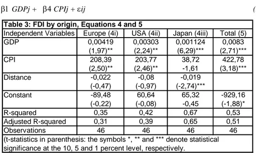
(4iii) as the regression measuring the FDI from Japan. In the following table 3 we can see the results. Which also includes the results of regression (5).
FDIj = β1 GDPj + β4 CPIj + εij (5) Table 3: FDI by origin, Equations 4 and 5
Independent Variables Europe (4i) USA (4ii) Japan (4iii) Total (5) GDP 0,00419 0,00303 0,001124 0,0083 (1,97)** (2,24)** (6,29)*** (2,71)*** CPI 208,39 203,77 38,72 422,78 (2,50)** (2,46)** -1,61 (3,18)*** Distance -0,022 -0,08 -0,019 (-0,47) (-0,97) (-2,74)*** Constant -89,48 60,64 65,32 -929,16 (-0,22) (-0,08) -0,45 (-1,88)* R-squared 0,35 0,42 0,67 0,53 Adjusted R-squared 0,31 0,39 0,65 0,51 Observations 46 46 46 46
(t-statistics in parenthesis: the symbols *, ** and *** denote statistical significance at the 10, 5 and 1 percent level, respectively.
At a first glance at table 3 we can see that once again all the coefficients have the sign we expected, GDP and CPI being positive and distance being negative.
Using this equation instead of (4i) we can see that in all three equations (4ib, 4ii and 4iii) CPI is significant, at a 1 % or 5 % level, confirming what we had seen in section 4,1. We can also see that in all these equations GDP is highly significant. It is interesting to note that the level of R-squared goes from 0,347 in the FDI from EU to 0,67 in the FDI from Japan. This does not necessarily imply that FDI from Japan is more sensitive to either FDI, GDP or distance, but rather that by using this equation we can explain the distribution of FDI more clearly.
Observing the coefficients of CPI, we see that the FDI from USA is the one that is most sensitive to changes in CPI, because of the highest coefficient. Nonetheless this can also have to do with the size of FDI, because the total FDI from Japan is lower than the one from both Europe and USA, so it will naturally have a lower coefficient. Anyway it is interesting to state that FDI from USA is more sensitive to changes in CPI then the FDI from Europe, even though the later has on average higher FDI. Anyway this is also so, because as in equation (4ib) we do not include distance, which in the other cases has a negative effect, the other coefficients have lower values because they do not have to offset this negative effect. We must also state that FDI from Japan has the most significant impact of corruption, at a 1 % confidence level, while in the other cases it is only significant at a 5% confidence level.
Using these equations to calculate the effects of changes of CPI on FDI is tricky. For example, in the equation (4ii), the coefficient of CPI is of 209, meaning that if all things are left the same an increase of the CPI of 1 point (that means a reduction in corruption) would increase FDI from USA to any given country by 209 million dollars. That means that a change in 1 point of the CPI index would have the same effect on a large economy and a small economy, for example China and Paraguay. In spite of this not being a perfect forecaster, or anything close, it is interesting to see that there is a correlation between corruption and FDI.
A last alternative is to measure the total FDI, adding up the FDI from the three regions. In this case the equation is a combination of equations (2) and (4). As we are measuring total FDI to a country, not considering the origin, we can not include the variable of distance. The second difference from equation (2) is that we only use 46 observations, the number of countries we are analysing. So in this way the equation would be:
FDIj = β1 GDPj + β4 CPIj + εij (5)
So in a direct way we see to what extent do GDP and CPI determine the level of total FDI. As expected, once again, both GDP and CPI have positive coefficients and they are statistically significant at a 1% level. It is interesting to see that the R-squared is of 0,517, which shows clearly the relation between these variables. This equation is very useful to confirm our original hypothesis that that corruption does have an effect on FDI, but it does not tell us anything about how it affects in different ways depending on the origin of the investment. Anyway it is useful to include because in this way we can compare with the other equations in table 3.
4.3 Improving
estimations
In this section we shall run a few more regressions in order to measure the effects of corruption on FDI in a more accurate way. We shall run the same regression as before using logarithms and then we shall include dummy variables to see how we can improve our results.
4.3.1 Eliminating zeros and negative investment
In order to increase the accuracy of our estimation an alternative method is to use the logarithms of some of the variables. Logarithm is a monotonic function, so by applying logarithm to some variables it will not change the signs of the coefficients but will change the value of these. This is also very useful to reduce heteroscedasticity. In these tests we want to see the relation between the variables.
One reason to use logarithm is that eliminates values of “zero” and negative FDI. When looking at the total FDI, but even more so when we look at FDI by origin, there are many cases were there is no FDI to one country, mainly in small countries, where maybe there was no investment from some specific region in these years. There are some countries (like Paraguay and Botswana), were on average FDI is actually negative. The reason for this is that maybe the country is taking home dividends, while there is no investment, so there is actually a capital outflow from the developing country to the developed economy. In both these case when we use the log, there is no value, so it is eliminated from the regression. The question is if by eliminating these results we are actually improving the results or not. And more so, if it acceptable from a theoretical background.
In most of the regressions run (2, 4 and 5), if we use log the results of the regression improve. We get higher R-squared and adjusted R-squared, as well as higher level of t-statistics for the variables, the exception is equation (4iii) where the R-squared is reduced if applied logs (this is FDI from Japan). Nonetheless we have to evaluate if it is the most accurate way of calculating the relationship between FDI and CPI. By eliminating the cero and negative values we get a biased sample. The question is if we should use this sample or not. If it is good to measure countries where there is a positive
FDI or better to include all the group of developing countries selected. In the cases where we get a higher R-squared, it will be more helpful to have a general estimation of how sensitive is FDI to CPI. So we can say that given the results we have from equations (1) to (5), where we see that there is a significant relation between CPI and FDI, we can use these equation. So when we analyse the results and reach our conclusions we must keep this into account.
Having explained this, we have modified equation (2), calculating the log of the variables FDI, GDP and distance. In this way we reach equation (6):
LFDIij = β1 LGDPj + β3 LDISTANCEij + β4 CPIj + εij (6)
Where LFDI, LGDP and LDistance represent the logarithms of the respective variables. As we have explained before, “i” represents the country of origin of FDI and “j” represents the host country. We can see the results in table 4. In this case by eliminating all non-strictly positive values, we reduce the sample, from 138 to 104. The R-squared improves from 0,298 to 0,479, showing that as we eliminate many values of FDI that are cero (with different parameters), we can explain more clearly the dependant variable as a function of the independent variable.
In the next step we transformed equation (4) by using the logarithms of the variables GDP, FDI and distance, to create equation (7):
LFDIj = β1 LGDPj + β3 LDISTANCEj + β4 CPIj + C + εij (7)
Here once again, we are comparing the FDI from one region to the developing countries. So we run three regressions, (7i) which shows the log of FDI from Europe, (7ii) which represents the log of FDI from USA and (7iii) which represents the log of FDI from Japan. We can see the results of these regressions in table 4.
Table 4: Log FDI, Equations (6) to (8)
Independent Variables Total (6) Europe (7i) USA (7ii) Japan (7iii) Total (8) Log GDP 1,062 1,008424 1,504533 1,27091 1,045492 (8,289)*** (8,60)*** (8,85)*** (4,728)*** (11,427)*** CPI 0,313 0,328 0,424 0,325 0,387223 (3,522)*** (3,716)*** (3,487)*** (2,16)** (4,440)*** log Distance -0,8399 -0,44 -0,571 -0,942 (-5,03)*** (-3,005)*** (-1,51) (-2,56)** C -0,753 -2,649 -8,771 -3,772 -6,628333 (-0,557) (-1,86)* (-2,66)** (-0,68) (-5,654)*** R-squared 0,479726 0,711459 0,7373 0,593 0,746659 Adjusted R-squared 0,464118 0,689818 0,710124 0,568 0,734301 Observations 104 44 33 27 44 (t-statistics in parenthesis: the symbols *, ** and *** denote statistical significance at the 10, 5 and 1 percent level, respectively.
We can see that in regression (7i) the number of observation included in the regression is reduced only by 2, to 44. This is the region where there is less non strictly positive results, because it is the largest economic area, it has the highest total FDI and in this way has positive investments in most countries analysed, the two exceptions being Paraguay and Botswana. In this case the R-squared increases considerably from 0,35 to 0,686 and all variables are significant at a 1% level. So excluding these results considerably improves the regression.
In regression (7ii), we can see that the observations are reduced by a larger extent, to only 33 when we consider only strictly positive FDI from USA. Once again the R-squared is increased from 0,42 to 0,695 when we apply logarithms. All independent variables are still significant at a 1% level.
Observing the results of running the regression for equation (7iii), which measures the log of FDI from Japan, we can see that the number of observations falls to 27, which are also logical considering that Japan is the smallest economic area and in this way has FDI in fewer amounts of countries, specially the small ones. Anyway, this is the only case were R-squared falls, from 0,67 to 0,585 when we apply logs, which is a contrast to the previous results and to what we expected. It is also interesting to see that the coefficient of the variable CPI is only significant at a 5 % level, compared to the high significance it had in the previous regression. This means that in this case there would be no reason to use this equation instead of the original (4iii).
As we analyse the results of equations (7), we can quickly see that in this case FDI from USA is the one that is most sensitive to changes in corruption, with the highest significance. FDI from Japan and Europe have similar coefficients, but the level of significance is higher from Europe than from Japan.
In this case we can also clearly see that the FDI from Europe is less sensitive to distance than that of Japan or USA, because the negative coefficient is of -0,59 compared to the -1,4 of USA and the -1,14 of Japan. This could mean that for European investments distance is not as much a problem as it is for those coming from Japan or USA. This confirms what we saw in equation (4i), where distance was not even significant.
The last equation we shall look at in this section (8), witch is the equivalent to equation (5) but applying logarithms to the variables:
LFDI = β1 LGDPj + β4 CPIj + C + εij (8)
So this equation measures the total FDI to a country, explained by GDP and CPI. In this case the number of observations decreases by 2 to 44, because once again Botswana and Paraguay are excluded because of their negative FDI. The R-squared improves from 0,517 to 0,747, and that all the explanatory variables are significant at a 1% level. This equation, once again shows the clear relation between the variables studied.
4.4 Implications
From the results we have seen in all regressions, there is a clear relationship between FDI, GDP and corruption. To be able to see the direct relation of corruption and FDI, given a certain level of GDP, we can look at FDI as a percentage of GDP. In the following graph (2) we can see that there is a positive relation between this FDI/GDP and CPI, showing that a higher level of CPI implies a higher rate of FDI.
FDI over GDP and CPI
0 1 2 3 4 5 6 7 8 9 10 0,0% 1,0% 2,0% 3,0% 4,0% 5,0% 6,0% 7,0% 8,0% FDI over GDP (%) CP I Argentina Chile Dominican Republic Uruguay Graph 2
Looking at this graph and the results of the regressions we can clearly say that there is not a perfect relation between the variables analysed. This is so because there are many other variables affecting the decision to invest in another country, and in fact each individual investment considers many factors. Even if you use averages for several years we still have to consider specific situations that affected specific investments that may have changed the results we have.
For example in 1999 Argentina sold the last shares of its public Petrol Company YPF to Repsol, the MNE who’s origin is Spain. So that year FDI from Europe to Argentina jumped from an average of US$ 1716 million (from 1997 to 2004 excluding 1999) to US$ 15098 million. This has a huge implication on the average FDI into Argentina in these eight years we are analysing. If we exclude the 1999, because of this specific reason, the average FDI in Argentina falls from US$ 4621 million to US$ 2688 million, or from 2% of average GDP to 1,2%. Actually if we compare Argentina on the graph 2, we can se that its FDI over GDP is higher to countries with its similar level of corruption, but if we do not count the year 1999 it is closer to them. With this example we just want to illustrate some of the weaknesses of this way of comparing so different countries, but also state that the results could change if we measured other years.
In the specific case of Argentina, if we would try to forecast FDI using any of the regressions, the results would be lower than reality for total FDI or FDI from Europe. For example using equation (5) we can estimate FDI to Argentina to be equal to US$ 2115 million, which is less than half of its actual value. But if we do not take into account the investment into YPF, it is much more accurate. On the other hand we can
would be US$ 639 million when it was actually US$ 644 million. FDI from Japan con be estimated in US$ 89 million but it was in reality only US$ 57,6 million.
Taking this into account that our estimation is not that accurate we can make a base mark estimation of what could be expected if corruption levels fell. Continuing with the example of Argentina, which has a CPI level of 2,95 on average, we shall see what would happen if it reduced its level of corruption to that of its neighbour Chile. Chile had on average a CPI value of 7,12. So if Argentina could increase its level of CPI, reducing its corruption, so that its CPI was 7,12, using our model FDI should increase considerably. From equations (4), we could say that FDI would increase to US$ 2060 million from Europe, to US$ 1551 million from USA and to US$ 283 million from Japan. That is that it could a have FDI at 2% of GDP. Here it is useful to state that the FDI which most changed is the one coming from USA that in theory would jump US$ 872 million per year. In this same example, if we use the equation number (8), which calculates total FDI, using the logs of the variables, the estimated total FDI in Argentina would jump from US$ 1639 million with a CPI of 2,95 to US$ 8233,2 million with a CPI of 7,12. This means that, using this regression, if Argentina could have reduced its corruption level to the one of Chile, it could have FDI of 3,6% of GDP. Chile had FDI inflows of 3,1% of GDP, so this sounds reasonable.
To state another example, we shall look at two small countries in Central America, as Dominican Republic and Uruguay. Using equation (8) we can estimate total FDI into Dominican Republic as being of US$ 131 million, which is close to the real average of US$ 149 million, which is only 0,8% of GDP. CPI in this country is of 3,2, showing a high level of corruption, while GDP is of US$ 18 MM. Uruguay has a GDP of US$ 17,5 MM, a CPI of 4,96 and FDI of US$ 283 million, which represents 1,6% of GDP. Using equation (8), we can estimate that if Dominican Republic could reduce its corruption to that of the level of Uruguay, it could increase its FDI to US$ 260,1 million. This would increase FDI to 1,4% of GDP.
These estimations are made on previous years and the factors moving FDI round the world change. Also it considers applying a general model to all investments, in all countries, which is far from reality. Anyway it is a good way to have a general idea of what effects could a change in corruption levels have on FDI into a country.
5 Conclusions
The objective of this paper was to see if there was any relation between corruption and Foreign Direct Investment, and if there is, if there is any difference depending on the origin of Capital. As we have seen in the results of all regressions, and in the graphs there is a clear negative relation between corruption and FDI. We also saw in graph 1 a clear correlation between CPI and GDP per capita, which could be an interesting area for further research. So our first conclusion is that corruption affects the living standard of the people of a country not only by misallocating productive resources and by its moral effects, but also because it reduces Foreign Direct Investment. As it also has a positive correlation with GDP per capita, we can expect it to be related. We can see that if Dominican Republic would have reduced the level of corruption to that of Uruguay, it could have increased the average FDI per year, from 0,8% of GDP to 1,4%. If Argentina, who has a higher FDI over GDP than expected given its level of corruption, would have reduced its level of corruption to the level of Chile, it could have increased the FDI over GDP from 2% to 3,6%.
Looking at the difference concerning the origin of capital, the results are not strong enough to be able to state that there are significant differences in the effects of corruption on FDI. In spite of this, the model used shows that FDI from USA seems to be the most sensible to corruption in these regressions. We can see this in that in the regressions run, the coefficients are both highly significant and have the highest values. This means that in total the FDI from USA will be more affected by corruption than that coming from Japan and Europe. It is harder to compare there relation between these last two, specially taking into account that on average FDI from Japan accounts for only 16% of that of FDI from Europe, but anyway proportionally FDI from Japan is more sensible to corruption than Europe. To find an explanation for this would be another interesting topic of research. At a first glance, we could suppose that it is related to the level of corruption in the country of origin, but in fact the average CPI rates were of 8,05 for Europe, 7,59 for USA and of 6,61 for Japan. So this is not a good explanation. We can also see that Europe is the region where distance has the lowest effect and it is even insignificant in some cases. So in other words, distance is not such a problem in Europe as it is for USA and Japan.
These implications of the results of this paper are that public policies should aim to reduce corruption levels because they have a negative effect on standard of living. Even though it is not necessary to have written this paper to reach those conclusions, these results add to the number of moral and social arguments why public policy should strongly fight against corruption, because even though there are several cultural differences we strongly defend the position that by reducing incentives to generate corruption, it can be reduced.
References
Ades, A. and Di Tella, R., (1999), Rents, competition and corruption, The American Economic Review, 89, 982-993.
Bardhan, P. (1997), Corruption and development: a review of issues, Journalof Economic Literature, XXXV, 1320-1346.
Braun, M. y Di Tella R. (2000) "Inflation and Corruption". Harvard Business School Working Paper.
Caves, R. 1996. Multinational Enterprise and Economic Analysis. Cambridge, England: Cambridge University Press.
Ciochini, F, Durbin, E; David,T-C, (2003): Does Corruption increase Emerging Market
Bond Spreads, Journal of Economics and business. Sep-Dec, 2003 55 (5-6): 503-28.
Dahlström, T. and Johnson, A. (2007), Bureaucratic Corruption, MNEs and FDI, Jönköping International Business School (JIBS), paper n. 82.
Fisman, Raymond and Roberta Gatti (2002): Decentralization and Corruption:
Evidence Across Countries. Journal of Public Economics, vol. 83, pp. 325-345.
Friedman, E. (2000) “Dodging the Grabbing Hand: The Determinants of Unofficial
Activities in 69 Countries”. Journal of Public Economics, Vol. 76.
Hines, J.R., (1995), Forbidden payment: foreign bribery and American business after
1977, Working paper 5266, NBER.
IMF, The Balance of Payment Manual, International Monetary Fund, September 1993. Johnson, A. (2005), Host Country Effects of Foreign Direct Investment, The Case of Developing and Transition Economics, Jönköping International Business School (JIBS) Dissertation Series, No. 031.
Kaufmann, Daniel, Aart Kraay, and Pablo Zoido-Lobatón, 1999, Governance Matters, World Bank Policy Research Working Paper No. 2196 (Washington: World Bank). Kaufmann, D. (1997) "Corruption: The Facts". World Bank Policy Working Paper. Knack, Stephen, and Philip Keefer, 1995, Institutions and Economic Performance:
Cross- Country Tests Using Alternative Institutional Measures, Economics and Politics,
Vol. 7,No. 3, pp. 207–27.
Mauro, Paolo, 1995, “Corruption and Growth,” Quarterly Journal of Economics, Vol. 110, No. 3, pp. 681–712.
———, 1996, The Effects of Corruption on Growth, Investment, and Government
———, 2004, The persistence of corruption and slow economic growth, IMF Staff Papers Vol. 51, No. 1, 2004 International Monetary Fund.
Markusen, J. 1995. “The Boundaries of Multinational Enterprises and the Theory of
International Trade.” Journal of Economic Perspectives 9: 169-89.
Mody, A. and Wheeler, D., (1992), International investment decisions: The case of
USfirms, Journal of International Economics, 33, 57-76.
North, D. (1990), Institutions, Institutional Change and Economic Performance, Cambirage University Press.
North, D. (1991), Institutions, Journal of Economic Perspectives, 5, 97-112.
Rose-Ackerman, S. (1978): Corruption. A study in political economy. London/New York: Academic Press.
Rose-Ackerman, S. (1996) “The Political Consequences of Corruption. Causes and
Consequences”. World Bank, Note 74.
Smith, Adam (1776), An Inquiry into the Nature and Causes of the Wealth of Nations (New York: Modern Library, 1937 [1776]).
Gert Tinggaard Svendsen (2003): Social Capital, Corruption and Economic Growth:
Eastern and Western Europe. ISSN 1397-4831.
Tanzi, V. y Davoodi, H. (1998) “Corruption, Public Investment and Growth”.
International Monetary Found Working Paper, 97/139.
Wei, S-J, (2000a), How taxing is corruption on internatinoal investors?, The Review of economics and statistics, 82, 1-11.
Wei, S-J, (2000b), Local corruption and global capital flows, Brooking papers on Economic activity, 2000 (2).