UPTEC X 17 007
Examensarbete 30 hp
September 2017
Optimisation of Ad-hoc analysis
of an OLAP cube using SparkSQL
Teknisk- naturvetenskaplig fakultet UTH-enheten Besöksadress: Ångströmlaboratoriet Lägerhyddsvägen 1 Hus 4, Plan 0 Postadress: Box 536 751 21 Uppsala Telefon: 018 – 471 30 03 Telefax: 018 – 471 30 00 Hemsida: http://www.teknat.uu.se/student
Abstract
Optimisation of Ad-hoc analysis of an OLAP cube
using SparkSQL
Milja Aho
An Online Analytical Processing (OLAP) cube is a way to represent a multidimensional database. The multidimensional database often uses a star schema and populates it with the data from a relational database. The purpose of using an OLAP cube is usually to find valuable insights in the data like trends or unexpected data and is therefore often used within Business intelligence (BI). Mondrian is a tool that handles OLAP cubes that uses the query language MultiDimensional eXpressions (MDX) and translates it to SQL queries. Apache Kylin is an engine that can be used with Apache Hadoop to create and query OLAP cubes with an SQL interface. This thesis investigates whether the engine Apache Spark running on a Hadoop cluster is suitable for analysing OLAP cubes and what performance that can be expected. The Star Schema Benchmark (SSB) has been used to provide Ad-Hoc queries and to create a large database containing over 1.2 billion rows. This database was created in a cluster in the Omicron office consisting of five worker nodes and one master node. Queries were then sent to the database using Mondrian integrated into the BI platform Pentaho. Amazon Web Services (AWS) has also been used to create clusters with 3, 6 and 15 slaves to see how the performance scales. Creating a cube in Apache Kylin on the Omicron cluster was also tried, but was not possible due to the cluster running out of memory. The results show that it took between 8.2 to 11.9 minutes to run the MDX queries on the Omicron cluster. On both the Omicron cluster and the AWS cluster, the SQL queries ran faster than the MDX queries. The AWS cluster ran the queries faster than the Omicron cluster, even though fewer nodes were used. It was also noted that the AWS cluster did not scale linearly, neither for the MDX nor the SQL queries.
ISSN: 1401-2138, UPTEC X 17 007 Examinator: Jan Andersson
Ämnesgranskare: Andreas Hellander Handledare: Kenneth Wrife
Populärvetenskaplig sammanfattning
Big Data är ett svårdefinierat begrepp men kan beskrivas som en datamängd som endast kan hanteras med hjälp av ett flertal datorer. Ofta sammanfattas Big Data som data av stor storlek, olika struktur, mycket brus och som inkommer i hög hastighet. Ett sätt att hantera Big Data är genom att bearbeta data parallellt på flera datorer. Det mest använda ramverket för detta är Apache Hadoop och det används genom att implementera det på ett kluster av datorer. Apache Spark, Apache Hive och Apache Kylin är tre komponenter som kan installeras på Hadoop och som kan användas för att analysera data på klustret. Amazon Web Services (AWS) är en molntjänst som kan användas för att skapa ett kluster genom att allokera resurser genom molnet. För att ett företag ska kunna analysera och presentera information om sin data används ofta Business Intelligence(BI)-metoder. Med hjälp av dessa kan information som kan ligga till stöd för olika typer av beslut utvinnas. On-Line Analytical Processing (OLAP) används ofta inom BI eftersom den skapar en multidimensionell datamodell som är optimal att använda vid just analys av data. En OLAP-kub är ett sätt att representera OLAP-data och i denna skapas värden som är av intresse vid en analys. Dessa värden kallas för measures och vanliga exempel är total kostnad, vinst eller försäljning under en viss tid. Mondrian är ett verktyg som hanterar OLAP-kuber och kan implementeras i BI-plattformen Pentaho. Genom detta verktyg kan frågor ställas i frågespråket MultiDimensional eXpressions (MDX) till en OLAP-kub. Mondrian översätter MDX-frågorna till SQL-frågor som sedan skickas till antingen en relationell databas eller till en OLAP-databas. Det finns ett flertal prestandatest som tagits fram för att utvärdera prestandan på databaser. Star schema benchmark (SSB) är ett test som består av en databas och ett flertal Ad-hoc frågor. Databasen har ett så kallat stjärnschemaformat som ofta används av OLAP-kuber.
I detta examensarbete har ett Ad-hoc-frågor i MDX ställts mot en OLAP-kub skapad från SSB-data med över 1,2 miljarder rader. Frågorna har skickades från Pentaho med Mondrian som motor till två typer av kluster: ett stationerat på Omicron Cetis kontor och 3 kluster på AWS av olika storlek. Prestandan har sedan jämförts med prestandan från SQL-frågor som skickats direkt till databasen utan att använda Pentaho. Även skalningen på AWS-klustren analyserades och två försök av att skapa en kub i Apache Kylin på Omicron-klustret gjordes.
Resultaten visade att det tog mellan 8,2 till 11,9 minuter att köra MDX-frågorna på Omicron-klustret och att det gick snabbare att köra SQL-frågorna direkt till databasen. Alla frågor kördes snabbare på samtliga AWS-kluster jämfört med Omicron-klustret, trots att färre noder användes. Varken SQL-frågorna eller MDX-frågorna skalade linjärt på AWS-klustren. Det gick inte att undersöka prestandan av Kylin eftersom Omicron-klustret inte hade tillräckligt med minne för att kunna skapa kuben.
Table of content
Abbreviations ... 1 1. Introduction ... 3 1.1 Purpose ... 4 2. Theory ... 6 2.1 The Hadoop Ecosystem ... 6 2.1.1 HDFS ... 6 2.1.2 YARN ... 6 2.1.3 MapReduce ... 7 2.2 Apache Spark ... 8 2.3 Apache Hive ... 10 2.4 OLAP ... 11 2.4.1 Star schemas and Snowflake schemas ... 11 2.4.2 OLAP Cube ... 12 2.5 Mondrian ... 13 2.6 OLAP on Hadoop ... 14 2.6.1 Apache Kylin ... 14 2.7 SSB benchmark ... 14 2.8 Amazon Web Services ... 15 2.8.1 Amazon EMR ... 16 2.8.1 Amazon Redshift ... 16 2.9 Scaling ... 16 2.10 Previous work ... 17 3. Method ... 19 3.1 Cluster setup ... 19 3.1.1 The Omicron cluster ... 19 3.1.2 The AWS cluster ... 19 3.2 Data ... 20 3.3 Queries ... 21 3.5 Mondrian in Pentaho ... 22 3.6 Running the queries ... 24 3.7 Kylin ... 24 3.8 System benchmark ... 25 4. Results ... 26 4.1 The Omicron Cluster ... 26 4.2 The AWS clusters ... 26 4.2.1 AWS 3 worker nodes ... 27 4.2.2 Aws 6 Worker nodes ... 27 4.2.5 AWS 15 worker nodes ... 28 4.3 Comparing clusters ... 28 4.3.1 Comparing MDX queries ... 29 4.3.2 Comparing SQL queries ... 29 4.4 Scalability ... 30 4.5 Kylin ... 31 4.6 System benchmark ... 32 5. Discussion ... 33 5.1 Omicron cluster vs. AWS clusters ... 335.2 Comparison to previous work ... 33 5.3 AWS instance types ... 34 5.4 Database ... 34 5.5 MDX vs. SQL ... 35 5.6 Scaling ... 35 5.7 Possibilities with Apache Kylin ... 36 5.8 Other OLAP options ... 36 6. Conclusion ... 38 7. References ... 40 Appendix A – MDX queries ... 42 Q1 MDX ... 42 Q2 MDX ... 42 Q3 MDX ... 42 Q4 MDX ... 42 Appendix B – SQL queries ... 42 Q1 SQL ... 42 Q2 SQL ... 43 Q3 SQL ... 43 Q4 SQL ... 43 Appendix C – Omicron Cluster performance ... 44 Appendix D – AWS 3 worker nodes performance ... 44 Appendix E – AWS 6 worker nodes performance ... 44 Appendix F – AWS 15 worker nodes performance ... 45 Appendix G – System Benchmark ... 45
Abbreviations
BI = Business Intelligence CDE = Community Dashboard Editor CPU = Central Processor Unit DAG = Directed Acyclic Graph GB = Gigabyte GiB = Gibibyte HDFS = Hadoop Distributed File System HOLAP = Hybrid OLAP I/O = Input Output JDBC = Java Database Connectivity JNDI = Java Naming and Directory Interface JVM = Java Virtual Machine kB = Kilobyte MB = Megabyte MDX = MultiDimensional eXpressions MOLAP = Multidimensional OLAP OLAP = On-Line Analytical Processing OLTP= On-Line Transaction Processing RAM = Random-access memory RDD = Resilient Distributed Dataset ROLAP = Relational OLAP SSB = Star Schema Benchmark SQL= Structured Query Language YARN = Yet Another Resource Negotiator
1. Introduction
Due to the advances in technology, the amount of data being produced and stored is continuously increasing. However, computers do not have the same increase in performance and are not able to keep up. A way to tackle this problem is to use multiple computers to process data in parallel, instead of relying on the performance of one computer.
The Big Data concept is hard to define, but one definition can be seen as a dataset that only can meet the service level agreements with the use of multiple computers to handle and store the data. This means that the concept depends on the context, making the definition hard to grasp. (Wadkar, S., Siddalingaiah, M. and Venner, J., 2014). The challenge with handling Big Data is not only that it comes in large volume, but also that the data often has different structures, that the pace of the data flow is fast and continuous and because there often is bias and noise in the data. These characteristics can be summarized using the words Volume, Variety, Velocity and Veracity and are called the four V’s of Big Data. Apache Hadoop is the most well known Big Data Technology Platform and is a framework that process large data amounts in parallel. Hadoop consist of an entire ecosystem of components and most of them are open source projects developed under Apache Software Foundations. A few examples of these components or frameworks are Hadoop Distributed File System (HDFS), Map Reduce, Apache Hive, Apache Spark and Apache Kylin (Mazumder, S., 2016). Amazon Web Services is a cloud service that provides Hadoop clusters where users can specify how many resources that are of interest and allocate them through the cloud (Wadkar, S., Siddalingaiah, M. and Venner, J., 2014).
OLAP is an umbrella term for techniques used for analysing databases in real-time. The purpose of the method is usually to find valuable insights in the data, like trends or unexpected data, and is often used within Business intelligence. (Ordonez, C., Chen, Z. and García-García, J., 2011). OLAP uses a data model called multidimensional database that stores aggregated data and creates a simpler representation of the data. This increases the performance of analysing the data
and also makes it easier to maintain and understand. A way to represent the multidimensional database is with the use of OLAP cubes that organises the data into a fact table and multiple dimensions (Cuzzocrea, A., Moussa, R. and Xu, G., 2013). There are different schema types that can be used for multidimensional databases. The star schema is one model that is often used in data warehouse applications (de Albuquerque Filho et al. 2013).
SSB is a benchmark that has been created to measure the performance of data warehouse systems. It also provides generator that allows the user to generate a database in star schema format. The size of the generated database depends on a scaling factor specified by the user (de Albuquerque Filho et al. 2013).
To create and handle an OLAP cube, an open source server called Mondrian can be used. It is integrated into the BI software Pentaho and uses the query language MDX to send queries to a relational database. However, the ad-hoc queries used in BI are usually complex and if the cube is large, it will require a lot of computational power. To increase the performance of the analysis, parallel processing and distributed file systems can be used (Cuzzocrea, A., Moussa, R. and Xu, G., 2013).
1.1 Purpose
This thesis investigates the analysis of ad-hoc queries on OLAP cubes with the use of Apache Spark on a Hadoop cluster. The goal has been to examine whether Spark is suitable for analysis of OLAP cubes and what performance that can be expected. This work will mainly be performed on a cluster consisting of 6 nodes located in the Omicron Ceti office. However, to be able to see how the performance scales with the amount of nodes, clusters of different size created on Amazon Web Services will also be used. The Star Schema Benchmark will be used for generating a database with more than a billion rows.
To handle the cube, Mondrian integrated into Pentaho is to be used. Pentaho also have a Community Dashboard Editor (CDE) (Pentaho, 2017) that will be used for sending MDX queries to Mondrian and to visualise the results. To be able to compare how the BI server affects the performance, the same queries in SQL will also be sent straight to the database on the cluster. Furthermore, Apache Kylin will be examined and tested for OLAP cube analysis.
2. Theory
2.1 The Hadoop Ecosystem
Hadoop is one of the most popular Big Data platforms used today. It is an open-source software that has been developed since 2002 and enables storing and processing of Big Data in a distributed manner (Huang, J., Zhang, X. and Schwan, K., 2015). The fact that it is distributed means that Hadoop is used on multiple nodes in a cluster. Hadoop consists of a number of components where HDFS and MapReduce are the main frameworks used for storing and processing the data (Mazumder, S., 2016). 2.1.1 HDFS
HDFS is a distributed file system and stores the data on several nodes in the cluster. In a large cluster with a large amount of nodes, some nodes will fail every now and then. However, HDFS prevents data being lost by replicating the data on multiple nodes. When a file is uploaded to HDFS, the file is split into blocks of data. This is done using slave components called DataNodes that creates blocks, replicates them and stores them. For HDFS to keep track of what data is stored where, a master component called NameNode is used. There is usually only one NameNode in a Hadoop cluster while there are multiple DataNodes getting instructions from the NameNode (Vohra, Deepak, 2016). 2.1.2 YARN YARN, or MapReduce2, is a framework in the Hadoop ecosystem that handles the distributed processing of the data. Since HDFS and YARN run on the same nodes, the tasks to be run can be scheduled as efficiently as possible. This means that a task is run on the same node where the data to be used is stored (Vohra, Deepak, 2016; Apache Hadoop, Apache Hadoop YARN, 2017). There are two components in YARN that handles the resource allocation and that is the ResourceManager and the NodeManager. All types of applications sent to Hadoop will be allocated a resource for processing. The ResourceManager
running on the master node will schedule this allocation. Each slave node runs a NodeManager that communicates with the ResourceManager and launches containers and monitors their status. A container is a specified amount of resources that is allocated on the cluster in terms of memory and virtual cores. The amount of resources in a container can differ and a NodeManager can have more than one container (Vohra, Deepak, 2016; Apache Hadoop, Apache Hadoop
YARN, 2017).
When an application is sent to Hadoop, the ResourceManager will, via the NodeManager, create a container to run an ApplicationMaster. The ApplicationMaster is a slave daemon and will manage and launch the tasks in the application. It negotiates with the ResourceManager for resources and with the NodeManager for execution of tasks. When the task has finished, the containers are deallocated and can be used for running another task (Vohra, Deepak, 2016; Apache Hadoop, Apache Hadoop YARN, 2017). 2.1.3 MapReduce Map and Reduce task are two types of tasks that can be run on YARN to process data in parallel. The Map interface represents the data as key/value pairs and performs scalar transformations on them. After grouping the result from Map by the different keys, an array of all values associated with each key is created and sent to the Reduce interface. Reduce finally applies some operations on each array and returns the results (Mazumder, S., 2016). An application that counts the amount of words in a text file can be seen as an example to get a better understanding of how the process works. Multiple mappers will go through all the words in the text file and give each word a key-value pair in this way: <<word>, 1>. All the pairs are then grouped so that if a word is found two times in a text, they are put into the same key-value pair. For example, if a word was found 2 times in a text, the key-pair would be: <<word>, 2>. The results from all mappers are then sent to the reducer that sums the values for all the words found in all mappers (Apache Hadoop, 2017, Mapreduce tutorial).
A few examples of components that can run on HDFS with the use of YARN apart from MapReduce are Spark, Flink and Storm. When data comes in streams, in
Real Time or when iterative processing is needed, Map Reduce is not suitable (Mazumder, S., 2016). This is because MapReduce has to read and write from the disk between every job. Instead, Spark that stores the intermediate data in memory can be used (Zaharia, M. et al. 2010).
2.2 Apache Spark
Spark is a Distributed Processing Engine that stores the data sets in-memory, which is called Resilient Distributed Dataset (RDD). This means that the memory of the cluster is used instead of being dependent of the distributed file system. In addition, the distribution of data and the parallelisation of operations are made automatically making Spark both easier to use and faster than MapReduce. However, the fault tolerance and the linear scalability for the two frameworks is the same. Spark core is the heart of Spark and makes the in-memory cluster computing possible. It can be programmed through the RDD API, which comes in multiple languages such as Scala, Java, Python and R (Salloum, S. et al. 2016).
An RDD consists of data that is divided into chunks called partitions. Spark performs a collection of computations on the cluster and then returns the results. These computations are also known as jobs and a Spark application can launch several of them. The job is first split into DAGs, which consists of different stages built of a set of tasks. The tasks are parallel operations and there are two types of them called transformations and actions. Transformation operations define new RDDs and are deterministic and lazily evaluated, which means that they wont be computed before an action operation is called. There are two different types of transformations called narrow and wide transformations. In a narrow transformation, each partition of the child RDD only uses one partition of the parent RDD. Map and filter are two examples of narrow transformations. In a wide transformation on the other hand, several partitions of the child RDD use the same partition of the parent RDD. This means that wide transformations needs data to be shuffled across the cluster which can be expensive since the data needs to be sorted and partioned again. Two examples of wide transformations are join and groupByKey. When data is shuffled in a wide
transformation, a new stage is started since all previous tasks need to be completed before starting the shuffle. Actions are operations that return a result and are therefore found in the end of each job. When the action operation is called, all transformations are first executed, and then the action. Three examples of action operations are count, first and take. As stated above, each job is divided into stages. The amount of tasks in each stage depends on what type of operations that are present in the job. (Salloum, S. et al. 2016). For each partition of the RDD, a task is created and then sent to a worker node (Zaharia, M. et al. 2010).
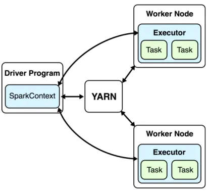
When an application is run in Spark, five entities, namely a cluster manager, a driver program, workers, executors and tasks, are needed. A cluster manager allocates resources over the different applications (Salloum, S. et al. 2016). Spark StandAlone and YARN are two types of cluster managers (Apache Spark, 2017). The driver program access Spark through a connection called SparkContext, which connects the driver program with the cluster. The worker provides the application with CPU, storage and memory and each worker has a JVM process created for the application called the Executor. The smallest units of work that an executor is given are tasks and when the action operation is executed, the results are returned to the driver program (Salloum, S. et al. 2016). An overview of how YARN works with Spark and two worker nodes can be seen in figure 1.
Figure 1 – Shows the overview of a cluster using YARN as a cluster manager and two worker nodes.
Inspired by figure 1 in Apache Spark, Cluster Mode Overview.
SparkSQL is a library that can be built on top of Spark core and is used for processing structured data using SQL. This structured data can for example be stored in a database, parquet files, CSV files or ORC files (Guller, M., 2015).
Hadoop has a similar project called Apache Hive, which transforms SQL queries into Hadoop MapReduce jobs (Lakhe, B., 2016).
2.3 Apache Hive
Apache Hive is a system used for data warehousing in Hadoop. It uses an SQL like language called HiveQL to create databases and send queries that are translated into MapReduce jobs. Hive has a system catalog called Metastore where the metadata of Hive tables are stored in a relational database management system. These Hive tables are similar to tables used in relational databases and can be either internal or external. The difference is that the external table will have data stored in HDFS or some other directory, while the internal table stores the data in the warehouse. This means that the data in an internal table will be lost if the table is dropped, while the data in an external table still will be stored in its original place if the table is dropped (Thusoo, A. et al. 2009). There are two
interfaces to interact with Hive and these are the Command Line Interface (CLI) and HiveServer2. Hiveserver2 has a JDBC client called Beeline that is recommended to be used for connecting to Hive by Hortonworks. (Hortonworks, 2017, Comparing Beeline to Hive CLI). SparkSQL can also be used with Beeline for sending queries to Hive tables but uses a Spark engine instead of a Hive engine. Furthermore, a Spark JDBC/ODBC server can be used for sending queries from for example a BI tool to Spark that then send the queries to the Hive tables (Guller, M., 2015).
2.4 OLAP
In many businesses, On-Line Transaction Processing (OLTP) databases are used for storing information about transactions, employee data and daily operations. OLTP databases are relational databases and usually contain large amounts of tables with complex relations. This makes OLTP databases optimal for storing data and accurately record transactions and similar. However, trying to retrieve and analyse this data will take a lot of time and be computationally expensive. An alternative to OLTP databases is using an Online Analytical Processing (OLAP) database, which extracts data from the OLTP database and is designed for analysing data. The OLAP database is often created from historical data since analysis of a constantly changing database is difficult (Microsoft Developer Network, 2002).2.4.1 Star schemas and Snowflake schemas
The schema structure of an OLAP database differs to the schema used in an OLTP database. There are two types of schemas that are commonly used with OLAP cubes, and these are called star schemas and snowflake schemas. They both consists of multiple dimension tables, a fact table and measure attributes. However, the snowflake schema is a more complex, normalised version of a star schema. The reason for this is because the snowflake schema has a hierarchal relational structure while the star schema has a flat relational structure. This means that in a star schema, the fact table is directly joined to all the dimensions,
while the snowflake schema has dimensions that are only joined to other dimensions (Yaghmaie, M., Bertossi, L. and Ariyan, S., 2012).
In a star schema, the dimension tables contain facts about a certain area of interest. Since time usually is a factor that is taken into consideration during data analysis, it is very common to use a time dimension. Other common dimensions are Product, location and customer (Microsoft Developer Network, 2002). The fact table is the central table that connects the different dimensions with the use of foreign keys. It also contains measure attributes that are created with the use of aggregations such as sum, count and averages. (Ordonez, C., Chen, Z. and García-García, J., 2011). A few examples of common measure attributes are total sales, quantity, discount and revenue. Figure 2 shows an example of how a star schema can be created from a relational schema.
Figure 2 – An example of how a star schema can be created from a relational schema. The schema on the left shows a relational schema and the schema on the right shows a star schema. Inspired by figure 1 and 2 in Microsoft Developer Network, Just What Are Cubes Anyway?.
2.4.2 OLAP Cube
An OLAP cube is a way to represent the data in an OLAP database. Each aggregation function defined in the fact table is calculated for all the facts in each
dimension. For simplicity, consider a star schema containing only one measure attribute: total sales, and three dimensions: Date, Product and Location. The cube will then calculate the total amount of sales for each date, location and product. (Microsoft Developer Network, 2002). There are three different types of OLAP engines called: multidimensional OLAP (MOLAP), relational OLAP (ROLAP) and Hybrid OLAP (HOLAP). MOLAP creates a pre-computed OLAP cube from the data in a database that it sends queries to, while ROLAP uses the data stored in a relational database. A HOLAP also creates a cube but if it is needed, it can send queries straight to the database as well (Kaser, O. and Lemire, D., 2006).
2.5 Mondrian
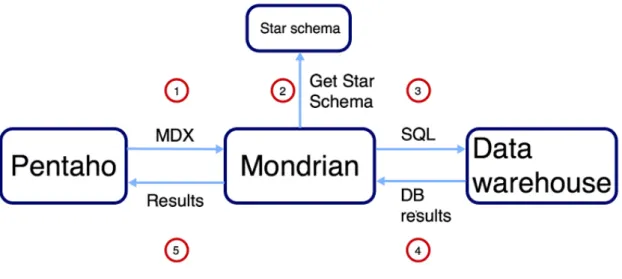
Mondrian is a ROLAP engine used for handling and analysing OLAP cubes. To run the engine, a server is needed and the most popular business analytics server is Pentaho. To be able to make an analysis using Mondrian, a schema defining the OLAP cube is required as well as a JDCB connection to a relational database. Mondrian uses the query language MDX that it transforms into simplified SQL queries that it sends to the database. Figure 3 shows how Mondrian works with Pentaho when a star schema is defined. A user will use the interface of Pentaho to send MDX queries to Mondrian. Mondrian will then use the predefined star schema to either return data from the in-memory cache, or translate the MDX query to SQL queries. The SQL queries are sent to the database and the results are first returned to Mondrian and then returned to Pentaho (Back, D.W., Goodman, N. and Hyde, J., 2013).
Figure 3 – Shows an example of how the connection between Pentaho, Mondrian and the data warehouse works. Inspired by figure 1.9 in Mondrian In Action – Open source business analytics, p.19.
2.6 OLAP on Hadoop
There are several options for creating OLAP cubes in Hadoop without using any BI-tools. A few examples are Apache Lens (Apache Lens, 2016), Druid, Atscale, Kyvos and Apache Kylin (Hortonworks, 2015, OLAP in Hadoop). 2.6.1 Apache Kylin Apache Kylin is an open source tool with an SQL interface that enables analysis of OLAP cubes on Hadoop. Kylin prebuilds MOLAP cubes where the aggregations for all dimensions are pre-computed and stored. This data is stored into Apache HBase along with pre-joins that connect the fact and dimension tables. Apache HBase is a non-relational database that can be run on top of HDFS. If there are queries that cannot be sent to the cube, Kylin will send them to the relational database instead. This makes Kylin a HOLAP engine. Kylin creates the cube from data in a Hive table, and then perform MapReduce jobs to build the cube (Lakhe, B., 2016). In the latest version of Kylin, Spark can be used for creating of the cube. However, the Spark engine is currently only a Beta version (Apache Kylin, 2017. Build Cube with Spark (beta)).2.7 SSB benchmark
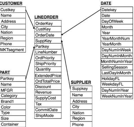
SSB consists of a number of ad-hoc queries that is meant for measuring the performance of a database built of data in star schema format. It is based on the
TPC-H benchmark, but is modified into a star schema consisting of one large fact table called Lineorder and four dimensions called Customer, Part, Date and Supplier. DBGEN is a data generator that generates the 5 tables. By specifying the scaling factor, different sizes of the database can be generated. The 5 tables of the SSB schema can be seen in figure 4 where the arrows demonstrate how the keys are related. There are 6 measures in the Lineorder table and these are: Quanity, ExtendendPrice, Discount, Revenue, Supplycost and Profit. (de Albuquerque Filho et al. 2013).
Figure 4 – The star schema produced by SSB showing the fact table Lineorder in the middle. Inspired by figure 3 in: A Review of Star Schema Benchmark, p. 2.
2.8 Amazon Web Services
Amazon Web Services (AWS) is a cloud services platform that for example can be used for data computation and analysis, networking and the storing of data. There are several cluster platforms that can be used through AWS and these are accessed though the Internet and uses pay-as-you-go pricing. This means that you do not have a contract, but pay for the devices you use at an hourly rate. When using amazon, instances with different amount of CPU, memory and storage can be allocated. More resources will result in a higher hourly rate.
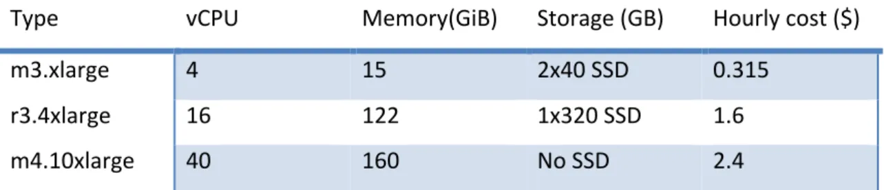
Three examples of different instance types are m3.xlarge, m4.10xlarge and r3.4xlarge and the resources available on these can be seen in table 1.
Table 1 – Shows the available resources on the instance types m3.xlarge, m4.10xlarge and r3.4xlarge on an AWS cluster.
Type vCPU Memory(GiB) Storage (GB) Hourly cost ($)
m3.xlarge 4 15 2x40 SSD 0.315
r3.4xlarge 16 122 1x320 SSD 1.6
m4.10xlarge 40 160 No SSD 2.4
2.8.1 Amazon EMR
Amazon EMR (Elastic map reduce) is a cluster platform that is used for analysis of large data amounts. To enable the processing of this data, frameworks like Apache Hadoop, Apache Spark and Apache Hive is available. The cluster is elastic and this means that the number of provisioned Amazon EC2 instances in each cluster can be scaled dynamically after the users need. During the cluster start up, the user only needs to specify the amount of instances and which frameworks that are of interest. Amazon will then configure the cluster after the users specifications (Amazon Web Services, 2017, Amazon EMR). 2.8.1 Amazon Redshift Amazon Redshift is a data warehouse that supports parallel processing and it stores the data in columns. This means that the columns in a table is divided and distributed into multiple compute nodes. Using a columnar storage means that only the columns used in the query is analysed which can reduce the amount of data that needs to be read from disk and stored in memory (Amazon Web Services, 2017, Performance).
2.9 Scaling
Scaling is a measure of how much time it takes for different amount of processors to execute a program. The time it takes is dependent on the amount
can be seen as a function: 𝑇𝑖𝑚𝑒 𝑝, 𝑥 where p is the amount of processors and x the size of the problem. Measuring the time it takes for one processor compared to multiple processors to execute a problem of a fixed size is called strong scaling. Speedup is a measure of how much a problem is optimised after adding more processors. The speedup can be measured in terms of strong scaling and it can be seen in formula 1. Just as stated above, p is the amount of processors and x the size of the problem. 𝑠𝑝𝑒𝑒𝑑𝑢𝑝 𝑝, 𝑥 =𝑡𝑖𝑚𝑒 1, 𝑥 𝑡𝑖𝑚𝑒 𝑝, 𝑥 (1) The ideal scaling pattern for strong scaling is a linear graph when the numbers of processors are plotted against the speedup. This means that the speedup divided with the amounts of nodes should be close to 1 in ideal scaling and this is more known as linear scaling (Kim, M., 2012).
Another way to estimate how a system scales is to look at the throughput per node. The throughput is the amount of data being processed per time unit. If the throughput is measured in Mb/second, then dividing this with the amount of nodes used for the execution results in Mb/(second*node). If a system has perfect linear scaling, then the throughput per node should be the same for queries ran on different amount of nodes (Schwartz, B., 2015).
However, Gene Amdahl means that this perfect scaling cannot always be expected. He proposed a law called Amdahls Law that states that a problem has two parts: one that is optimisable and one that is non-optimisable. This means that he claims that there is a fraction of a problem that wont get a decreased execution time, regardless of the amount of processors involved (Kim, M., 2012).
2.10 Previous work
The SSB benchmark has been used and studied with Spark before. Benedikt Kämpgen and Andreas Harth that translated the SSB benchmark queries from SQL to MDX in their article called No size Fits All is one example. They compared the performance of the SSB benchmark using both SQL and MDX with Mondrian
just like in this thesis. The results that they obtained for each query can be seen in table 2. Table 2 – Shows how the results that Benedikt Kämpgen and Andreas Harth obtained in the article No size Fits All. Language Q1 Q2 Q3 Q4 MDX 14.7s 14.5s 5.1s 4.8s SQL 15.47s 15.4s 5.3s 5.0s The database was in their case stored in a MySQL database and the database only consisted of around 6 million rows. A cluster was not used either, but a computer with a CPU of 16 cores and 128GB RAM.
Another example is The Business Intelligence of Hadoop Benchmark that was released in 2016. They also used the SSB benchmark to measure the performance of Spark 2.0. However, they only measured the performance of the original SQL queries and they also used a larger database consisting of more than 6 billion rows. The results can be seen in table 3. Table 3 – Shows how the results that AtScale presented in their article The Business Intelligence of Hadoop Benchmark when measuring the performance of SQL on SSB. Language Q1 Q2 Q3 Q4 SQL 11.0s 10.6s 30.3s 13.2s
The cluster used consisted of 1 master node, 1 gateway node and 10 worker nodes. Furthermore, each node had 128G RAM, 32 CPU cores along with 2x512Mb SSD. In Spark, 70 workers were used with 16 GB memory and 4 cores each. The data format used was Parquet.
3. Method
A number of implementations were needed in order to be able to estimate the performance of ad-hoc queries on OLAP cubes with Spark. This included a cluster with the right configurations, data to populate the database with, a database on the cluster, an engine to handle the OLAP cube, an interface where queries are specified and a schema defining the OLAP cube. Furthermore, Kylin was implemented into Hadoop in order to try to create a ROLAP cube. Since different hardware has been used on the different clusters, a system benchmark was run on the master node of the clusters.
3.1 Cluster setup
Two different types of clusters were used to perform the work: a cluster located in the Omicron Ceti office and offices created on AWS. The purpose of using the AWS cluster was to be able to create clusters of different size. This is because by measuring the performance on different sized clusters, it is possible to estimate the scaling of the performance.3.1.1 The Omicron cluster
The cluster in the Omicron Ceti office consists of 6 nodes where 1 node is a master and the other 5 are worker nodes. The RAM in each data node is 16 GB and 4 virtual CPU cores. Hadoop version 2.5.3.0 and Hive version 1.2.1000 have been used. The Spark version used on the cluster was version 2.0.0. However, when running and Kylin, Spark with version 1.6.3 was used as the engine. The version of Kylin was 2.0.0.
3.1.2 The AWS cluster
The clusters created on the AWS cloud consisted of 3 different sizes. The clusters all had one master node but had a different amount of name nodes. The numbers of name nodes in the three clusters were 3, 6 and 15. Every node was of size m3.xlarge meaning that the virtual CPU had 4 cores and that the RAM was 15 GB. The software implemented on the clusters was Hadoop version 2.7.3, Hive version 2.1.0 and Spark version 2.0.2.
3.2 Data
There are several benchmarks that previously have been used for testing the performance of data warehouses such as TPC-H. However, the database used in the TPC-H benchmark is not in star schema format, and is not suitable for this kind of analysis where OLAP cubes are used. Therefore, the Star Schema benchmark (SSB), which has been developed from the TPC-H benchmark, was used instead.
It was decided that a database of at least 1 billion rows was needed to be able to call the task a Big Data problem. Therefore, the scaling factor 200 was used to create the database with SSB’s data generator DBGEN. This resulted in a fact table of more than 1.2 billion rows. The generator returns 5 text files where each file contains the information about a specific table. The size and the amount of rows of each table can be seen in table 4. Table 4 – Shows the file size and the amount of rows in each of the tables created when using scaling factor 200
Table File size Rows
Lineorder 119 GB 1 200 018 603 Customer 554 MB 6 000 000 Part 133 MB 1 600 000 Supplier 33 MB 400000 Dates 225 kB 2556 Data files saved in parquet format will run better with Spark SQL than normal text files. This is because parquet files use a compressed columnar storage format (Ousterhout, K. et al. 2015). Therefore, the text files were also converted into parquet files and this took about 6 hours on the Omicron cluster. When running the SQL queries on the database created from the parquet file however, the queries took about 2-3 times longer to run. Furthermore, since the AWS cluster cost money every hour a cluster is up and running, it would be more expensive to create parquet files from the generated text files. It was therefore decided to use the original text files.
A problem with DBGEN is that it creates the data files on the master node. This means that the master node needs to have storage for 120 GB, which was not the case on the master node on the AWS cluster. Therefore, a DBGEN that created the tables straight into HDFS using MapReduce was used1. This created 5 folders,
one for each table, with all the output data divided into smaller part files on HDFS. All files were by default compressed, which causes problems when trying to create a database from the data. The settings were therefore changed in the java code so that uncompressed text files were saved on HDFS instead.
3.3 Queries
The SSB benchmark queries consist of 13 queries that can be divided into four blocks with different selectivity. All queries are originally in SQL syntax, but have been translated into MDX queries by Benedikt Kämpgen and Andreas Harth in 20132.
The queries were first run against the database on the local cluster and the results were inspected. Unfortunately, Pentaho could not handle casting values as “numeric” and a syntax error was therefore returned whenever this operation was used. There was also one MDX query that started “WITH MEMBER” instead of “SELECT” which is usually used and also returned a syntax error. Two queries did not return any results neither when running it through Pentaho using MDX, nor when using SQL directly on the database using Beeline. This means that only four of the 13 MDX queries could be handled by Pentaho and returned results. Luckily, the queries working belonged to the blocks that used medium and high dataset complexity and volume. All four working queries can be found in both SQL and MDX syntax in Appendix A and B. In the SSB
1 https://github.com/electrum/ssb-dbgen
2 http://people.aifb.kit.edu/bka/ssb-benchmark/
benchmark, these queries are called Q2.2, Q2.3, Q4.2 and Q4.3, but are for simplicity called Q1, Q2, Q3 and Q4 here.
Query Q1 and Q2 make three JOIN operations, two GROUP BY operations and two FILTER operations. However, Q2 is more selective than Q1. Query Q3 and Q4 on the other hand makes four JOIN operations, three GROUP BY operations and three FILTERS and Q4 is more selective than Q3 (The business intelligence on hadoop benchmark, 2016).
A database consisting of Hive tables was created with the use of Beeline. By specifying which port that Beeline should connect to, Hive or Spark could be used as the engine. Since it took many hours to produce the tables with DBGEN, external tables were chosen so that the data would not be dropped if a table were. With Beeline, queries were easily sent to the database with SQL like syntax.
3.5 Mondrian in Pentaho
It was already decided that the OLAP engine Mondrian was to be used for creating and handling the OLAP cube. However, Mondrian cannot run alone and needs a server and in this case, the server Tomcat was used. Tomcat can be either run in standalone mode, or integrated into other webservers. Tomcat standalone was first used with Pivot4j as the Java API. However, the results from the queries came in too large sizes and could therefore not be represented by Pivot4j. Therefore, Tomcat integrated into Pentaho was used. The Pentaho server was running from my personal laptop.
To be able to send queries from Pentaho to a cluster, a JDBC connection is needed. Since the idea was to send queries to SparkSQL, a Spark JDBC connection needed to be used. However, this connection was not working in Pentaho. To get the connection to work, Pentaho’s data integration tool called Kettle was used since it is simpler than Pentahos platform for analysis. A Spark JDBC jar file, 14
other jar files and a licence file were downloaded from Simba3. However, for the
connection to be successful, only four of these 14 jars were to be included in the setup. These four jars were: hive_service.jar, httpclient-4.13.jar, libthrift-0.9.0.jar and the TCLIServiceClient.jar. The Spark JDBC jar, the licence file and the four jar files specified above were put into two lib folders in Pentaho45. Since there is a
charge to use the full version of Simba’s JDBC connectors, a trial version was used. The difference was that the licence file was only available for a month. Therefore, a new licence was simply downloaded when the licence ran out and put in the two lib folders. Another configuration needed to connect to the cluster was to set active.hadoop.configuration = hdp24 in the plugin.properties file6.
After making these configurations, the IP address of the cluster was specified along with the connection port and the name of the database created on the cluster. The default port for Spark is 10015. When the connection was successful, the JDBC connection becomes available under data sources. For Mondrian to be able to create an OLAP cube, an OLAP schema needs to be specified. This is done using an XML metadata file that specifies the attributes in the fact table and the dimensions, the primary keys and the measures. However, it was not possible to upload this file straight into Pentaho. Instead, Pentaho’s Mondrian Schema Workbench was used to publish the cube into Pentaho. Benedikt Kämpgen and Andreas Harth present an XML schema2 that they have
used to create an SSB OLAP schema. This XML file was used, but modified using Schema Workbench so that it corresponded completely to the SSB database on the cluster. After the schema was correctly specified, it was published to Pentaho. When published, it appeared under data sources in Pentaho. 3 http://www.simba.com/product/spark-drivers-with-sql-connector/ 4 pentaho-server/pentaho-solutions/system/kettle/plugins/pentaho-big-data-plugin/hadoop-configurations/hdp24/lib/ 5 pentaho-server/tomcat/webapps/pentaho/WEB-INF/lib/ 6 pentaho-server/pentaho-solutions/system/kettle/plugins/pentaho-big-data-plugin/plugin.properties
Since Pivot4j could not represent the amount of data returned by the queries, the Pentaho tool “Analysis Report” was to be used instead. However, this feature was only available on the enterprise edition of Pentaho, and the community edition was the one running on my laptop. Luckliy, Omicron had Pentaho running in enterprise edition on an instance on AWS. The MDX queries were run on the Analysis Report tool, but unfortunately, it could not represent the resulting data either.
CDE was the tool that finally managed to return and represent the data form the MDX queries. When using CDE, a datasource type needs to be selected, and here, “mdx over mondrianJndi” was used. Since a JDBC connection already has been created, only a JNDI connection is needed where the JDBC connection is selected as source. A Mondrian schema also needs to be specified, and the one published through Schema workbench was therefore used. The component chosen to represent the data was Table. This means that the results from the queries were represented in a table.
3.6 Running the queries
Each query was run 10 times in order to provide a consistent result. The SQL queries were sent to the database using Beeline. The MDX queries were sent to the database through Pentaho’s CDE. In order to prevent Pentaho from caching, the server was restarted between each run. Furthermore, the System Settings, Reporting Metadata, Global Variables, Mondrian Schema Cache, Reporting Data Cache and the CDA Cache were also refreshed between each run. The time it took for each query to run was observed from the Spark Application master. There, each job being executed was shown along with the time it took to run them.
3.7 Kylin
Apache Kylin version 2.0 was downloaded and installed on the master node on the Omicron Cluster. Two different sized cubes were then created in Kylin with all the dimensions, joins, and measures present in the database. The large cube was to be created from the SSB database used in the benchmarking. A smallerlatest version of Kylin, the user can build the cube using Spark as the engine. This feature is at current time only in Beta version.
3.8 System benchmark
In order to compare performance the two cluster types properly and find possible bottlenecks, a system benchmark was run. The benchmark is called Sysbench and the performance of the CPU, reading and writing to RAM and Input/Output (I/O) reading and writing was measured. The commandos used for the benchmark can be seen in Appendix G.
4. Results
Each query in SQL and MDX was run 10 times and the results from each run can be observed in Appendix C, D, E and F. In the following sections, only the average time it took to run the 10 runs is shown. It was noted that for each query, regardless of language, the last partition took much longer to run than the other partitions.4.1 The Omicron Cluster
The time it took for the cluster when running the MDX queries from Pentaho and the SQL queries from Beeline towards the SSB database on the cluster placed in the Omicron Ceti office can be observed in table 5.
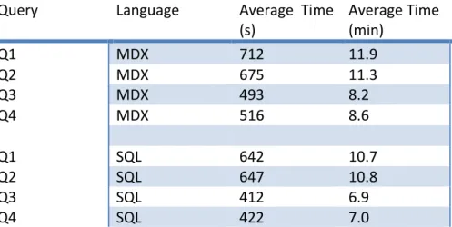
Table 5 – Shows the time it took to run the four queries in MDX and SQL on the Omicron cluster
Query Language Average Time
(s) Average Time (min) Q1 MDX 712 11.9 Q2 MDX 675 11.3 Q3 MDX 493 8.2 Q4 MDX 516 8.6 Q1 SQL 642 10.7 Q2 SQL 647 10.8 Q3 SQL 412 6.9 Q4 SQL 422 7.0 It can be noted that the SQL queries run a bit faster than the MDX queries. How much faster the SQL queries ran can be seen in table 6.
Table 6 – Shows the time difference in seconds between queries in MDX and SQL on the Omicron cluster.
Q1 Q2 Q3 Q4
Time difference
(s) 70 28 81 94
4.2 The AWS clusters
Three different sized AWS clusters were run. The first one had 3 worker nodes, the second one 6 worker nodes and the final one 15 worker nodes.
4.2.1 AWS 3 worker nodes
The average time it took to run the MDX and SQL queries on the AWS cluster with 3 worker nodes are shown in table 7.
Table 7 – Shows the time it took to run the four queries in MDX and SQL on the AWS cluster with 3 worker nodes
Query Language Average Time
(s) Average Time (min)
Q1 MDX 499 8.3 Q2 MDX 491 8.2 Q3 MDX 396 6.6 Q4 MDX 418 7.0 Q1 SQL 437 7.3 Q2 SQL 434 7.2 Q3 SQL 362 6.0 Q4 SQL 363 6.0
The SQL queries ran faster than the MDX queries and how much faster can be seen in table 8. Table 8 – Shows the time difference in seconds between queries in MDX and SQL on the AWS cluster with 3 worker nodes. Q1 Q2 Q3 Q4 Time difference (s) 62 57 34 55
4.2.2 Aws 6 Worker nodes
In table 9, the average time it took to run the MDX and SQL queries on the AWS cluster with 6 worker nodes can be observed.
Table 9 – Shows the time it took to run the four queries in MDX and SQL on the AWS cluster with 6 worker nodes.
Query Language Average Time
(s) Average time (min)
Q1 MDX 299 5.0 Q2 MDX 305 5.1 Q3 MDX 260 4.3 Q4 MDX 265 4.4 Q1 SQL 233 3.9 Q2 SQL 248 4.1 Q3 SQL 198 3.3 Q4 SQL 209 3.5
Yet again, the SQL queries run faster than the MDX cluster. How much faster can be seen in table 10. Table 10 – Shows the time difference in seconds between queries in MDX and SQL on the AWS cluster with 6 worker nodes. Q1 Q2 Q3 Q4 Time difference (s) 66 57 64 56
4.2.5 AWS 15 worker nodes
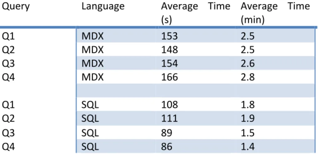
The average time it took to run the MDX and SQL queries on the AWS cluster with 15 worker nodes can be seen in table 11.
Table 11– Shows the time it took to run the four queries in MDX and SQL on the AWS cluster with 15 worker nodes
Query Language Average Time
(s) Average Time (min)
Q1 MDX 153 2.5 Q2 MDX 148 2.5 Q3 MDX 154 2.6 Q4 MDX 166 2.8 Q1 SQL 108 1.8 Q2 SQL 111 1.9 Q3 SQL 89 1.5 Q4 SQL 86 1.4 In table 12, the difference in time it took to run the queries in SQL and MDX can be seen. It can be observed that the SQL queries ran faster than the MDX queries. Table 12– Shows the time difference in seconds between queries in MDX and SQL on the AWS cluster with 15 worker nodes. Q1 Q2 Q3 Q4 Time difference (s) 45 37 65 80
4.3 Comparing clusters
Figure 5 shows a histogram over how long it took to run all queries on all 4 clusters. The blue columns show the time it took to run the queries on the Omicron cluster. The red, green and purple columns shows the time it took to run the queries on the AWS cluster with 3, 6 and 15 worker nodes.
Figure 5 – Shows the time it took to run all the queries on all different clusters. 4.3.1 Comparing MDX queries The plot seen in figure 6 shows the time it took to run the MDX queries on all 4 clusters. Figure 6 – Shows the time it took to run the four MDX queries on the 4 different clusters. 4.3.2 Comparing SQL queries In plot in figure 7 shows the time it took to run the SQL queries on the 4 different clusters. 0 100 200 300 400 500 600 700 800 Q1 Q2 Q3 Q4 T Im e (s) Queries
Comparison of all queries
Omicron MDX Omicron SQL AWS 3 Workers MDX AWS 3 Workers SQL AWS 6 Workers MDX AWS 6 Workers SQL AWS 15 Workers MDX AWS 15 Workers SQL 0 100 200 300 400 500 600 700 800 Q1 Q2 Q3 Q4 T im e (s) QueriesMDX queries performance
Omicron Cluster AWS 3 Workers AWS 6 Workers AWS 15 Workers
Figure 7 – Shows the time it took to run the SQL queries on the different clusters.
4.4 Scalability
The master node on the AWS cluster did not have enough storage to store the SSB database of 120 GB. Furthermore, the smallest amount of worker nodes required to produce the SSB database straight on to HDFS using MapReduce jobs was 3 nodes. Therefore, it was not possible to measure the performance of only using one worker node. This means that it was not possible use equation 1 for measuring the scaling.
Instead, the throughput was estimated. The total size of the dataset was 119 720.225 Mb. This means that the throughput is this number divided by the time it took to run each query. The throughput for each query on the different sized clusters was then divided with the amount of nodes used. The results can be seen in table 13 for queries run in MDX and in table 14 for queries ran in SQL. 0 100 200 300 400 500 600 700 Q1 Q2 Q3 Q4 T im e (s) Queries
SQL queries performance
Omicron Cluster AWS 3 Workers AWS 6 Workers AWS 15 WorkersTable 13 – Shows how the AWS cluster scales on the MDX queries when using 3, 6 and 15 nodes.
#Nodes Query Throughput (Mb/s) Throughput/#Node
(Mb/(s*node)) 3 Q1 239.9 80.0 6 Q1 400.4 66.7 15 Q1 782.5 52.2 3 Q2 243.8 81.3 6 Q2 392.5 65.4 15 Q2 808.9 53.9 3 Q3 302.3 100.8 6 Q3 460.5 76.8 15 Q3 777.4 51.8 3 Q4 286.4 95.5 6 Q4 451.8 75.3 15 Q4 721.2 48 Table 14 – Shows how the AWS cluster scales on the SQL queries when using 3, 6 and 15 nodes.
#Nodes Query Throughput (Mb/s) Throughput/#Node
(Mb/(s*node)) 3 Q1 274.0 91.3 6 Q1 513.8 85.6 15 Q1 1108.5 73.9 3 Q2 275.9 92.0 6 Q2 482.7 80.5 15 Q2 1078.6 71.9 3 Q3 330.7 110.2 6 Q3 604.6 100.8 15 Q3 1345.2 89.68 3 Q4 329.8 108.9 6 Q4 572.8 95.5 15 Q4 1392.1 92.8
4.5 Kylin
Unfortunately, it was not possible to run queries on Apache Kylin running on the Omicron cluster. This was because Kylin failed during the creation of the MOLAP cube. The cube to be created from the large database failed during stage 3 out ofthe 11 stages. This stage extracts the distinct columns in the fact table and failed because all the memory was used. The cube to be created from the smaller database managed to run to stage 7 which built the cube with Spark. This also failed due to the system being out of memory.
4.6 System benchmark
The values obtained in the benchmark where the CPU, RAM read, RAM write, I/O write and I/O for the master nodes on two clusters can be seen in figure 8.Figure 8 – Shows the performance of CPU, RAM read, RAM write, I/O write and I/O Read on the master nodes of the two clusters. The values are normalised to percentage in order to compare performance. 0% 20% 40% 60% 80% 100% 120% CPU [20k/s] RAM read [MB/s] RAM write [MB/s] IO write [MB/s] IO READ [MB/s]
System benchmark
AWS Omicron Cluster5. Discussion
5.1 Omicron cluster vs. AWS clusters
How the performance of the clusters differs can easily be seen in figure 6. Here, it can be seen that the Omicron cluster performs worse than any of the AWS clusters, even if fewer worker nodes are used. This can also be observed in figure 7 and 8. The reason for this is either due to bandwidth between the nodes or hardware. The performance of the system benchmark seen in figure 9 shows that the CPU and the RAM is faster on the Omicron cluster. The I/O read on the Omicron cluster is also a lot faster than the AWS cluster. However, this is probably because the Omicron cluster read from RAM instead of from disk since it is not likely that it reads at almost 4 GB/s from disk. The I/O read value from the Omicron cluster should therefore not be taken into consideration. It can be noticed that the I/O write on the AWS cluster is much faster than the Omicron cluster. It is therefore very likely that it is the writing and reading that is the bottleneck for the Omicron cluster. Ousterhout, K. et al. in 2015, showed that when running Spark SQL queries on compressed data, like in parquet, the CPU was the bottleneck. However, when running the same queries on uncompressed data like in this thesis, the queries became I/O bound. This further implies that it could be the I/O that is the bottleneck in this case. The bandwidth between the nodes was not measured, but it could be that this is faster for the AWS cluster as well since they for example could be launched on the same machine.
5.2 Comparison to previous work
In section 2.10, discussing previous work, it can be seen that they have obtained much better performance on the queries than the ones obtained here. It becomes very obvious when comparing table 2 and 3 with table 5, 7, 9 and 11. However, the setup used in this thesis was not same. For example, in the article No size fits All, MDX queries were also sent through Mondrian, but a smaller database of around 6 million rows, stored in MySQL, was used. The computer used also had 128 GB RAM and 16 cores. In the article The Business Intelligence on Hadoop Benchmark that was also mentioned in section 2.10, a larger database consisting of more than 6 billion rows was used. Still, a better performance was obtained. In
this case, only SQL queries were used and the database was stored in MySQL. The cluster was also different. Firstly, the cluster had a gateway node and 10 worker nodes. Secondly, each worker node also had 128GB RAM and 32 CPU cores. This can be compared to the 15GB RAM and 4 CPU cores the available on each node in the AWS cluster used in this thesis showing that a lot more RAM and CPU cores are used.
The reason why Spark performs well is because it saves data into memory. However, when a dataset is too large, Spark will save the data back to disk and this is a large bottleneck of Spark. It is therefore likely that this has happened in this benchmark since the nodes had quite low amounts of RAM compared to what others have used.
5.3 AWS instance types
Table 1 shows the hourly cost for three different instance types on AWS. There are no instances on AWS with 128 GB RAM and 32 CPU cores as used in the previous studies discussed above. However, m4.10xlarge and r3.4xlarge are the instances with the most similar amount of resources. It can be noted that the hourly rate is almost 5 and 8 times more expensive for m4.10xlarge and r3.4xlarge compared to the m3.xlarge instance that has been used in this project. An hour of using a cluster of in total 12 nodes would cost 3.78$ for type m3.xlarge, 19.2$ for type r3.4xlarge and 28.8$ for type m4.10xlarge.
5.4 Database
In this thesis, the database was created in Hive Metastore in Hive tables. This was used since Pentaho/Mondrian needs a JDBC connection to a database in order to use Spark SQL and there is no other feature for this in Hadoop. The data in the previous work was stored in a MySQL database and this could possibly increase the performance of Spark. However, a connection from Pentaho to a database is either through a MySQL JDBC connection or a Spark JDBC connection. This means that it becomes impossible to send SparkSQL queries to a MySQL database through Pentaho. Before running the SQL queries through Beeline to
cluster. The data was stored into parquet files and Hive tables were not used. The performance was not registered, but it took around a minute to run the SQL queries. This implies that using Hive tables is not optimal when using Spark.
5.5 MDX vs. SQL
In all four clusters, the SQL queries ran faster than the MDX queries and this can easily be seen in figure 5. By looking at table 6, 8, 10, and 12, one can observe just how much faster the SQL queries ran. It varied between 28 seconds and 94 seconds difference. However, most of the queries were around 60 seconds, or 1 minute faster. In table 2, it can be observed that MDX queries ran a tiny bit faster than the SQL queries in the article No size fits All. This implies that it is not Mondrian or badly translated MDX queries slowing down the performance. It could therefore be because of the Simba Spark JDBC driver being slow, because Pentaho slows down the progress or because the cube schema defined in XML was not optimised for the data.5.6 Scaling
In ideal linear scaling, the throughput per node should have been the same for all sized clusters running the same query. This means that the throughput/#nodes in the MDX queries seen in table 11 should have been around 80 Mb/(s*node) for query Q1, 81 Mb/(s*node) for query Q2, 100 Mb/(s*node) for query Q3 and 95 Mb/(s*node) for query Q4. Furthermore, the throughput/#nodes in the SQL queries seen in table 12 should have been around 91 Mb/(s*node) for query Q1, 92 Mb/(s*node) for query Q2, 110 Mb/(s*node) for query Q3 and 108 Mb/(s*node) for query Q4. By looking at table 11 and 12, it becomes obvious that this is not the case, which means that neither of the systems scale linearly. However, the SQL queries scale better than the MDX queries since the drop in throughput is not as high and is closer to the ideal value. The reason why none of the queries scaled linearly could be due to what is stated in Amdahls law. It proposes that there is a part of each application that cannot be parallelized. In that case, it could be that there is a large part of the queries that cannot be parallelized, causing a very non-linear scaling. As stated in section 2.2,wide transformations such as Join and GroupBy operations are computationally expensive and require data from different partitions to be shuffled across the cluster. These shuffles require that all tasks are completed before the next stage can start. If the partitions have different amount of data stored on them, some of the tasks will run faster than others and stay on hold until the last task is done. This scenario prevents parallelism and could be a possible answer to why the scaling has been so bad. If this is the case, then a possible solution to this problem could be to change the amount partitions and their size. It is also possible to change the amount of partitions used specifically in shuffles. It is likely that uneven partitions are causing problems since a large fact table is to be joined with smaller dimension tables. Another possible solution for solving this could be to use broadcast joins. This type of join is only useful when a small table is to be joined with a large one since it stores the data of the small table in memory on all the nodes. Not only could this prevent a shuffling stage, but it could also improve the speed of the join since the large data amount does not have to be moved across the cluster.
5.7 Possibilities with Apache Kylin
As previously stated, it was not possible to run any queries with Apache Kylin due to failure during the cube building stage. The reason for failure was because the size of the cube was too large and the system ran out of memory. This was not unexpected since such a large cube had to be created in this benchmark and this is the problem with using MOLAP cubes. However, if a smaller cube was to be used in a future application, I would recommend trying to use Kylin for sending MDX queries to a database. Then, it would not matter if the data is saved in a Hive table since all the data is available in the cube. It can take a long time to create a MOLAP cube, but when it is initiated, the queries will run fast. Kylin is also very user friendly and monitors a lot of the performed work.
5.8 Other OLAP options
Building OLAP cubes in Hadoop is still a new area that has not been fully
developed nor tested. Apart from Apache Kylin, there are several other OLAP-on-promise the world, but it is very hard to find any articles that prove that what they say is true. Apache Kylin is the most documented technology and it is therefore easy to say that it seems to be the most promising one at the moment. Using Amazon Redshift as a data warehouse instead of storing the data in Hadoop could be another option. Redshift uses a columnar storage, which can be benefical to use since only the columns needed are used. It should not be hard to set up a JDBC connection from Pentaho to Redshift. However, I cannot find any documentation or articles of the performance when using Redshift for large OLAP cubes.
6. Conclusion
The queries running on the Omicron cluster ran slower than all queries running on the AWS cluster, regardless of their size. In this case, the bottleneck for the Omicron cluster was probably due to disk I/O writing and reading. Compared to previous work, worse performance was obtained. This was probably because a much more RAM and CPU was used in those cases. Since Spark spills data that is too large to save in memory to disk, a large amount of RAM is probably needed in order to obtain good performance when benchmarking such a large database. Another possible reason for why worse results were obtained could have been because the data was stored in Hive tables. The problem with Pentaho is that data stored in a MySQL database cannot be queried using Spark SQL from Pentaho. It took between 8.2 to 11.9 minutes to run the MDX queries on the Omicron cluster and the SQL queries ran between 28 to 94 seconds faster. In general for all queries, it took about 1 minute faster to run the SQL queries. The reason for this could be either due to the JDBC driver being slow, because using Pentaho slows the process down or because a non-optimal cube schema was used. The scaling of the AWS cluster was not linear and the reason for this could be because there was a large part of the application that could not be parallelized. The reason for this could be because the data was not partitioned evenly and this could be further investigated. Using broadcast joins could help reducing the uneven partitioning when using star schemas with a large fact table and smaller dimension tables.A possible solution for increasing the performance could have been to use Apache Kylin. Not only would performance probably increase since it uses MOLAP cubes, but sending queries to Hive tables and going through a BI tool such as Pentaho could be avoided. It is also user-friendlier and there is no need to specify a cube schema in XML. Unfortunately, it was not possible to create a cube on the Omicron cluster because it ran out of memory. If a smaller cube was
to be created in a future application however, it is possible that it could have worked. There is at the moment not much documented information about the performance of OLAP cubes on clusters. Kylin seems to be the most documented technology, but there are others such as Atscale, Kyvos and Apache Lens. Another option could be to use Amazon Redshift as a data warehouse and store the data there instead of on Hadoop.