Increasing Rule Extraction Accuracy by Post-processing GP Trees

Abstract—Genetic programming (GP), is a very general and efficient technique, often capable of outperforming more specialized techniques on a variety of tasks. In this paper, we suggest a straightforward novel algorithm for post-processing of GP classification trees. The algorithm iteratively, one node at a time, searches for possible modifications that would result in higher accuracy. More specifically, the algorithm for each split evaluates every possible constant value and chooses the best. With this design, the post-processing algorithm can only increase training accuracy, never decrease it. In this study, we apply the suggested algorithm to GP trees, extracted from neural network ensembles. Experimentation, using 22 UCI datasets, shows that the post-processing results in higher test set accuracies on a large majority of datasets. As a matter of fact, for two setups of three evaluated, the increase in accuracy is statistically significant.

I. INTRODUCTION

Most high-accuracy techniques for predictive classification produce opaque models like artificial neural networks (ANNs), ensembles or support vector machines. Opaque predictive models make it impossible for decision-makers to follow and understand the logic behind a prediction, which, in some domains, must be deemed unacceptable. When models need to be interpretable (or even comprehensible) accuracy is often sacrificed by using simpler but transparent models; most typically decision trees. This tradeoff between predictive performance and interpretability is normally called the accuracy vs. comprehensibility tradeoff. With this tradeoff in mind, several researchers have suggested rule extraction algorithms, where opaque models are transformed into comprehensible models, keeping an acceptable accuracy. Most significant, are the many rule extraction algorithms used to extract symbolic rules from trained neural networks; e.g. RX [1] and TREPAN [2]. Several papers have discussed key demands on reliable rule extraction methods; see e.g. [3] or [4]. The most common criteria are: accuracy (the ability of extracted representations to make accurate predictions on previously unseen data), comprehensibility (the extent to which extracted representations are humanly comprehensible) and fidelity (the extent to which extracted representations accurately model the opaque model from which they were extracted).

We have previously suggested a rule extraction algorithm U. Johansson is with the School of Business and Informatics, University of Borås, SE-501 90 Borås, Sweden. (phone: +46(0)33 – 4354489. Email: ulf.johansson@hb.se

R. König and T. Löfström are with the School of Business and Informatics, University of Borås, Sweden. Email: rikard.konig@hb.se, tuve.lofstorm@hb.se

L. Niklasson is with the School of Humanities and Informatics, University of Skövde, Sweden. Email: lars.niklasson@his.se

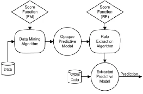
called G-REX (Genetic Rule EXtraction) [5]. G-REX is a black-box rule extraction algorithm; i.e. the overall idea is to treat the opaque model as an oracle and view rule extraction as a learning task, where the target concept is the function learnt by the opaque model. Hence rule sets extracted directly map inputs to outputs. Black-box techniques typically use some symbolic learning algorithm, where the opaque model is used to generate target values for the training examples. The easiest way to understand the process is to regard black-box rule extraction as an instance of predictive modeling, where each input-output pattern consists of the original input vector and the corresponding prediction from the opaque model. From this perspective, black-box rule extraction becomes the task of modeling the function from (original) input attributes to the opaque model predictions; see Figure 1 below.

Data Data Mining Algorithm Opaque Predictive Model Novel Data Prediction Rule Extraction Algorithm Extracted Predictive Model Score Function (PM) Score Function (RE)

Figure 1: Black-box rule extraction

One inherent advantage of black-box approaches, is the ability to extract rules from arbitrary opaque models, including ensembles.

The extraction strategy used by G-REX is based on GP. More specifically, a population of candidate rules is continuously evaluated according to how well the rules mimic the opaque model. The best rules are kept and combined using genetic operators to raise the fitness (performance) over time. After many generations (iterations) the most fit program (rule) is chosen as the extracted rule.

One key property of G-REX is the ability to use a variety of different representation languages, just by choosing suitable function and terminal sets. G-REX has previously been used to extract, for instance, decision trees, regression trees, Boolean rules and fuzzy rules. Another, equally important, feature is the possibility to directly balance accuracy against comprehensibility by using an appropriate fitness function. Although comprehensibility is a rather complex criterion, the simple choice to evaluate comprehensibility using the size of the model is the most

Increasing Rule Extraction Accuracy by Post-processing GP Trees

accepted. Consequently, a typical G-REX fitness function includes a positively weighted fidelity term and a penalty for longer rules. For a summary of the G-REX technique and previous studies, see [6].

GP has in many studies proved to be a very efficient search strategy. Often, GP results are comparable to, or even better than, results obtained by more specialized techniques. One particular example is when GP is used for classification, and the performance is compared to, for instance, decision tree algorithms or rule inducers. Specifically, several studies show that decision trees evolved using GP often are more accurate than trees induced by standard techniques like C4.5/C5.0 [7] and CART [8]; see e.g. [9] and [10]. The main reason for this is that GP is a global optimization technique, while decision tree algorithms typically choose splits greedily, working from the root node down. Informally, this means that GP often will make some locally sub-optimal splits, but the overall model will still be more accurate and more general.

On the other hand, GP search is locally much less informed; i.e. each split is only optimized as a part of the entire decision tree. In addition, GP is not able to find all possible splits, simply because the number of constants available to the GP is limited. This problem is actually accentuated in the later stages of evolution, when populations tend to become more homogenous. With this in mind, the main purpose of this study is to investigate whether some straightforward post-processing techniques, where explicit searching is used to find optimal splits, can improve the performance of GP-induced decision trees.

II. BACKGROUND AND RELATED WORK

Eggermont, Kok and Kosters in two papers evaluate a refined GP-representation for classification, where the search space is reduced by letting the GP only consider a fixed number of possible splits for each attribute; see [11] and [12]. More specifically, a global set of threshold values for each numerical attribute is determined, and then only these threshold values are used in evolution. It should be noted that the threshold values are chosen globally instead of at each specific node. In the two papers, a maximum of five thresholds are selected for every attribute, and both information gain and information gain ration are evaluated as criteria for the selection. Although the results are somewhat inconclusive, the proposed technique are generally more accurate than both C4.5 and standard GP.

As mentioned above, the normal result of rule extraction is another predictive model (the extracted model) which in turn, is used for actual prediction. At the same time, it is important to realize that the opaque model normally is a very accurate model of the relationship between input and target variables. Furthermore; the opaque model could be used to generate predictions for novel instances with unknown target values, as they become available. Naturally, these instances could also be used by the rule extraction algorithm, which is a major difference compared to techniques directly building

transparent models from the dataset, where each training instance must have a known target value. Despite this, all rule extraction algorithms that the authors are aware of, use only training data (possibly with the addition of artificially generated instances) when extracting the transparent model. We have previously argued that a data miner often might benefit from also using test data together with predictions from the opaque model when performing rule extraction. Below, test data inputs together with test data predictions from the opaque model is termed oracle data, with the motivation that the predictions from the opaque model (the oracle) are regarded as ground truth during rule extraction. Naturally, target values for test data are by definition not available when performing rule extraction, but often input values and predictions from the opaque model could be. With access to a sufficiently sized oracle dataset, the rule extraction algorithm could either use only oracle data or augment the training data with oracle instances.

The use of oracle data was first suggested in [13], and further evaluated in [14]. The main result was that rules extracted using oracle data were significantly more accurate than both rules extracted by the same rule extraction algorithm (using training data only) and standard decision tree algorithms; i.e. rules extracted using oracle data explained the predictions made on the novel data better than rules extracted using training data only.

Since the use of oracle data means that the same novel data instances used for actual prediction also are used by the rule extraction algorithm, the problem must be one where predictions are made for sets of instances rather than one instance at a time. This is a description matching most data mining problems, but not all. One example, where a sufficiently sized oracle dataset would not be available, is a medical system where diagnosis is based on a predictive model built from historical data. In that situation, test instances (patients), would probably be handled one at a time. On the other hand, if, as an example, a predictive model is used to determine the recipients of a marketing campaign, the oracle dataset could easily contain thousands of instances. Since the use of oracle data has proven to be beneficial for rule extraction using G-REX, we in this study evaluate the suggested post-processing techniques on trees extracted both with and without the use of oracle data.

III. METHOD

The overall idea introduced in this paper is to post-process GP trees; i.e. only the winning tree is potentially modified. In this study, the GP trees are extracted from opaque models using G-REX. When searching for possible modifications, the structure of the tree is always intact; as a matter of fact, in this study, only the constants in the interior node splits can be modified. More specifically, the post-processing explicitly searches for constant values that would increase the accuracy, one node at a time. The algorithm is presented in pseudo code in Figure 2 below:

do

currentAcc = evaluateTree(tree); foreach interior node

constant=findBestSplit(node, instances); modifyNode(&node, constant);

newAcc = evaluateTree(tree); while (newAcc > currentAcc)

Figure 2: Post-processing algorithm

At the heart of the algorithm is the function findBestSplit, which takes the current node and the instances reaching that node as arguments. The function should return the best constant value to use in the current split. If, as an example, the node is If x1 > 7.5 the function will try alternative values for 7.5, and return the value resulting in the highest accuracy. Which values to consider are determined from the instances reaching the node. In the preceding example, all unique values for x1, found in the instances reaching the node, would be tested. It must be noted that the evaluation always starts with the value found by the GP, so post-processing can never decrease accuracy, only increase it. Clearly, different criteria (like information gain) could be used when evaluating the potential splits, but here we use accuracy; i.e. the split is modified if and only if the modified tree classifies more instances correctly.

Changing splits will, of course, affect which instances that reach each node, so when all nodes have been processed, another sweep could very well further increase accuracy. Consequently, the entire procedure is repeated until there is no change in accuracy between two runs.

When modifying the interior nodes, we could start at the root node or at the leaves. In either case, the question in each node is whether it is possible to increase the overall accuracy by finding a split that changes the distribution of instances to the children; i.e. we assume that all nodes further down the tree will remain as they are. The difference is whether the children are optimized before or after their parent. If we start at the root node, we would first optimize that split, and then proceed down the tree. Or, more generally, when we get to a specific node, the parent node is always already modified, but the children are not. When processing the tree in this manner, we are in fact performing a preorder traversal; see Figure 3 below. The numbers in the squares show the order in which the nodes are processed.

Figure 3: Preorder traversal

If we instead start at the leaves, no node will be optimized before its descendants. Using this strategy, we perform a postorder traversal; see Figure 4 below.

Figure 4: Postorder traversal

A. G-REX settings

The opaque models used to rule extract from are ANN ensembles each consisting of 15 independently trained ANNs. All ANNs are fully connected feed-forward networks where a localist (1-of-C) representation is used. Of the 15 ANNs, seven have one hidden layer and the remaining eight have two hidden layers. The exact number of units in each hidden layer is slightly randomized, but is based on the number of inputs and classes in the current dataset. For an ANN with one hidden layer, the number of hidden units is determined from (1) below.

2 ( )

h

¡

_¢

°

_±

1 (v c) / 2 4rand( (v c) / )c

h ¡¡¢ ¸ ¸ ¸ °°± (2)

2 rand( (v c) / )c c

h ¡¡¢ ¸ ¸ °°± (3) Some diversity is introduced by using ANNs with different architectures, and by training each network on slightly different data. More specifically, each ANN uses a “bootstrap” training set; i.e. instances are picked randomly, with replacement, from the available data, until the number of training instances is equal to the size of the available training set. The result is that approximately 63% of the available training instances are actually used. Averaging is used to determine ensemble classifications.

When using GP for rule extraction, the available functions, F, and terminals T, constitute the literals of the representation language. Functions will typically be logical or relational operators, while the terminals could be, for instance, input variables or constants. Here, the representation language is very similar to basic decision trees; see the grammar presented using Backus-Naur form in Figure 5 below.

F = {if, ==, <, >}

T = {i1, i2, …, in, c1, c2, …, cm, ℜ}

DTree :- (if RExp Dtree Dtree) | Class RExp :- (ROp ConI ConC) | (== CatI CatC) ROp :- < | >

CatI :- Categorical input variable ConI :- Continuous input variable

Class :- Class label

CatC :- Categorical attribute value

ConC :- ℜ

Figure 5: G-REX representation language used

The GP settings used for G-REX in this study are given in Table I below.

TABLE I GP PARAMETERS

Parameter Value Parameter Value

Crossover rate 0.8 Creation depth 7 Mutation rate 0.01 Creation method Ramped half-and-half Population size 1500 Fitness function Fidelity - length penalty Generations 100 Selection Roulette wheel

Persistence 25 Elitism Yes

B. Datasets

The 22 datasets used are all publicly available from the UCI Repository [15]. For a summary of dataset characteristics see Table II below. Instances is the total number of instances in the dataset. Classes is the number of output classes in the dataset. Cont. is the number of continuous input variables and Cat. is the number of categorical input variables.

TABLE II DATASET CHARACTERISTICS

Dataset Instances Classes Cont. Cat.

Breast cancer (Bcancer) 286 2 0 9 Bupa liver disorders (Bupa) 345 2 6 0 Cleveland heart disease (Cleve) 303 2 6 7

Cmc 1473 3 2 7

Crx 690 2 6 9

German 1000 2 7 13

Heart disease Statlog (Heart) 270 2 6 7

Hepatitis (Hepati) 155 2 6 13

Horse colic (Horse) 368 2 7 15

Hypothyroid (Hypo) 3163 2 7 18

Iono 351 2 34 0

Iris 150 3 4 0

Labor 57 2 8 8

Pima Indian diabetes (PID) 768 2 8 0

Sick 2800 2 7 22

Sonar 208 2 60 0

Tae 151 3 1 4

Tictactoe 958 2 0 9

Vehicle 846 4 18 0

Wisconsin breast cancer (WBC) 699 2 9 0

Wine 178 3 13 0

Zoo 100 7 0 16

It is obvious that the post-processing algorithms suggested can affect mainly splits with continuous attributes. When searching for a categorical split, the alternative values actually represent totally different splits; e.g. X1 == 3 instead of X1 == 5. It is, therefore, quite unlikely that there are better categorical splits than the ones found by the GP.

With this in mind, we first considered using only datasets with mainly continuous attributes. Ultimately, though, we decided to include also datasets with mostly categorical attributes, to confirm our reasoning. Having said that, we did not expect the post-processing algorithms to actually modify any trees from the Bcancer, Tictactoe and Zoo datasets.

C. Experiments

As mentioned above, the post-processing techniques are evaluated on G-REX trees extracted both with and without the use of oracle data. Consequently, three experiments are conducted, each comparing three different options for post-processing; No, Pre and Post. No post-processing is exactly that; i.e. the G-REX tree obtained is evaluated on test data without modifications. Pre and Post apply the algorithm described in Figure 2 to the tree obtained from G-REX, before the potentially modified tree is evaluated on test data. Naturally, the processing of the nodes is performed in preorder and postorder, respectively. So, to iterate, on each fold, both post-processing algorithms start from the same G-REX tree. This tree is also evaluated to obtain the result for No. The difference between the three experiments is whether oracle data is used or not. When G-REX original is used, rules are extracted using training data only. G-REX all means that both training data and oracle data are used. G-REX oracle, finally, uses only oracle data. For a summary, see Table III below. For the evaluation, stratified 10-fold cross-validation is used.

TABLE III EXPERIMENTS

Experiment Data used for rule extraction

G-REX original Training G-REX all Training and Oracle

G-REX oracle Oracle

IV. RESULTS

Table IV below shows fidelity results. It should be noted that fidelity values were calculated on the exact data used by G-REX; i.e. for original training data only, for all both training and oracle data, and for oracle, oracle data only.

TABLE IV FIDELITY

Datasets Original All Oracle

No Pre Post No Pre Post No Pre Post

Bcancer .847 .847 .847 .855 .855 .855 .986 .986 .986 Bld .774 .799 .797 .769 .781 .782 .918 .924 .924 Cleve .861 .863 .863 .859 .862 .862 .977 .977 .977 Cmc .783 .789 .790 .792 .803 .803 .817 .826 .826 Crx .919 .921 .922 .923 .924 .924 .958 .958 .958 German .784 .787 .787 .789 .792 .792 .882 .886 .886 Heart .868 .871 .871 .869 .870 .870 .989 .989 .989 Hepati .883 .886 .886 .890 .898 .897 1.00 1.00 1.00 Horse .871 .873 .873 .879 .879 .879 .972 .972 .972 Hypo .986 .988 .988 .988 .990 .990 .993 .993 .993 Iono .932 .940 .940 .937 .946 .946 .986 .986 .986 Iris .979 .983 .983 .977 .981 .981 1.00 1.00 1.00 Labor .988 .988 .988 .982 .984 .984 1.00 1.00 1.00 PID .887 .896 .896 .885 .894 .894 .941 .946 .946 Sick .983 .985 .985 .983 .984 .984 .987 .988 .988 Sonar .827 .843 .843 .812 .828 .826 1.00 1.00 1.00 Tae .704 .719 .720 .693 .702 .701 .953 .953 .953 Tictactoe .810 .810 .810 .804 .804 .804 .877 .877 .877 Vehicle .637 .654 .654 .628 .651 .652 .743 .760 .760 Wbc .973 .974 .974 .976 .977 .977 .996 .996 .996 Wine .961 .967 .968 .960 .974 .974 1.00 1.00 1.00 Zoo .923 .923 .923 .916 .916 .916 .990 .990 .990 From Table IV, it is obvious that the post-processing algorithm was able to find better splits and thereby increasing fidelity. As a matter of fact, when using only training data, the post-processing algorithm increased the fidelity on all datasets but the three “categorical only” mentioned above. This does not mean that the post-processing algorithm always was able to modify the trees, on several datasets there were, in fact, no modifications on a large majority of the folds.

When using oracle data only, the number of instances in the fitness set is quite small, so the fidelity of the starting tree is normally quite high. For five datasets (Hepati, Iris, Labor, Sonar and Wine) the fidelity is even a perfect 1.0 to start with. Because of this, it is not surprising that there are relatively few improvements found.

When using all data, the starting tree has most often, but not always, a higher fidelity, compared to the tree extracted using training data only. Still, the post-processing managed to increase fidelity on all datasets but the three “categorical-only” and Horse. Often, however, the increase is quite small, sometimes even the result of a single modification, on just one fold. Overall, however, the picture is clearly that the suggested algorithm was capable of increasing fidelity.

Naturally, fidelity is not vital per se, the important question is whether the modifications would also increase test set accuracies. Table V below shows test set accuracies. The results obtained by the neural network ensemble used to rule extract from are included for comparison.

TABLE V TEST ACCURACIES

Datasets Ensemble Original All Oracle

No Pre Post No Pre Post No Pre Post

Bcancer .729 .725 .725 .725 .714 .714 .714 .736 .736 .736 Bld .721 .635 .665 .659 .641 .624 .626 .691 .697 .697 Cleve .807 .770 .777 .777 .807 .810 .810 .810 .810 .810 Cmc .551 .547 .565 .565 .551 .549 .551 .539 .540 .540 Crx .859 .849 .854 .854 .848 .851 .851 .849 .849 .849 German .749 .716 .720 .722 .726 .728 .728 .737 .735 .735 Heart .793 .785 .789 .789 .785 .785 .785 .804 .804 .804 Hepati .860 .807 .807 .807 .833 .840 .840 .860 .860 .860 Horse .817 .842 .844 .844 .847 .847 .847 .806 .806 .806 Hypo .983 .979 .981 .981 .980 .982 .982 .980 .980 .980 Iono .934 .877 .889 .889 .914 .929 .926 .926 .926 .926 Iris .967 .953 .953 .953 .947 .960 .960 .967 .967 .967 Labor .940 .840 .840 .840 .920 .920 .920 .940 .940 .940 PID .767 .746 .753 .754 .753 .755 .757 .750 .747 .747 Sick .970 .971 .973 .973 .971 .970 .970 .967 .968 .968 Sonar .865 .700 .740 .740 .730 .750 .745 .865 .865 .865 Tae .567 .460 .480 .480 .480 .473 .473 .547 .547 .547 Tictactoe .898 .736 .736 .736 .752 .752 .752 .781 .781 .781 Vehicle .848 .582 .586 .587 .605 .618 .623 .664 .676 .676 Wbc .964 .957 .958 .958 .959 .959 .959 .965 .965 .965 Wine .965 .918 .918 .929 .929 .953 .953 .965 .965 .965 Zoo .950 .880 .880 .880 .920 .920 .920 .940 .940 .940 Table V shows that on a majority of datasets, the increase in fidelity also led to an increase in test set accuracy. Again, it must be noted that these result do not mean that test set accuracies were always increased. As a matter of fact, on several folds, an increase in fidelity led to no change in accuracy. On some folds, the increase in fidelity even led to lower accuracy. When aggregating the results over all ten folds, however, the results are very promising for the suggested algorithm. To further analyze the result, the two post-processing algorithms were pair-wise compared to each other and No, one experiment at a time. Table VI - VIII below show these comparisons for the three experiments. The values tabulated are datasets won, lost and tied, for the row technique when compared to the column technique. Using 22 data sets, a standard sign-test (α=0.05) requires 16 wins for statistical significance. When using a sign test, ties are split evenly between the two techniques. Statistically significant differences are shown using bold and underlined values.

TABLE VI

WINS, LOSSES AND TIES USING G-REX ORIGINAL

No Pre Post

W L T W L T W L T

No - - - 0 15 7 0 16 6

Pre 15 0 7 - - - 1 4 17

Post 16 0 6 4 1 17 - - -

First of all, it is interesting to note that neither post-processing algorithm lose a single dataset against No. The sign test consequently shows that both algorithms are significantly more accurate than using no post-processing. The results also show that, on a large majority of the datasets, there is no difference between Pre and Post.

TABLE VII

WINS, LOSSES AND TIES USING G-REX ALL

No Pre Post

W L T W L T W L T

No - - - 4 11 7 3 11 8

Pre 11 4 7 - - - 3 4 15

Post 11 3 8 4 3 15 - - -

Here, a sign test, reports no statistically significant differences. Still, it is clearly beneficial to use the post-processing algorithm, even for G-REX all. As a matter of fact, if the three “categorical only” data sets were removed before the analysis, the use of either Pre or Post, would again be significantly more accurate than No.

TABLE VIII

WINS, LOSSES AND TIES USING G-REX ORACLE

No Pre Post

W L T W L T W L T

No - - - 3 5 14 3 5 14

Pre 5 3 14 - - - 0 0 22

Post 5 3 14 0 0 22 - - -

For G-REX oracle, the picture is quite different. Here, there is generally very little to gain by using the post-processing suggested. The reason is, of course, the very high fidelity obtained by the rule extraction to start with. Still, it could be noted that the post-processing was able to increase accuracy on five data sets. For two of these (Bld and Vehicle) the increase is not negligible; see Table V.

V. CONCLUSIONS

We have in this paper suggested a novel algorithm for post-processing of GP trees. The technique iteratively, one node at a time, searches for possible modifications that would result in higher accuracy. More specifically, for each split, the algorithm evaluates every possible constant value and chooses the best. It should be noted that the algorithm can only increase accuracy (on training data), since modifications are only carried out when the result is a more accurate tree.

In this study, we evaluated the algorithm using the rule extraction technique G-REX. Results show that when the rule extraction uses only training data, the post-processing increased accuracy significantly. When using both training and oracle data, it is still clearly advantageous to apply the post-processing. Even when starting from a tree extracted using oracle data only, the post-processing is sometimes capable of increasing accuracy. Overall, the very promising picture is that the post-processing more often than not increases accuracy, and only very rarely decreases it.

VI. DISCUSSION AND FUTURE WORK

In this study, we applied the novel technique to rule extraction, but it could, of course, just as well, be used on any GP classification tree. So, one obvious future study is to evaluate the suggested technique on GP classification. Another study is to investigate whether it would be beneficial to search for an entire new split, not just a

constant value. In that study, it would be natural to also evaluate different criteria (like information gain) as alternatives to accuracy. This would, however, be very similar to standard decision tree algorithms. The challenge is to find the right mix between the locally effective greed in decision tree algorithms and the global optimization in GP.

Finally, we have also performed some initial experiments, with promising results, where the algorithm suggested was instead used as a mutation operator during evolution. Potential benefits are higher accuracy or faster convergence.

ACKNOWLEDGMENT

This work was supported by the Information Fusion Research Program (University of Skövde, Sweden) in partnership with the Swedish Knowledge Foundation under grant 2003/0104 (URL: http://www.infofusion.se).

REFERENCES

[1] H. Lu, R. Setino and H. Liu, Neurorule: A connectionist approach to data mining, International Very Large Databases Conference, pp. 478-489, 1995.

[2] M. Craven and J. Shavlik, Extracting Tree-Structured Representations of Trained Networks, Advances in Neural Information Processing

Systems, 8:24-30, 1996.

[3] R. Andrews, J. Diederich and A. B. Tickle, A survey and critique of techniques for extracting rules from trained artificial neural networks,

Knowledge-Based Systems, 8(6), 1995.

[4] M. Craven and J. Shavlik, Rule Extraction: Where Do We Go from Here?, University of Wisconsin Machine Learning Research Group

working Paper, 99-1, 1999.

[5] U. Johansson, R. König and L. Niklasson, Rule Extraction from Trained Neural Networks using Genetic Programming, 13th

International Conference on Artificial Neural Networks, Istanbul,

Turkey, supplementary proceedings pp. 13-16, 2003.

[6] U. Johansson, Obtaining accurate and comprehensible data mining

models: An evolutionary approach, PhD thesis, Institute of

Technology, Linköping University, 2007.

[7] J. R. Quinlan, C4.5: Programs for Machine Learning, Morgan Kaufmann, 1993.

[8] L. Breiman, J. H. Friedman, R. A. Olshen and C. J. Stone,

Classification and Regression Trees, Wadsworth International, 1984.

[9] A. Tsakonas, A comparison of classification accuracy of four genetic programming-evolved intelligent structures, Information Sciences, 176(6):691-724, 2006.

[10] C. C. Bojarczuk, H. S. Lopes and A. A. Freitas, Data Mining with Constrained-syntax Genetic Programming: Applications in Medical Data Sets, Intelligent Data Analysis in Medicine and Pharmacology -

a workshop at MedInfo-2001, 2001.

[11] J. Eggermont, J. Kok and W. A. Kosters, Genetic Programming for Data Classification: Refining the Search Space, 15th

Belgium/Neth- erlands Conference on Artificial Intelligence, pp. 123-130, 2003.

[12] J. Eggermont, J. Kok and W. A. Kosters, Genetic Programming for Data Classification: Partitioning the Search Space, 19th

Annual ACM Symposium on Applied Computing (SAC'04), pp. 1001-1005, 2004. [13] U. Johansson, T. Löfström, R. König and L. Niklasson, Why Not Use

an Oracle When You Got One?, Neural Information Processing -

Letters and Reviews, Vol. 10, No. 8-9: 227-236, 2006.

[14] U. Johansson, T. Löfström, R. König, C. Sönströd and L. Niklasson, Rule Extraction from Opaque Models – A Slightly Different Perspective, 6th

International Conference on Machine Learning and Applications, Orlando, FL, IEEE press, pp. 22-27, 2006.

[15] C. L. Blake and C. J. Merz, UCI Repository of machine learning

databases, University of California, Department of Information and