Method Evaluation of Global-Local Finite
Element Analysis
Gabriella Ahlbert
Master thesis in Solid Mechanics performed at Linköping University
Method Evaluation of Global-Local Finite Element Analysis
Gabriella AhlbertStudent reviewer: Emil Sandgren Supervisor Saab: Lars Djärv
Supervisor Linköping University: Kjell Simonsson Examiner Linköping University: Sören Sjöström
COPYRIGHT
The publishers will keep this document online on the Internet – or its possible replacement – for a period of 25 years starting from the date of publication barring exceptional circumstances. The online availability of the document implies permanent permission for anyone to read, to download, or to print out single copies for his/hers own use and to use it unchanged for non-commercial research and educational purpose. Subsequent transfers of copyright cannot revoke this permission. All other uses of the document are conditional upon the consent of the copyright owner. The publisher has taken technical and administrative measures to assure authenticity, security and accessibility.
According to intellectual property law the author has the right to be mentioned when his/her work is accessed as described above and to be protected against infringement.
For additional information about the Linköping University Electronic Press and its procedures for publication and for assurance of document integrity, please refer to its www home page:
http://www.ep.liu.se/.
Avdelning, Institution
Division, Department Division of Solid Mechanics
Department of Management and Engineering Linköpings universitet
SE-583 83 Linköping, Sweden
Datum Date 2012-06-21 Språk Language Svenska/Swedish X Engelska/English Antal sidor Number of Pages 78 Rapporttyp Report Category Licentiatavhandling X Examensarbete C-uppsats D-uppsats Rapport
Serietitel och serienummer
Title of Series, Numbering
ISRN: LIU-IEI-TEK-A--12/01287—SE
URL, Elektronisk Version
URL, Electronic Version
http://urn.kb.se/resolve?urn=urn:nbn:se:liu:diva-78103
Titel
Title
Författare
Author
Method Evaluation of Global-Local Finite Element Analysis Gabriella Ahlbert
Sammanfattning
Abstract
When doing finite element analysis upon the structure of Saab’s aircrafts a coarse global model of mainly shell elements is used to determine the load distribution for sizing the structure. At some parts of the aircraft it is, however, desirable to implement a more detailed analysis. These areas are usually modelled with solid elements; the problem of connecting the fine local solid elements to the coarse global model with shell elements then arises. This master thesis is preformed to investigate possible Global-Local methods to use for the structural analysis on Gripen, on of the latest generations of Saabs aircrafts. First a literature study of current methods on the market is made, thereafter a few methods are implemented on a generic test structure and later on also tested on a real detail of Gripen VU. The methods tested in this thesis are Mesh refinement in HyperWorks, RBE3 in HyperWorks, Glue in MSC Patran/Nastran and DMIG in MSC Nastran. The software is however not evaluated in this thesis, and a further investigation is recommended to find the most fitting software for this purpose. All analysis are performed with linear assumptions.
Mesh refinement is an integrated technique where the elements are gradually decreasing in size. Per definition, this technique cannot handle gaps, but it has almost identical results to the fine reference model.
RBE3 is a type of rigid body element with zero stiffness, and is used as an interface element. RBE3 is possible to use for both Shell-To-Shell and Shell-To-Solid couplings, and can handle offsets and gaps in the boundary between the global and local model.
Glue is a contact definition and is also available in other software under other names. The global and the local model is defined as contact bodies and a contact table is used to control the coupling. Glue works for both Shell-To-Shell and Shell-To-Shell-To-Solid couplings, but has problems dealing with offsets and gaps in the boundary between the global and local model.
DMIG is a superelement technique where the global model is divided into smaller sub-models which are mathematically connected. DMIG is only possible to use when the nodes on the boundary of the local model have the same position as the nodes at the boundary of the global model. Thus, it is not possible to only use DMIG as a Global-Local method, but can advantageously be combined with other methods.
The results indicate that the preferable method to use for Global-Local analysis is RBE3. To decrease the size of the files and demand for computational power, RBE3 can be combined with a superelement technique, for example DMIG.
Finally, it is important to consider the size of the local model. There will inevitably be boundary effect when performing a Global-Local analysis of the suggested type, and it is therefore important to make the local model big
ABSTRACT
When doing finite element analysis upon the structure of Saab’s aircrafts a coarse global model of mainly shell elements is used to determine the load distribution for sizing the structure. At some parts of the aircraft it is, however, desirable to implement a more detailed analysis. These areas are usually modelled with solid elements; the problem of connecting the fine local solid elements to the coarse global model with shell elements then arises.
This master thesis is preformed to investigate possible Global-Local methods to use for the structural analysis on Gripen, on of the latest generations of Saabs aircrafts. First a literature study of current methods on the market is made, thereafter a few methods are implemented on a generic test structure and later on also tested on a real detail of Gripen VU. The methods tested in this thesis are Mesh refinement in HyperWorks, RBE3 in HyperWorks, Glue in MSC Patran/Nastran and DMIG in MSC Nastran. The software is however not evaluated in this thesis, and a further investigation is recommended to find the most fitting software for this purpose. All analysis are performed with linear assumptions.
Mesh refinement is an integrated technique where the elements are gradually decreasing in size. Per definition, this technique cannot handle gaps, but it has almost identical results to the fine reference model.
RBE3 is a type of rigid body element with zero stiffness, and is used as an interface element. RBE3 is possible to use for both Shell-To-Shell and Shell-To-Solid couplings, and can handle offsets and gaps in the boundary between the global and local model.
Glue is a contact definition and is also available in other software under other names. The global and the local model is defined as contact bodies and a contact table is used to control the coupling. Glue works for both Shell-To-Shell and Shell-To-Solid couplings, but has problems dealing with offsets and gaps in the boundary between the global and local model.
DMIG is a superelement technique where the global model is divided into smaller sub-models which are mathematically connected. DMIG is only possible to use when the nodes on the boundary of the local model have the same position as the nodes at the boundary of the global model. Thus, it is not possible to only use DMIG as a Global-Local method, but can advantageously be combined with other methods.
The results indicate that the preferable method to use for Global-Local analysis is RBE3. To decrease the size of the files and demand for computational power, RBE3 can be combined with a superelement technique, for example DMIG.
Finally, it is important to consider the size of the local model. There will inevitably be boundary effect when performing a Global-Local analysis of the suggested type, and it is therefore important to make the local model big enough so that the boundary effects have faded before reaching the area of interest.
PREFACE
In this master thesis different methods of Global-Local finite element techniques are evaluated. The work has been carried out at Saab Aeronautics, Linköping during spring 2012.
By this thesis, I will conclude my studies in mechanical engineering at Linköping University, Sweden, with a degree in Master of Science in Mechanical Engineering.
I would like to thank everyone who have helped and supported me during this project. Special thanks to my supervisors Lars Djärv at Saab Aeronautics and Professor Kjell Simonsson at
Linköping University for the commitment and support during the entire project. I would also like to thank Marcus Henriksson at Saab Aeronautics, my examiner Professor Sören Sjöström and my student reviewer Emil Sandgren for helpful comments on the thesis.
Lastly, I would also like to thank all those who have helped and supported me during my academic years at Linköping University; classmates, friends, family and teachers. All of you have supported and helped me to perform my best.
Gabriella Ahlbert Linköping June 2012
CONTENTS
CHAPTER 1 INTRODUCTION... 1
1.1 SAAB... 1
1.2 OBJECTIVE... 1
1.2.1 The Global Model of Gripen... 2
1.2.2 The Local Models of Gripen ... 2
1.3 PROCEDURE... 2
1.4 SOFTWARE... 3
1.5 RESTRICTIONS... 4
CHAPTER 2 THEORY... 5
2.1 FUNDAMENTALS OF FINITE ELEMENT ANALYSIS... 5
2.2 MULTISCALE ANALYSIS... 7 2.2.1 Displacement Approach... 8 2.2.2 Force Approach ... 8 2.3 INTEGRATED ANALYSIS... 8 2.3.1 Mesh Refinement ... 8 2.3.2 Interface Elements... 9 2.3.3 Rigid Elements ... 9 2.3.4 Multipoint Constraints... 10 2.3.5 Glue Constraint... 10
2.3.6 Shell-To-Solid Coupling in Abaqus ... 11
2.4 SUPERELEMENTS... 11
2.4.1 Static Condensation... 12
2.4.2 Direct Matrix Input ... 12
CHAPTER 3 GENERIC MODEL AND EVALUATION CRITERIA... 13
3.1 THE GLOBAL MODEL... 13
3.1.1 Material ... 15
3.2 THE LOCAL MODELS... 15
3.2.1 Case 1: Shell Elements ... 16
3.2.2 Case 2: Solid Elements ... 16
3.2.3 Case 3: Offset With Shell Elements ... 17
3.2.4 Case 4: Offset With Solid Elements... 19
3.3 REFERENCE MODEL... 20
3.4 LOAD CASES AND BOUNDARY CONDITIONS... 20
3.5 EVALUATION OF THE RESULTS... 22
3.5.1 Evaluation Criterion 1 - Connection ... 22
3.5.2 Evaluation Criterion 2 – Displacements... 23
3.5.3 Evaluation Criterion 3 – Stresses... 23
3.5.4 Calculations of Individually Criterion Scores... 24
3.5.5 Total Criterion Score... 25
4.1.1 Displacement Diagrams ... 29
4.1.2 Stress Diagram... 30
4.2 MESH REFINEMENT... 31
4.3 RBE3 ... 33
4.3.1 Case 1: Shell Elements ... 35
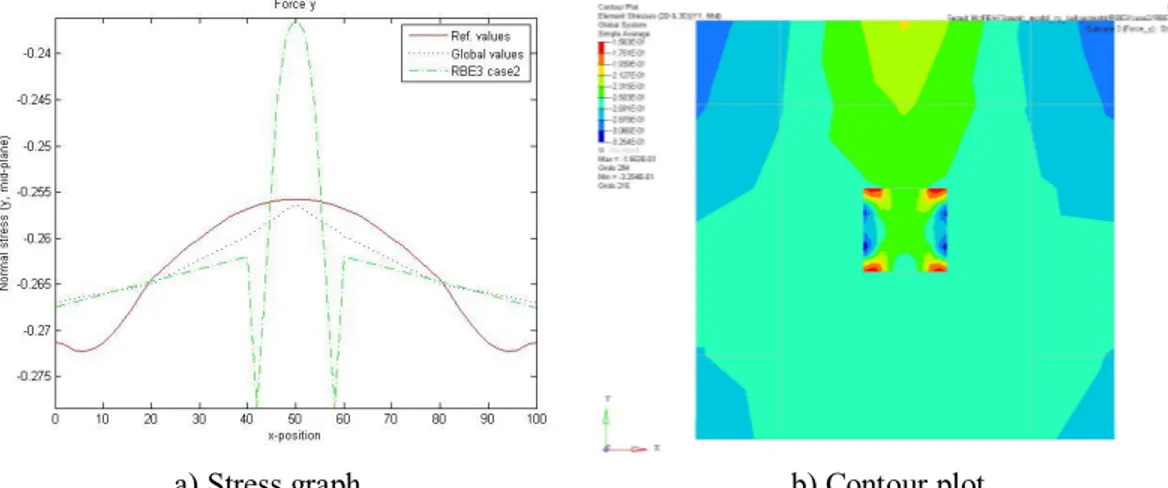
4.3.2 Case 2: Solid Elements ... 39
4.3.3 Case 3: Offset With Shell Elements ... 42
4.3.4 Case 4: Offset With Solid Elements... 42
4.4 GLUE... 45
4.4.1 Case 1: Shell Elements ... 45
4.4.2 Case 2: Solid Elements ... 47
4.4.3 Case 3: Offset With Shell Elements ... 48
4.4.4 Case 4: Offset With Solid Elements... 48
4.5 DMIG... 51
4.5.1 DMIG with Mesh Refinement... 51
4.5.2 DMIG with RBE3 ... 53
CHAPTER 5 GRIPEN TEST STUDY ... 57
5.1 MODEL DESCRIPTION... 57
5.2 LOAD CASES AND BOUNDARY CONDITIONS... 58
5.3 GLOBAL MODEL... 59
5.4 REFERENCE MODEL... 60
5.5 MESH REFINEMENT... 61
5.6 RBE3 ... 62
5.7 RESULTS... 64
CHAPTER 6 EVALUATION AND CONCLUSIONS... 67
6.1 EVALUATION OF PARAMETRIC STUDY... 67
6.1.1 Mesh Refinement ... 67
6.1.2 RBE3... 67
6.1.3 Glue... 68
6.1.4 DMIG ... 68
6.1.5 Comparison of methods ... 69
6.2 EVALUATION OF GRIPEN TEST STUDY... 72
CHAPTER 7 DISCUSSION ... 73
7.1 RECOMMENDATION OF METHOD... 74
CHAPTER 8 FUTURE WORK ... 75
APPENDIX A MATLAB SCRIPT FOR EVALUATION OF THE PARAMETRIC STUDY ...A.1
A.1 DISP_RESULTS_MAIN.M...A.1
A.2 PLOT_DISP.M...A.5
A.3 CRIT_DISP.M...A.7
APPENDIX B RESULTS FROM PARAMETRIC STUDY...B.1
B.1 CONNECTION SCORES...B.2
B.2 DISPLACEMENT SCORES...B.3
B.3 STRESS SCORES...B.6
B.4 TOTAL SCORES...B.9
APPENDIX C RESULTS FROM GRIPEN TEST STUDY ...C.1
C.1 GLOBAL RESULTS...C.1
C.2 RESULTS FROM MESH REFINEMENT...C.3
C.3 RESULTS FROM RBE3...C.5
APPENDIX D USER GUIDE TO USED METHODS...D.1
D.1 MESH REFINEMENT...D.1
D.2 RBE3 ...D.1
D.2.1 Automated Script...D.2 D.2.2 Manual Method...D.4
D.3 GLUE...D.5
D.4 DMIG WITH MESH REFINEMENT...D.9
CHAPTER 1
INTRODUCTION
This chapter is an introduction to the thesis, describing the background, purpose and method for the project.
1.1 Saab
Saab, Svenska Aeroplan Aktiebolaget, was founded in 1937 after a decision of the Swedish government to enlarge the domestic military aircraft industry in Sweden. Since Saab delivered its first aircraft, the light bomber and reconnaissance aircraft B 17, they have had a close cooperation with the Swedish Air Force and have developed several generations of military aircrafts, such as Tunnan, Lansen, Draken, Viggen and Gripen
Jas 39 Gripen, hereafter Gripen, is a multi-role fighter used for fighter, attack and reconnaissance missions. There are four different versions of Gripen of which two are two-seaters. A completely new version of Gripen, under the working name Gripen VU, is now being developed.
Saab is today one of the worlds leading companies in the defence industry with around 12 500 employees and is divided into five business areas, active mostly in Europe, South Africa, Australia and the United states. For further details, see Saabgroup, 2010.
1.2 Objective
A common technique to evaluate the strength of a complex body, such as an aircraft, is to perform a finite element analysis. It is not a technique that can completely replace the physical testing, nevertheless, it is used as much as possible, within what the regulations allow, because of the economical advantages. The finite element method is a numerical simulation techniques and is used in a wide variety of disciplines such as examination of cracks, thermal heating and flutter. The analyses of an aircraft are based on the worst case scenario, for example doing a tough manoeuvre in bad weather.
When doing finite element analysis upon Saab’s aircrafts a global model is used to determine the load distribution for sizing the structure. The global model has a coarse mesh, precluding details in the structure to reduce the computational power and shorten the calculation time. At some parts of the aircraft it is however desirable to implement a more detailed analysis, for instance at
methods in different software to deal with Global-Local analysis, and the aim with this master thesis is to investigate how these methods work and which methods could be suitable for Saab’s Global-Local analyses on Gripen. This thesis is not intended to evaluate different software, although a few specific programs have been used in this study. Many of the methods are also available in other software and it is recommended to do a further investigation if the most fitting software for each method is needed.
1.2.1 The Global Model of Gripen
The global finite element model of Jas 39 Gripen consists mainly of shell elements with beam elements as stiffeners. The shell elements are two-dimensional elements with a surface, thickness and material data such as stiffness and mass, whereas the beam elements are one-dimensional elements that are subjected to traverse and normal load as well as moments. The nodes in the shell elements have six degrees of freedom, translation and rotation in each direction. Other element types that are used in the global model are solid elements for thick sandwich cores, point elements, for mass loads, and spring elements.
The global model has to give a true interpretation of stiffness and mass. Furthermore, it is also used in other disciplines such as calculations of linear dynamic loads, flutter and aero servo elasticity analysis.
1.2.2 The Local Models of Gripen
The local models consist mainly of either shell or solid elements, where solid elements only have three, translational, degrees of freedom.
A local model is for example needed at details including radius with high stress concentrations or details where the geometry is complex. The local model can also be used to implement non-linear calculations, for example when non-linear material properties are needed, or when the geometry is offset.
1.3 Procedure
The thesis start with a thorough literature study of the methods on the market, examples of questions that require answers are following:
Which methods exist today?
Which methods can be implemented in the software used by Saab? How are other companies in the aerospace industry solving this problem?
Figure 1.1: Flowchart over the procedure
Literature study
Parametric
The literature study is followed by a parametric study where some of the methods found in the first step are tested on a generic model. The parametric study will lead to a few preferred methods that are to be applied on a test model from Gripen VU to evaluate the feasibility and effectiveness. A flowchart over the procedure is seen in Figure 1.1.
1.4 Software
Finite element software are built in three parts; a pre-processor in which for example the geometry and mesh can be defined, a solver that is performing the calculations, and a post-processor where the results from the solver ca be displayed in a variety of ways, such as plots and graphs. The process is described in Figure 1.2.
Figure 1.2: Structure of Finite Element software
The pre-processor generates a file with bulk-data, containing all information about the model, mesh, loads etc. This bulk-data file is then sent to a solver. The solver generates for instance a MASTER and DBALL file during the solving process; however these files are usually deleted after solving and replaced by an input file to the post-processor.
The software to be used for this master thesis is not fixed. However, as a pre-processor, HyperMesh or MSC Patran is preferred at Saab and MSC Nastran is preferred as a solver of linear calculations and some nonlinear calculations. Abaqus is usually used for the nonlinear calculations. Post-processing is usually done in the in-house tools DIM and Intplot.
MSC Patran and MSC Nastran are used for the structure analysis of Gripen today, and one of the secondary objectives of this master thesis is to investigate whether the HyperWorks package can be used instead. Due to this, MSC Patran, MSC Nastran and the HyperWorks package will be used in this master thesis. The different software combinations are not mixed; when MSC Patran is used as
Pre-processor
e.g. Patran, HyperMesh
MASTER DBALL Bulk-data xdb op2 Solver
e.g. Nastran, Radioss
Post-processor
For evaluation and comparison of the results in the parametric study, MATLAB is used.
1.5 Restrictions
The thesis shall result in a proposal of one or more suitable methods for Global-Local finite element analysis. Since the displacement and force approaches (multiscale analysis) already have been tested for Gripen, this thesis will have a main focus on integrated analysis and superelements. The multiscale analysis is however still a part of the literature study. The chosen method have to be effective in that way that it must solve the problem as correctly as possible but still be feasible in terms of software, time and money.
The global model of Gripen is modelled in MSC Patran, which means that if an integrated model is to be used, the pre-processor is restricted to MSC Patran unless the global model is exported to another software. A break out model or the superelement approach could however be implemented in an optional program if this procedure is believed to bee advantageous.
CHAPTER 2
THEORY
This chapter describes the basic technique behind Finite Element Analysis in general and Global-Local methods in particular. For more information about each Global-Global-Local technique used in this master thesis, the reader is referred to Appendix D User Guide to Used Methods.
2.1 Fundamentals of Finite Element Analysis
The Finite Element Method (FEM) is today a widely spread computational technique among engineers used to calculate approximate solutions in a large variety of engineering disciplines. According to Torstenfelt, 2008, the history of the method can be traced back to Richard Courant in 1942. As the computer became more common and increasingly better, the method became a more sophisticated method and the word “finite element” was coined by Ray W. Clough in 1960. One of the main driving forces for the development was engineers working in the aeronautical industry and in the 1970s the first commercial finite element package was developed.
Finite element method can be used to solve both partial differential equations and integral equations by either eliminate the differential equation completely or replace it with an ordinary differential equation, which can be solved. The domain is usually a physical structure divided into finite elements with a resulting model called mesh. The variables of interest are computed at the corner points of the elements, which are called nodes. Each node has a given set of degrees of freedom, which is all possible ways the node can move; for example translation or rotation in different coordinate directions.
In finite element analysis, different types of elements are used, where the elements have various dimensions and shapes depending on what properties that are desired, for further information, the reader is referred to Felippa, 2004. Figure 2.1 shows some of the most commonly used element types.
Zero-dimensional elements are point entities that represent for example a point mass. One-dimensional elements have a length but no area, it is placed between two nodes and can
sometimes also have middle nodes as well. Unlike the zero-dimensional element this element can contain material properties, such as density, Young’s modulus, Poisons ratio and geometry features like cross section area and second moments of inertia. The one-dimensional element can be for example a beam or bar.
are quadrilateral and triangular elements. The two-dimensional element can be for example a plate or a shell.
Three-dimensional elements have unlike the two-dimensional elements also a volume. It can
contain material properties and the nodes have three, translational, degrees of freedom. The most common shapes are tetrahedral and hexahedral element.
Figure 2.1: Visualization of the different element types and dimensions
A general rule to obtain a more accurate solution is to increase the number of elements used. The increase of elements is however also affecting the computational needs; according to Kxcad, 2009, the time taken for a matrix solution is proportional to the square of the total number of degrees of freedom of the structure.To overcome this problem, the structure can be divided into sections where Global-Local modelling may be used.
As described in the introduction, when doing finite element analysis upon Gripen, a global model with a coarse mesh is used. The global model is then divided into other local models with a more dense mesh. There are today several different methods to connect the local models to the global models. Figure 2.2 shows a breakdown chart over the classification of methods treated in this report.
The local model can be analyzed as a breakout model physically separated from the global model (multiscale analysis, also called break out modelling) or physically attached to the global model (integrated analysis). A mixture of this two are the Direct Matrix Input approach, where the local model is physically separated from the model but mathematically attached. All methods are explained more thorough below in this section.
The advantages of using superelement, also called sub-structure technique, are mainly three; to be 1D
2D
3D 0D
Figure 2.2: Breakdown chart over Global-Local finite element methods
2.2 Multiscale Analysis
The structures modelled in the aircraft industry are usually of a quite complicated art and the multiscale analysis is therefore a commonly used method in the industry. The essential view of the multiscale analysis is to divide the structure in sub-models which can be edited and simulated parallel to each other. The aircraft is first modelled as a global model with a coarse mesh excluding local details, and is then divided into smaller local models where the mesh usually is finer to give more detailed results.
The multiscale analysis originates from Saint Venant’s principle published in 1855, and later on interpreted by for example von Mises in 1945. The core of the Saint Venant’s principle is that the difference between stresses caused by statically equivalent loads becomes very small at sufficiently large distance from the load. That is, if the boundary is placed at a sufficiently large distance from the area of interest in the local model, the results will not be affected by the absence of the global model. Tests have shown that the boundary effects are insignificant at a distance greater than the largest dimension of the area over which the loads are acting. This is described by Molker, 2012. There are two main ways to execute the multiscale analysis; the displacement approach and the force approach. Commonly to both methods is that boundary conditions between the global and local models are extracted from the global model and used as boundary conditions in the local model. A mixture of the two methods can also be used; a combination of displacements and forces from the global analysis is then extracted as boundary conditions from the global model. This approach is possible to use if the local sub-model is transferring forces in a well defined load path, se Raghavan, Prasanna Kumar, 2008, for further details.
To make sure that the multiscale analysis is accurate a coupled approach can be used. That is, after performing the analysis, the boundary conditions from the local model are transferred to the global model where a new analysis is performed to check if the global model is affected.
There are several ways of extracting the values at the boundary from the global model, one is to use fields in for example MSC Nastran and another one is to use free body diagram which is available in several software such as MSC Patran and HyperWorks. Free body diagram is a tool in the
pre-Global-Local FE-Analysis
Multiscale analysis Integrated analysis Superelements
Displacement approach
Force approach
2.2.1 Displacement Approach
The most common of the multiscale analyses is the displacement approach when displacements are extracted from the global model and used as boundary conditions in the local model, described by Raghavan, 2009. This method is very effective but it has two important limitations. Firstly, the geometry and material properties of the global- and local models have to be the same.
2.2.2 Force Approach
The second approach to perform a multiscale analysis is to use forces and moments as boundary conditions. With this approach, the shortcomings for the displacement method are overcome. The force method gives the local model as a free body diagram, where the forces acting on the sub-model are in self equilibrium.
2.3 Integrated Analysis
To be able to perform optimization on a local detail it is required to simulate the local model within the global model, in these cases an integrated analysis is used. The integrated analysis could be divided into three subgroups, depending on the element types in the global and local model. In Gripen, the global model is built of mainly shell elements, whereas the local models usually consist of mainly solid elements. This is obviously an issue since the different models have nodes with inconsistent degrees of freedom. If the differences in degrees of freedom are not taken into account, the transition will act as a hinge for plate elements or as a pinned connection for bar elements.
When integrated analysis is used, there could be incompatibilities between elements which can result in local stress deviations. Due to this it is important never to place the boundary between the global and local model in or near an area of interest or where the stress variations are large. The area of interest will, however, not be affected if the interface elements are placed far enough apart, according to Saint Venant’s principle, see Von Mises, 1945, for further details.
2.3.1 Mesh Refinement
Mesh refinement is a method that can be used when the global and local model is of the same dimensions, Shell-To-Shell or Solid-To-Solid. When using mesh refinement the density of the coarse global mesh is enhanced. There are three kinds of refinement methods described by Flaherty.
h-refinement: local refinement of a mesh r-refinement: relocating or moving a mesh
p-refinement: varying the polynomial degree of the basis
An example of a mesh refinement is the use of triangular elements as in Figure 2.3. A theoretical alternative to the triangular elements is to delete mid-side nodes; this is however usually a non-advantageous method since it distorts the stress distribution in the elements. If triangular elements are used, it is important to never use the results of these elements because they have increased stiffness. A few triangular elements spread out in the model could however be okay as long as they are not placed in the area of interest.
Figure 2.3: Example of triangular refinement elements
2.3.2 Interface Elements
One alternative to mesh refinement is to us interface elements. The interface method is however also working when the elements in the global and local models are of different dimensions. The interface element makes the displacement of the nodes in the local model slaved to nodes in the global model with multipoint constraints, described below. An example of the principal of interface elements is showed in Figure 2.4 where the middle node in the local model is slaved to the two nodes in the global model. The displacement is interpolated between the two global nods to receive the displacement in the local node. More information about interface elements can be found in MSC Software Corporation, 2012a.
Figure 2.4: Principal of interface element. The displacement of the middle node in the local model is extracted from the two nodes in the global model by interpolation.
2.3.3 Rigid Elements
When a local model, with solid elements, are to be connected to a global model consisting of shell elements it is possible to either add an additional plate or bar to shell element that continues into the solid element or to use an interface element for the transition. One example of such element is a Ridged Body Element (RBE) also called constraint element, the rotations is then slaved to the translations of the adjacent grid points on the solid element with MPC equations described below. The RBE generally has infinite stiffness, according to Cook, 1989, it is always better to make the element perfectly rigid rather than very stiff to avoid ill-conditioning errors. RBE can also be used to connect two shell elements. RBE is not bound to one specific software, but is available for most of the commercial software.
RBE3 belongs to the RBE-family, despite the name, the RBE3 is not rigid, it has zero stiffness and is really an interface element, RBE3 uses weighting factors between the slaves and master nodes to calculate the movement and force distribution. RBE3 in Nastran is basically a manual method where the user has to define which nodes should be connected to each other. In HyperWorks there is a script available that automatically defines RBE3 from given sets of nodes. This approach could
optimal if the thickness of the shell, t, is equal to the height of the solid, h, see Figure 2.5. If the solid is larger than the shell thickness, the transition will be much stiffer than the continuum model. For further details, the reader is referred to MSC Software Corporation, 2012a.
Figure 2.5: Optimum dimensions for RSSCON coupling
2.3.4 Multipoint Constraints
Multipoint constraints (MPC), described in detail by Felippa, 2004, is a method when different nodes and degrees of freedom are connected together, in a master and slave behaviour. In other words, the displacement of the slave node is forced to follow the master node. The chosen slave displacement is eliminated from the degrees of freedom.
Multipoint constraints can be used manually, with interface elements as described for RBE above, or in other automatic techniques where the user defines two areas to be connected and the pre-processor defines the multipoint constraints between the nodes on the two areas.
2.3.5 Glue Constraint
Glue constraint is an automated technique using multipoint constrains to merge two surfaces together, by defining them as contact surfaces. It is a technique available in several software under different names, see Table 2.1 for some examples. The technique will be addressed as Glue further on in this thesis.
Table 2.1: Glue constraint in different software Compatible with… Software Name …edge contact
(Global-Local analysis) …surface contact
MSC Patran/Nastran Glue Yes Yes
Abaqus Tie Yes Yes
t h
Solid elements Shell element
This constraint fuses two regions together, even though the meshes created on the surfaces may be dissimilar. The constraint is creating an interface without any relative motion between the surfaces which can be deformable or rigid. Glue and Tie are both available to use between two shells as well as between a shell and a solid and two solids. At the time of writing, Freeze contact in HyperWorks only works as surface contact. For further information, the reader is referred to MSC Software Corporation, 2012a and Abaqus, 2007.
A tolerance region between the connecting nodes is automatically created around the master surface or master node, depending on the dimension of the master region. According to MSC Software Corporation, 2012b, the tolerance region is defined normal to the contact section. It also has a bias factor giving a smaller distance on the outside surface than on the inside, see Figure 2.6. The tolerance region specifies the accepted position for the slave surface, if a node is not included in the within the tolerance region, it will remain unconstrained and can therefore move freely and
penetrate the master surface. If there is no initial contact, it is possible to define that the gap between the two regions should remain constant.
Figure 2.6: Definition of Bias and Tolerance region for a surface
2.3.6 Shell-To-Solid Coupling in Abaqus
As a complement to the Tie constraints, Abaqus has an automated Shell-To-Solid coupling, see Abaqus, 2007. This coupling formulation assumes that the interface surface between the shell and solid elements is normal to the shell, since the local model with solid elements could be curved, it is important to place the global surface elements straight in the direction along the shell normal. It is also preferred to place the surface centrally located on the solid respect to the thickness.
The Shell-To-Solid Coupling works when wanting to connect the edges of two regions, however the element size must be approximately the same which means that this has to be combined with another method to use in Global-Local analysis. This technique will not be handled further in this master thesis, due to that Abaqus is not used for the global model of Gripen today but is included in the literature study for use in the future, for example when performing non-linear analysis.
2.4 Superelements
A superelement is a group of elements that for computational purposes can be regarded as one individual element. The technique was invented in the aerospace industry in the 1960s to simplify the calculations upon a complex structure using the divide and conquer approach. The theory behind the superelement technique is described in detail by Felippa, 2004.
Superelements can be used in multiple levels, in other words, one superelement can in turn consist (1-Bias)*Tolerance
2.4.1 Static Condensation
Static condensation technique, also called Guyan reduction, is a technique based on that internal degrees of freedom of the superelement are eliminated. It is a preferred technique for sub-structuring with superelements when the local model is most likely going to be modified, with respect to thickness increments, local reinforcement’s etcetera. Unlike the multipoint constraint, static condensation is based on equilibrium constraints, which involve displacements indirectly, the multipoint constrain deals with the displacements directly.
The total amount of degrees of freedom (DOF) for a superelement can be divided according to Figure 2.7. The total number of DOF is denoted g, for shell elements this is 6 multiplied by the number of nodes, for solid elements 3 multiplied by the number of nodes etc. The total DOF is then divided into constrained DOF c and free DOF f. The free DOF are either masters m or slaves s. See Martínez, 2000, for further details.
Figure 2.7: Subdivision of degrees of freedom
2.4.2 Direct Matrix Input
Direct Matrix Input is a superelement technique with static condensation in MSC Nastran, described in MSC Software Corporation, 2012a. When using the Direct Matrix Input in MSC Nastran
(DMIG) the boundaries between the global and local models are simulated with mathematical equations written in matrix format. In this way, it is not necessary to simulate the entire global model since they are still connected by the mathematical equations. Depending on what is prioritized the matrices are read in different ways, there are stiffness, mass and load matrices available. The stiffness matrix is the most commonly used and is formulated using static condensation to reduce the stiffness to the boundary between the global and local model.
The nodes in the global and local model must fit together; therefore it is not possible to use DMIG as an independent solution to Global-Local modelling with inconsistent meshing, but can be combined with another method to be used in Global-Local analysis. Since DMIG provides the opportunity to optimize and perform non-linear analysis it could nevertheless be an advantageous method.
m…master s…slave
f…free
c…constrained
CHAPTER 3
GENERIC MODEL AND EVALUATION
CRITERIA
Some of the techniques described in Chapter 2 are implemented on a simple generic model. This chapter describes the generic model that is used and the different sub-cases of local models and load cases applied to the model. The evaluation criteria for the evaluation of the results are described here as well.
3.1 The Global Model
The generic model used to test the Global-Local techniques is designed to resemble a typical wall with stiffening beams. The dimensions are defined after consideration with staff at Saab. The main purpose with the design is to have a simple model to test the Global-Local methods on.
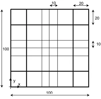
The original global model consists of two-dimensional shell elements of first order and one-dimensional bar elements, also of first order, used as stiffeners. A 3D representation of the generic model is shown in Figure 3.1. However; note that the figure is only a representation and does not show the true dimensions, see Figure 3.2 and Figure 3.3 for dimensions of the global model and beams. The global coordinate system is defined with origin in the lower left corner.
The width of the global generic model is 100 mm, height 100 mm and the thickness of the shell elements is 2 mm. As seen in Figure 3.1, the global model consists of 6 times 6 elements, however the element size of the shell element is not uniform; the standard size is 20 times 20 mm whereas the side centred regions are split into two equally sized elements and the central region is split into 4 equally sized elements. The four central elements are later replaced by the local model. The
dimensions of the global model are seen in Figure 3.2.
Figure 3.2: Dimensions and coordinate system of the global generic model. Beams are represented with thick lines. Dimensions in mm
The beams are placed on the boundary of the plate and 20 mm from the boundary parallel to it. The beams are T-shaped with dimensions according to Figure 3.3. The properties for the beams are stated in Table 3.1, the material is the same as for the shell elements described in Table 3.2.
2 2 3 5 100 100 20 20 x y 10 10
Table 3.1: Beam properties for generic model
Property Value Unit
Area A 16 mm2
Inertia 1,1 Iy 22.8 mm4
Inertia 1,2 Ix 31.3 mm4
3.1.1 Material
The entire global model is built of aluminium, which is a commonly used material for aircrafts. It is defined as a linear elastic and isotropic material with properties stated in Table 3.2. The same material data is used for all local models.
Table 3.2: Material properties of aluminium for the generic model
Property Value Unit
Elastic Modulus E 71800 MPa
Poissons ratio 0.33 - Shear Modulus G 27000 MPa
3.2 The Local Models
The four central elements in the global model are replaced by a local model with a more refined mesh. To test the ability of the different Global-Local modelling techniques, different types of local models are used. Since the mesh of the local model in a real case scenario almost never is in contact with the global models at all nodes, some test cases are preformed where gaps and offset are present.
All local models are built of aluminium, with same material properties as in the global model. A summary of all cases of local models is found in Table 3.3.
Table 3.3: Summary of local model cases. *Number of element and the element sizes for case 3 and
4 is different for different sub-cases, see respectively section for more information Case no Element type Number of Elements Element size [mm] Offset
1 Shell 100 2*2 No
2 Solid 100 2*2*2 No
3 Shell 100 or 90* 2*2* Yes
4 Solid 100 or 90* 2*2*2* Yes
Case 1 and 2 test the methods for compatible geometry with shell and solid elements respectively, and case 3 and 4 test the methods when the geometry have offsets and gaps with shell and solid elements respectively..
3.2.1 Case 1: Shell Elements
The first and most basic local model consists of 10 times 10 shell elements that each has a width of 2 mm, height of 2 mm and a thickness of 2 mm. The outer corner nodes and side-centred nodes are equivalent to the nodes in the global model. The local model is illustrated in Figure 3.4.
Figure 3.4: Local model (green) for Case 1, consisting of 100 shell elements
3.2.2 Case 2: Solid Elements
The second local model has the same number of elements as in case 1, but here they are solid elements with the same dimension as before. The local model for Case 2 is shown in Figure 3.5. The solid elements are centred on shell elements, meaning that 1 mm is above the mean surface of the shell elements and 1 mm is below.
3.2.3 Case 3: Offset With Shell Elements
Case 3 is divided into several sub-cases, testing how the method can deal with offsets and non-cohesive geometry. All sub-cases are summarized in Table 3.4 and they are all based on the geometry from case 1. The local model consists of shell elements.
Table 3.4: Summary of sub-cases for offset with shell elements
Number of elements Gap relative global model [mm] Case no Element size [mm]
x y z x=40 x=60 y=40 y=60 z=0 3a Uniform 2.2 9 10 - 0 2 0 0 0 3b Uniform 2.2 9 10 - 1 1 0 0 0 3c Uniform 2.2 10 10 - 0 0 0 0 0.1 3d Variable 10 10 - 0 0-1.9 0 0 0 3e Variable 10 10 - 0 0.1 0 0 0 3f Variable 10 10 - 0 0.01 0 0 0 3g Variable 10 10 - 0 0.001 0 0 0
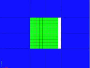
In Cases a-b 10 elements are removed of the local model, see Figure 3.6 and Figure 3.7. Case c only has an offset in z-direction, see Figure 3.8. Cases d-g all have 100 element but with variable sizes; in Case d, the 10 elements along the right side are transformed according to Figure 3.9, and in Cases e-f are the outer nodes along the right side moved in negative x-direction according to distances stated in Table 3.4, see Figure 3.10.
Figure 3.6: Geometry for local generic model (green) for Case 3a (shell elements) and 4a (solid elements). The gap, on the right side of the local model is 2 mm
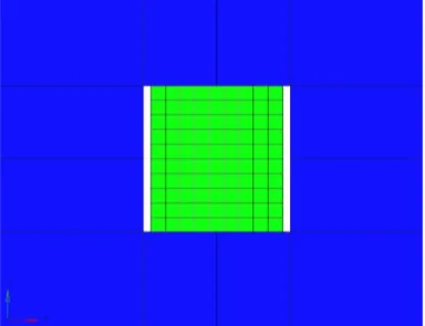
Figure 3.7: Geometry for local generic model (green) for Case 3b (shell elements) and 4b (solid elements). The gap to the global model is 1 mm on both left and right side
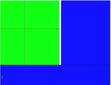
Figure 3.8: Geometry for local generic model (green) for Case 3c (shell elements) and 4c (solid elements). The entire local model has an offset in z-direction
Figure 3.9: Geometry for local generic model (green) for Case 3d (shell elements) and 4d (solid elements). The gap, on the right side of the local model is 0 mm in the top and 1.9 mm in the
bottom
Figure 3.10: Zoom of geometry for local generic model (green) for Case 3e-g (shell elements) and 4e-g (solid elements). The gap, on the right side, to the global model is 0.1, 0.01 respectively 0.001
mm
3.2.4 Case 4: Offset With Solid Elements
Case 4 is, as Case 3, also divided into several sub-cases, the difference is however that Case 4 uses a local model consisting of solid elements, with geometries based on Case 3, and another magnitude of the offset for Case 4c. All sub-cases are summarized in Table 3.5.
Table 3.5: Summary of sub-cases for offset with shell elements
Number of elements Gap relative global model [mm] Case no Element size [mm]
x y z x=40 x=60 y=40 y=60 z=0 4a Uniform 2.2 9 10 1 0 2 0 0 0 4b Uniform 2.2 9 10 1 1 1 0 0 0 4c Uniform 2.2 10 10 1 0 0 0 0 0.5 4d Variable 10 10 1 0 0-1.9 0 0 0 4e Variable 10 10 1 0 0.1 0 0 0 4f Variable 10 10 1 0 0.01 0 0 0 4g Variable 10 10 1 0 0.001 0 0 0
3.3 Reference model
For comparison of the results, all cases of local models for the tested methods are compared to a reference model. The reference model consists of shell and beam elements with the size 2 times 2 mm according to Figure 3.11.
Figure 3.11: 3D representation of the reference model
3.4 Load Cases and Boundary Conditions
Four different load cases are tested for all types of local models, where the loads for the first three load cases are applied consistent equally large on each node on the upper boundary (y-max), except the middle node. However, note that the load cases are not applied consistent over the geometry; the
The load cases are all small fictive values. All load cases and their corresponding boundary conditions are described in detail in Table 3.6. Common to all load cases is that all nodes on the lower boundary (y-min) are fixed.
The load cases are used on all test cases for the generic model and also on a reference model with a dense mesh.
Table 3.6: Load cases and their boundary conditions. Upper nodes are the nodes at y=100 except [50, 100, 0], lower nodes are all nodes at y=0, the central node is placed at [50, 50, 0] for shell
models and [50, 50, 1] and [50, 50, -1] for solid models (half load in each node)
Name Type of Load Magnitude and Direction per Node Unit Boundary Condition
Force_x Force, upper nodes [10, 0, 0] N Fixed, lower nodes Force_y Force, upper nodes [0, -10, 0] N Fixed, lower nodes Force_z Force, upper nodes [0, 0, 10] N Fixed, lower nodes Central_y Force, the central node [0, -50, 0] N Fixed, lower nodes
a) Force_x b) Force_y
Figure 3.12: Definition of load case Force_x and Force_y
a) Force_z b) Central_y
3.5 Evaluation of the results
The results are interpreted and evaluated in three steps. Partly visually based on results plots of the displacement and stresses but also from diagrams of the displacements and stresses along a given line in the centre of the model. Depending on the load case, different stresses are studied. For Force_x the shear stress is studied and for Force_y as well as Central_y the normal stress in the y-direction is studied. For all these load cases, the stress values are extracted from the mid-plane, which is the average of the top and bottom side of the element. Since Force_z causes a bending moment, the stress in the mid-plane will be zero or close to zero, therefore; the stress in the y-direction on the top surface of the shell is studied. The y-directions of the stresses are chosen with respect to which direction has felt the largest impact for each of the load cases. The displacements are studied in the same direction as the applied load.
To interpret the results, a few evaluation criteria are used; the quality of the connection, the accuracy of the displacement results and the accuracy of the stress results compared to reference values. Each evaluation criterion gives a score between 0 and 1, where 0 is a very poor result and 1 is total consistency with the reference values. The scores from each criterion are then weighted to an overall total score.
3.5.1 Evaluation Criterion 1 - Connection
The first step of the evaluation is to investigate whether the connection between the two models works properly. For Glue, it is possible to plot the nodes that are glued to each other, see the example in Figure 3.14; it is also possible to look at reaction forces at the boundary between the models, to see that there is a connection. Furthermore, the quality of the connection may be studied with use of displacement plots, where it is possible to see how the model is bending due to the force applied. If there are large gaps between the models the quality of the connection is poor and should usually not be approved. However, for some methods it is impossible to completely remove all gaps due to that the distance between the coupled nodes can be large, but the boundary of the local model should still have approximately the same displacement as the global boundary.
This criterion will give a score of either 1, 0.5 or 0. If there is a properly working connection the score will be 1, if there is a working connection but with large gaps or other defects, the score will be 0.5 and finally, the score is 0 if the method fails to connect the two models.
3.5.2 Evaluation Criterion 2 – Displacements
The second evaluation criterion is to look at the displacement results at a given line, Figure 3.15. The line goes through the entire model, both the global and local area.
Figure 3.15: Lines along which node displacements and stresses are extracted
The displacement results are extracted from the nodes at the middle line in the same direction as the applied load, for example; the displacement results for the x-component are extracted for the load case Force_x. The reference system used is the global system, and when solid elements are present, the average displacement is calculated between the top and bottom node for a given x-position to produce results in the mid-plane.
The results are exported to Excel where data files are created which are then read in MATLAB where plots and criterion scores are calculated according to the formulas stated in Section 3.5.4 below. The criterion score is calculated only from values within the local area. To be able to ignore the boundary effects, the two outer elements on each side of the local model are not evaluated.
3.5.3 Evaluation Criterion 3 – Stresses
The third evaluation criterion looks at the stress results at the same line as for the second criterion. As before, the line goes through the entire model, both the global and local area.
The stress results are extracted from the nodes at the middle line. The direction of the extracted stress depends on the load case, discussed above. The reference system used is the global system, and all results are extracted from the middle plane of the elements, except for load case Force_z
Middle line at y=50
The results are exported to Excel where data files are created which are then read in MATLAB where plots and criterion scores are calculated according the formulas stated in Section 3.5.4 below. The criterion score is calculated only from values within the local area. To be able to ignore the boundary effects, the two outer elements on each side of the local model are not evaluated.
3.5.4 Calculations of Individually Criterion Scores
Two different criterion scores are calculated for the displacement and the stress results respectively, which are then merged into one combined score for each evaluation criterion, m, and case, n. The method is influenced by Hovenga (2005), and is implemented in MATLAB according the code stated in Appendix A - MATLAB Script for Evaluation of the Parametric Study. The first criterion score-array is calculated with the Relative Error Method (REM), according to Equation 3.1, for values between x=44 and x=56. The choice of evaluated area is based on results from contour plots and on the fact that boundary effects will always be present. The error is therefore calculated for the local model except for the two outer elements on each side. The array for REM is plotted against the x-position and the lowest score is chosen as the Relative Error criterion score for the studied case.
56 44 , , ,
)
(
min
)
(
)
(
)
(
1
,
0
max
)
(
x x n REM n REM n n n n REMx
crit
CRIT
x
reference
x
case
x
reference
x
crit
(3.1)The Relative Error Method is not associative, meaning that the results differ if the reference is compared to the case instead of the opposite;
crit
REM(
ref
,
case
)
crit
REM(
case
,
ref
)
. Therefore, the Relative Error Method tends to under predict some cases and a second method is introduced, the Factor Method (FM), explained in Equation 3.2. The array is also here plotted against the x-position between x=44 and x=56 and the lowest score is chosen as the factor criterion score for the studied case.56 44 , , 2 2 ,
)
(
min
)
(
,
)
(
max
)
(
)
(
,
0
max
)
(
x x n FM n FM n n n n n FMx
crit
CRIT
x
case
x
reference
x
case
x
reference
x
crit
(3.2)The Factor Method is, unlike the Relative Error Method, associative;
)
,
(
)
,
(
ref
case
crit
case
ref
crit
FM FM .The two criteria scores are merged to a combined score with a weight factor of
w
1
2
for each criterion method, according to Equation 3.3, where j represents the two different criterion methods,56 44 , , , ,
)
(
min
)
(
)
(
x x n comb n comb j n j j n combx
crit
CRIT
w
x
crit
w
x
crit
(3.3)Finally, the array for the combined score is plotted against the x-position between x=44 and x=56 and the lowest score is chosen as the combined criterion score for the evaluation criterion and studied case.
3.5.5 Total Criterion Score
A total criterion score is calculated from the criterion scores from each evaluation criteria,
according to equation 3.4, where m represents the three evaluation criterions and n the studied case.
m n m comb m n total
W
CRIT
W
CRIT
, , , (3.4)However, if the first evaluation criterion score is 0, the total criterion score will also be set to 0. The weight factors for the criterion are summarized in Table 3.1. Since the first evaluation criterion is not that detailed, the weight factor is smaller than for the other evaluation criteria and is set to half of the weight factor for the second and third criterion.
Table 3.7: Weight factors for evaluation criterion Criterion number Weight factor, W
1 - Connection
1
5
2 - Displacements2
5
3 - Stresses2
5
3.5.6 Approved Results
For an overall approved result, the fist criterion has to be greater or equal to 0.5, the second and third criterion have to have a score of at least 0.8 or higher, and finally, the total score has to be at least 0.9 or higher.
The score for the second and third criteria are both in average 0.82 for the coarse global model, and the total score is in average 0.86 for the same model. The limits for approved results on the tested models are chosen after consideration with staff at Saab with respect to the values for the global model. The limits should not punish the individual criteria so hard, but the total score has to be
CHAPTER 4
PARAMETRIC STUDY
This chapter describes the parametric study performed on the generic model described in previous chapter. The choice of which methods to implement is based on available software, which methods that have not been used on Gripen before, requests from Saab and time aspects. The results and outcome from the simulations are presented here. The results are evaluated with three different criteria described in previous chapter. A user guide to all used methods is found in Appendix D User Guide to Used Methods. The individual, combined and total criteria scores are found in Appendix B Results from Parametric Study.
4.1 Reference Values
All load cases are applied to the reference model with 2 times 2 mm large shell and beam elements. These results are used as reference values to compare the results from each case with, when evaluating the simulations done for the different techniques. The maximum and minimum stresses and the displacements for all load cases can be found in Table 4.1.
Table 4.1: Summary of stresses and displacement for the reference generic model. Displacements are defined in the same direction as the applied force. Stresses looked at: Force_x – yx , mid-plane;
Force_y – y, mid-plane; Force_z – y, top plane and Central_y – y, mid-plane. Force_x Force_y Force_z Central_y
Min stress [MPa] 3.60e-2 -8.69e-1 -1.15 -2.57 Max stress [MPa] 4.37e-1 -1-95e-2 2.75e1 2.28 Min displacement [mm] 0 -4.80e-4 0 -5.93e-4 Max displacement [mm] 2.49e-3 0 7.50e-1 0
a) Displacement x-direction b) Stress xy, mid-plane
Figure 4.1: Results from the reference generic model for load case Force_x
a) Displacement y-direction b) Stress y, mid-plane
Figure 4.2: Results from the reference generic model for load case Force_y
a) Displacements y-direction b) Stress y, mid-plane
Figure 4.4: Results from the reference generic model for load case Central_y
4.1.1 Displacement Diagrams
All cases of the evaluated methods are numerically compared to the reference model, but in the displacement diagrams, results from the coarse global model are also included for the understanding of the appearance outside the local model. The goal is to achieve results that follows the global results outside the local model, but are closer to the reference model in the local area. The reference values are shown in Figure 4.5 to Figure 4.6.
a) Force_x b) Force_y
a) Force_z b) Central_y
Figure 4.6: Reference values for displacement results, Force_z and Central_y
4.1.2 Stress Diagram
As for the displacement criterion, all cases of the evaluated methods are numerically compared to the reference model, but in the stress diagrams, results from the coarse global model are also included. The reference values are shown in Figure 4.7 to Figure 4.8.
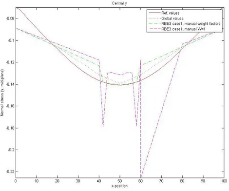
a) Force_x b) Force_y
a) Force_z b) Central_y
Figure 4.8: Reference values for stress results, Force_z and Central_y
4.2 Mesh Refinement
Mesh refinement is implemented for all load cases. The HyperWorks package is used where HyperMesh is the pre-processor, RADIOSS the solver and HyperView the post-processor. Due to the definition of the mesh refinement method, it is not possible to test different sub-cases with solid elements in the local area or with gaps or offsets. The used model is shown in Figure 4.9, and can be compared to Case 1 of the generic model, with 10 times 10 elements in the local area.
Figure 4.9: Model for test of Mesh refinement. Red lines represents bars with same properties and dimensions as for the generic model
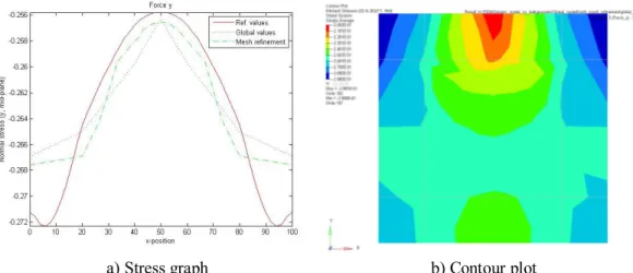
Figure 4.10 and Figure 4.11 show examples of the results from the displacement and stresses. The figures shows load case Force_y, but the other load cases have similar ratio to the reference values. The results from the mesh refinement test follows the values from the global model in the coarse
a) Displacement graph b) Contour plot
Figure 4.10: Displacement results from mesh refinement for load case Force_y
a) Stress graph b) Contour plot
Figure 4.11: Stress results from mesh refinement for load case Force_y
The combined criterion scores for mesh refinement are found in Table 4.2.
Table 4.2: Combined criterion scores of results for mesh refinement
Force_x Force_y Force_z Central_y
1 - Connection 1 1 1 1
2 - Displacements 0.97 1.00 1.00 0.96
2 - Stresses 0.98 1.00 1.00 0.99
Total score 0.98 1.00 1.00 0.98
4.3 RBE3
RBE3 elements are implemented as interface elements for all load cases. The HyperWorks package is used where HyperMesh is the pre-processor, RADIOSS the solver and HyperView the post-processor. The method used to define the interface elements is an automated Tcl-script provided by Altair. The nodes at the boundaries are defined and the script creates RBE3 elements to connect the models. The script is designed for Shell-To-Solid coupling which means that if a Shell-To-Shell coupling is used the properties of the RBE3 elements have to be modified or a new script could be constructed. For the tests performed here, the properties have been modified, see Appendix D User Guide to Used Methods, for the entire workflow. RBE3 is also available in other software but HyperWorks is used due to the automatic script that is available to simplify the implementation. The automated script is designed to make the local nodes independent (master) and the global nodes dependent (slave), meaning that the global nodes will follow the movement of the local nodes. This is not the traditional way to use RBE3 elements and therefore is some test performed were the RBE3 elements have been manually defined, were the local nodes are slaved to the global nodes, see Figure 4.12 for the difference in implementation. The automated method can have almost infinite numbers of master nodes connected to one slaved node, whereas the manual method have one or maximum two master nodes connected to one slave node. Due to time limitations of the project, these tests are only performed on Case 1 and Case 2, for all load cases. Figure 4.13 shows how the RBE3 elements have been defined around the local model for the different techniques.
a) Automated script b) Manually defined
Figure 4.12: Definitions of the RBE3 elements for the automated and manual methods. Master nodes are marked with a black triangle and slave nodes are marked with a white circle.
Another difference between the automated technique and the manually defined is the weight factors. The weight factors are default 1 in the automated script, meaning that the displacement in the slave node will be the average displacement of the master nodes, independent of the placement of the nodes. In the manually defined method, the weight factors are defined with respect to the geometry and placement of the nodes. For example, if the slave node is placed according to Figure 4.14, the contribution from node A is 1/3 and the contribution from node B is 2/3. The weight factors can be adjusted with a Tlc-script provided by Altair.
Figure 4.14: Definition of weight factors for manual method
Since RBE3 works independently of the size of the gap, all load cases will have a working connection. However since RBE3 does not have any stiffness the stiffness of the model will decrease, if gaps are present.
The results from all test cases for the automated method are summarized in Table 4.3. The results from the manually defined method are summarized in Table 4.4.
A B
l
l/3
Table 4.3: Summary of results for RBE3 automated method in HyperMesh. Load case approved?
Case no
Force_x Force_y Force_z Central_y
1 No No No No
2 Yes Yes No Yes
3a Yes Yes Yes No
3b Yes Yes Yes Yes
3c Yes Yes Yes Yes
3d Yes Yes Yes Yes
3e Yes Yes Yes Yes
3f Yes Yes Yes Yes
3g Yes Yes Yes Yes
4a Yes Yes No Yes
4b Yes Yes No No
4c Yes No No No
4d Yes Yes No Yes
4e No Yes No Yes
4f Yes Yes No Yes
4g Yes Yes No Yes
Table 4.4: Summary of results for RBE3 manually defined method in HyperMesh. Load case approved?
Case no
Force_x Force_y Force_z Central_y
1 Yes Yes Yes Yes
2 Yes Yes No Yes
4.3.1 Case 1: Shell Elements
For the automated methods, none of the load cases are approved, due to a bad matching of the stress values, however, the displacement values are almost identical to the reference model for most load cases. For the manually defined method, the stress values match the reference model much better and all load cases are in this case approved.
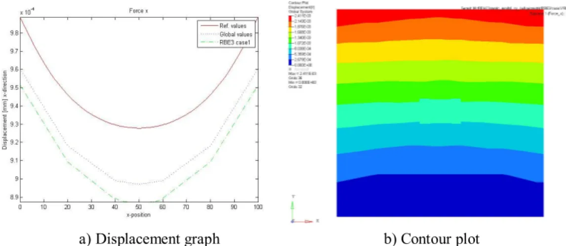
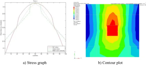
Figure 4.15 shows an example of how the displacement results look like for the automated RBE3 technique and load case Force_x. Figure 4.16 shows the corresponding stress results and Figure 4.17 shows the criteria scores for the displacement and stress criteria. It is here possible to see that the displacement follows the reference model quite good but the results for the stresses are worse. Due to the stress results, none of the load cases are approved.
a) Displacement graph b) Contour plot
Figure 4.15: Displacement results from RBE3 (automated) Case 1 for load case Force_x
a) Stress graph b) Contour plot