Forecast Performance Between SARIMA and SETAR Models: An Application to Ghana Inflation Rate

Forecast Performance Between SARIMA and SETAR Models:

An Application to Ghana Inflation Rate

Author

ERIC AIDOO

Supervisor

PROF. JOHAN LYHAGEN

i

Forecast Performance Between SARIMA and SETAR Models:

An Application to Ghana Inflation Rate

A dissertation submitted to the Department of Statistics, Uppsala University

in partial fulfillment of the requirement for the award of

Master of Science Degree in Statistics

By

AIDOO, ERIC

1

Supervisor

PROF. JOHAN LYHAGEN

JANUARY, 2011

ii

ACKNOWLEDGEMENT

(Showing gratitude paves way for future assistance)

The completion of this research has been possible through the help of many individuals who supported me in the different stages of this study. I would like to express my deepest appreciation to my supervisor Prof. Johan Lyhagen. Who despite his heavy schedule has rendered me immeasurable supports by reviewed the manuscript. His comments and suggestions immensely enriched the content of this work.

I am also grateful to all the lecturers and entire staffs of Uppsala University especially Dag Sörbom, Thommy Perlinger, Daniel Preve, and Niklas Bengtsson.

I have also benefited from the help of the many other individuals during my studies at Uppsala University, especially Timah Paul Nde, Kwame Duruye, Humphery Agbledeh, Baffoe Owusu Kwabena, George Adu, Gilbert Mbong, Amarfio Susana, Fransisca Mensah, Bernard Arhin and Emmanuel Atta Boadi.

Finally, I want to extend my sincere gratitude to officials of Ghana Statistical Service Department for their assistance in providing data for this exercise.

iii

DEDICATION

iv

ABSTRACT

In recent years, many research works such as Tiao and Tsay (1994), Stock and Watson (1999), Chen et al. (2001), Clements and Jeremy (2001), Marcellino (2002), Laurini and Vieira (2005) and others have described the dynamic features of many macroeconomic variables as nonlinear. Using the approach of Keenan (1985) and Tsay (1989) this study shown that Ghana inflation rates from January 1980 to December 2009 follow a threshold nonlinear process. In order to take into account the nonlinearity in the inflation rates we then apply a two regime nonlinear SETAR model to the inflation rates and then study both in-sample and out-of-sample forecast performance of this model by comparing it with the linear SARIMA model.

Based on the in-sample forecast assessment from the linear SARIMA and the nonlinear SETAR models, the forecast measure MAE and RMSE suggest that the nonlinear SETAR model outperform the linear SARIMA model. Also using multi-step-ahead forecast method we predicted and compared the out-of-sample forecast of the linear SARIMA and the nonlinear SETAR models over the forecast horizon of 12 months during the period of 2010:1 to 2010:12. From the results as suggested by MAE and RMSE, the forecast performance of the nonlinear SETAR models is superior to that of the linear SARIMA model in forecasting Ghana inflation rates.

Thought the nonlinear SETAR model is superior to the SARIMA model according to MAE and RMSE measure but using Diebold-Mariano test, we found no significant difference in their forecast accuracy for both in-sample and out-of-sample.

KEY WORDS: Ghana Inflation, SARIMA model, SETAR model, Forecast comparison, CH test, ZA test, KPSS test, HEGY test, Tsay test, Keenan test

v

TABLE OF CONTENTS

TITLE PAGE ... i ACKNOWLEDGEMENT... ii DEDICATION...iii ABSTRACT ... iv TABLE OF CONTENTS... v LIST OF TABLES ... vi

LIST OF FIGURES ... vii

1 INTRODUCTION... 1

2 MODELS AND METHODS ... 4

2.1 SARIMA Model... 4

2.1.1 Model Identification... 6

2.1.2 Parameter Estimation and Evaluation ... 15

2.1.3 Forecasting from Seasonal ARIMA model... 17

2.2 SETAR Model... 18

2.2.1 AR Specification and Linearity Test... 19

2.2.2 Model Identification... 22

2.2.3 Parameter Estimation and Evaluation ... 23

2.2.3 Forecasting from SETAR Model ... 24

2.3 Forecast Comparison... 25

3 DATA AND EMPIRICAL RESULTS ... 27

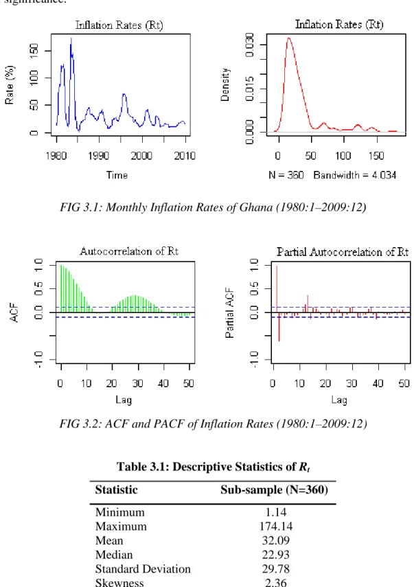
3.1 Descriptive Statistics... 27

3.2 SARIMA Modelling ... 29

3.2.1 Stationarity Test and Model Identification ... 29

3.2.2 Parameter Estimation and Evaluation ... 33

3.3 SETAR Modelling ... 36

3.3.1 Linearity Test ... 36

3.3.2 Model Identification... 37

3.3.2 Parameter Estimation and Evaluation ... 37

3.4 Forecast Comparison between SARIMA and SETAR Model... 36

4 CONCLUSIONS ... 42

vi

LIST OF TABLES

Table 2.1: Behaviour of ACF and PACF for Non-seasonal ARMA(p,q) ... 13

Table 2.2: Behaviour of ACF and PACF for Pure Seasonal ARMA(P,Q)s... 13

Table 3.1: Descriptive Statistics of Inflation Rates ... 28

Table 3.2: Unit Root Test for Inflation Rates... 30

Table 3.3: Unit Root Test for difference Inflation Rates ... 30

Table 3.4: HEGY Seasonal Unit Root Test for Yt... 31

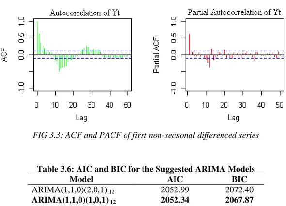
Table 3.5: CH Seasonal Unit Root Test of Y ... 31 t Table 3.6: AIC and BIC for the Suggested ARIMA Models ... 32

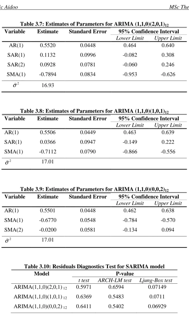
Table 3.7: Estimates of Parameters for ARIMA (1,1,0)(2,0,1)12... 34

Table 3.8: Estimates of Parameters for ARIMA (1,1,0)(1,0,1)12... 34

Table 3.9: Estimates of Parameters for ARIMA (1,1,0)(0,0,2)12... 34

Table 3.10: Residuals Diagnostics Test for SARIMA model ... 34

Table 3.11: Linearity Test ... 36

Table 3.12: AIC for the Suggested SETAR Models ... 38

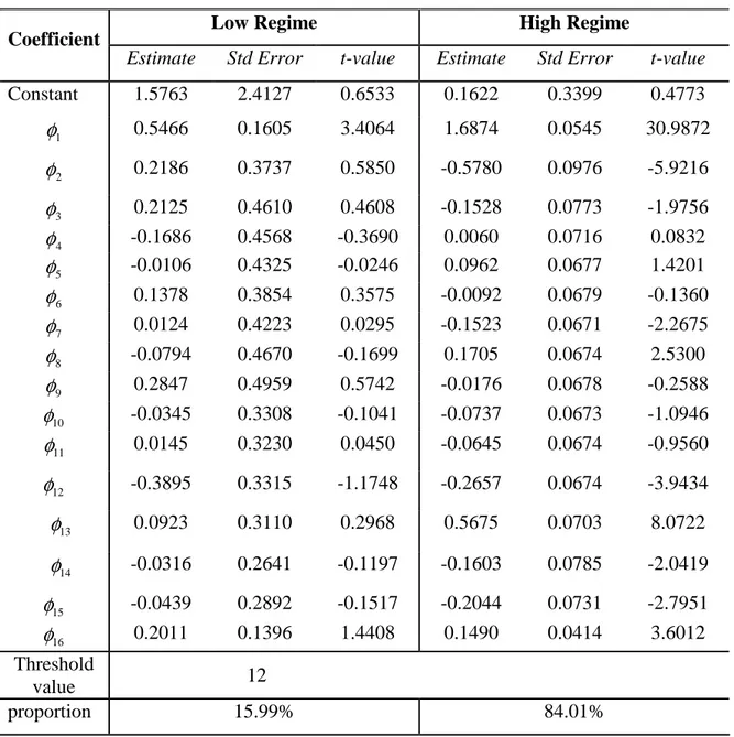
Table 3.13: Estimates of Parameters for SETAR (2;16,8) ... 38

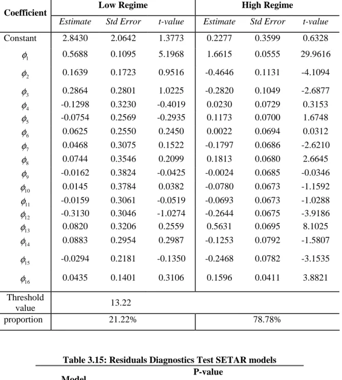
Table 3.14: Estimates of Parameters for SETAR(2;16,9) ... 39

Table 3.15: Residuals Diagnostics Test for SETAR models... 39

Table 3.16: Forecast Comparison among SARMA models ... 41

Table 3.17: Forecast Comparison among SETAR models ... 41

vii

LIST OF FIGURES

Figure 3.1: Monthly Inflation Rates of Ghana (1980:1–2009:12) ... 28

Figure 3.2: ACF and PACF of Inflation Rates (1980:1–2009:12)... 28

Figure 3.3: ACF and PACF of first non-seasonal differenced series... 31

1

1 INTRODUCTION

n recent years there has been an increase in both applied and theoretical research in time series modelling and forecasting. The research in this area has contributed to the success of several economies in the world. One of the economic variables that have received much attention in time series modelling is inflation. This is because inflation is one of the macroeconomic variables that have great impact in every economy and its forecasting has great importance for policy makers, investors, firms, traders as well as consumers. For instance, forecasting future inflation will enable policy makers to foresee ahead of time the requirement needed to design economic strategies to combat any expected or unexpected change in inflation. It will also enable investors, firms and others governmental and nongovernmental organisation to develop and evaluate economic policies and business strategies and also to take good decisions on their financial planning. Inflation is the major focus of economic policy worldwide as described by

David (2001). Inflation as defined by Webster (2000) is the persistent increase in the level of consumer prices or a persistent decline in the purchasing power of money. Inflation causes global concern because it can distort economic patterns when not anticipated. Inflation as described by Aidoo (2010) can cause uncertainty about the future price, interest rate, and exchange rate etc which as a result might increase the risk among potential traders and partners of a country.

In inflation modelling and forecasting, ARIMA class of models have been extensively used due to its ability in forecasting as compare to other linear time series models. The most commonly used model in the ARIMA class of models for inflation rates is the Seasonal Autoregressive Integrated Moving Average (SARIMA) model. For example, Aidan et al (1998) used SARIMA model to forecast Irish Inflation, Junttila (2001) applied SARIMA model approach in other to forecast finish inflation, and Pufnik and Kunovac (2006) applied SARIMA model to forecast short term inflation in Croatia,

Aidoo (2010) applied SARIMA models to forecast Ghana inflation rates etc. The SARIMA model is an extension of the ordinary ARIMA model proposed by Box and Jenkins (1976). This model is use to analyzes time series data which contain seasonal and non-seasonal behaviors. The models are also known to be good in modeling and

I

2 forecasting other macroeconomic time series such as unemployment rate and GDP. Due to the effect from business cycles, the dynamic features of inflation and other macroeconomic variables have been described as nonlinear by other research work such as Tiao and Tsay (1994), Stock and Watson (1999), Chen et al. (2001), Clements and Jeremy (2001), Marcellino (2002) etc. Laurini and Vieira (2005) argue that Brazilin inflation rate follows a nonlinear process. This means that the inflation and other macroeconomic variables display different features during economic expansion and recession. Hence, these variables have asymmetric properties which can not be captured by the simple linear models and also the forecast values based on this model may not be reliable. The required model to capture this asymmetric fluctuations or behaviour is the nonlinear times series models. An example of the nonlinear type of models includes the Self Excited Threshold Autoregressive (SETAR) model which is a special type of the TAR proposed by Tong (1978, 1983) and further discussed by Tong and Lim (1980), the Smooth Transitional Autoregressive (STAR) models proposed by Teräsvirta (1994), and the Markov Switching Autoregressive (MS-AR) models introduced by Hamilton (1989).

If the data generation follow a nonlinear process it is believed that a nonlinear model is suppose to perform better in terms of forecasting as compare to the linear model since it will be capable of handling the asymmetric features in the data. However as describe in some research the nonlinear models sometimes perform poor in forecasting as compare to the linear counterpart. In this we consider the Self Exited Threshold Autoregressive (SETAR) model.

In theoretical and applied research work of economic modelling the SETAR model have extensively been studied see Tong (1978, 1983), Tong and Lim (1980), Tiao and Tsay (1994), Potter (1995), Clements and Smith (1997), Rothman (1998), Clements and Krolzig (1998), Clements et al (1999), Feng and Liu (2002), Ismail and Isa (2006). The SETAR model is a set of different linear AR models, changing according to the value of the threshold variable(s) which is the past values of the series. The process is linear in each regime, but the movement from one regime to the other makes the entire process nonlinear. For some number of research work the model has proved to perform better as compare to other nonlinear models. For example, Feng and Liu (2002)

3 ARIMA model in forecasting the nonlinear Canadian real GDP data using two evaluation forecast techniques (multi-step and 1-step ahead forecast). They found out that the SETAR model performs better the ARIMA model in both in-sample and out-of-sample fit.

In this study, our main objective is to compare both in-sample and out-of-sample forecasting performance between linear SARIMA models and nonlinear SETAR model applied to monthly Ghana inflation rate, and to answer the question; Does Ghana inflation rates exhibit nonlinear behaviour? If so, do nonlinear models have superiority in forecasting Ghana inflation rates?

Also since there is limited amount of research concerning the application of SETAR model on inflation rate, we believed that this research will serve as a literature for other researchers who wish to embark on similar studies.

The study made use of monthly Ghana inflation rate from January 1980 to December 2010 which was obtained from the Statistical Service Department of Ghana. The study applied the SARMA and SETAR model following their modelling procedures in other to model the dynamics of Ghana inflation rates from 1980 to 2009. The remaining observations were used to access the out-of sample forecast performance from both models. After obtaining the forecast from both models, root mean squared error (RMSE) and mean absolute error (MAE), was employed to measure the accuracy of the forecasting from both models. A model with a minimum of these statistics was considered to be the best in terms of forecasting. Also the Diebold-Mariano test of forecast accuracy was used to test the significant difference between the forecast from both models

The structure of the remaining part of the paper is as follows: Section 2 introduces the SARIMA and SETAR models and describes the modeling cycles in each model. Section 3 also describes source and features of Ghana inflation rates and also illustrates how the theoretical methodology of both models were applied to model and forecast the inflation rates and also how the forecast performance between the two models were measured. Section 4 presents the concluding remarks.

4

2 MODELS AND METHODS

In this section we discuss the competing models used in this research work. The discussion begins by introducing the linear SARIMA model and the modelling cycle associated with the model. Then we consider the nonlinear SETAR model as well. The section also discussed how the two models will be compared to each other using forecast accuracy measure.

2.1 SARIMA Model

Seasonal AutoRegressive Integrated Moving Average (SARIMA) model is the generalization of the well known Box-Jenkins ARIMA model to accommodate a data with both seasonal and non-seasonal feature. The ARIMA model which is known to be a combination of the AutoRegressive (AR) and Moving Average (MA) models utilize past information of a given series in other to predict the future. The AR part of the model deals with the past observation of the series whiles the MA part deals with the past error of the series (see Hamilton, 1994; Pankratz, 1983). The ARIMA model is applied in the case where the series has no seasonal features and also differenced stationary. This means that an initial differencing is required for the data to be stationary. The ARIMA model with its order is usually presented as ARIMA (p,d,q) model where p, d, and q are integers greater than or equal to zero and refer to the order of the autoregressive, integrated, and moving average parts of the model respectively. The first parameter p refers to the number of autoregressive lags, the second parameter d refers to the order of integration that makes the data stationary, and the third parameter q gives the number of moving average lags (see Pankratz, 1983; Hurvich and Tsai, 1989; Hamilton, 1994; Kirchgässner and Wolters, 2007; Kleiber and Zeileis, 2008; Pfaff, 2008)

A process, {y is said to be ARIMA (p,d,q) if t} t d

y

∆ is described by a stationary ARMA(p,q) model. ∆ means differencing of y in d order to achieve stationarity. In _t general, we will write the ARIMA model as

5 where ε_t follows a white noise (WN) process. The autoregressive operator and moving average operator are defined as follows:

p pL L L L φ φ φ φ = − − 2 −L− 2 1 1 ) ( (2) q qL L L L θ θ θ θ = + + 2 +L+ 2 1 1 ) ( (3) 0 ) (L ≠

φ for φ <1, the process {y is stationary if and only if d=0, in which case it _t} reduces to an ARMA(p,q) process.

The generalization of ARIMA model to the SARIMA model occurs when the series contains both seasonal and non-seasonal behavior. This behavior of the series makes the ARIMA model inefficient to be applied to the series. This is because it may not be able to capture the behavior along the seasonal part of the series and therefore mislead to a wrong order selection for non-seasonal component. The SARIMA model is sometimes called the multiplicative seasonal autoregressive integrated moving average model and is denoted by ARIMA(p,d,q)(P,D,Q)S. This can be written in its lag form as

(Halim & Bisono, 2008):

t S t D S d S L L y L L L L θ ε φ( )Φ( )(1− ) (1− ) = ( )Θ( ) (4) p PL L L L φ φ φ φ = − − 2 −L− 2 1 1 ) ( (5) PS P S S S L L L L = −Φ −Φ − −Φ Φ 2 L 2 1 1 ) ( (6) q qL L L L θ θ θ θ = − − 2 −L− 2 1 1 ) ( (7) QS q S S S L L L L = −Θ −Θ − −Θ Θ 2 L 2 1 1 ) ( (8) where,

p, d and q are the order of non-seasonal AR, differencing and MA respectively. P, D and Q is the order of seasonal AR, differencing and MA respectively. yt represent observable time series data at period t.

ε_t represent white noise1 error (random shock) at period t. L represent backward shift operator (Lky_t = y_t−k)

S represent seasonal order (e.g.s=4 for quarterly data and s=12 for monthly data).

1

The error term is said to be white noise if has the following characteristics:

0 ) ( _t =

6 For effective model selection, there is a need to follow the model building stages suggested by Box-Jenkins. These model building stages includes model identification, parameter estimation and evaluation and then forecasting stage.

2.1.1 Model Identification

In the identification stage of model building steps, we determine the possible SARIMA models that best fit the data under consideration. But before the search of the possible model for the data, the data under consideration must satisfy the condition of stationarity. This is because the SARIMA model is appropriate for stationary time series data (i.e. the mean, variance, and autocorrelation are constant through time). If a time series is stationary then the mean of any major subset of the series does not differ significantly from the mean of any other major subset of the series. Also if a data series is stationary then the variance of any major subset of the series will differ from the variance of any other major subset only by chance (see Pankratz, 1983). The stationarity condition ensures that the properties of the estimated parameters from the model are standard. That is the t statistic will asymptotically follow the usual t distribution.

If this condition is assured then, the estimated model can be used for forecasting (see

Hamilton, 1994). To check for stationarity, we sometimes test for the existence or nonexistence of what we called unit root. Unit root test is performed to determine whether a stochastic or a deterministic trend is present in the series. If the roots of the characteristic equation (such as Equation 2) lie outside the unit circle, then the series is considered stationary1. This is equivalent to say that the coefficients of the estimated model are in absolute value is less than 1 (i.e. φ_i <1 fori=1,K,p_{). In testing for unit} root in a given series the features of the series must be known. When the series contains both seasonal and non-seasonal behaviour, the test of stationarity must be conducted on both components (seasonal and non-seasonal frequencies). In testing for stationarity under non-seasonal frequencies the most used approach is the one of Kwiatkowski et. al. (1992) and also Zivot and Andrews (1992).

7 Kwiatkowski-Phillips-Schmidt-Shin (KPSS) test proposed by Kwiatkowski et al. (1992) is an LM type test used to test the null hypothesis that a given observable series is level stationary and/or stationary1 around a deterministic trend. As describe in Pfaff (2008) the test take the null hypothesis as a stationary process against the alternative hypothesis of unit root process. The model considered in the test is given by (see Pfaff, 2008):

t t

t t r

y =ξ + +ε (9)

where r is a random walk, i.e. _t r_t =r_t−1 +u_t, and the error process u is assumed to be _t ) , 0 .( . .id _u2

i σ ; ξ_t is a deterministic trend; ε_t is also a stationary error. Ifξ =0, then this model is in terms of constant as deterministic regressor. The test statistics is constructed as either the series y is regress on only constant term (level) or constant term and _t deterministic trend (level and trend) depending on whether one wants to test level and/or trend stationary. Let the partial sum series of the residualsε)_tfrom the regression model be

∑

= = = t i i t t T S 1 . , , 2 , 1 , K ) ε (10)

Then the KPSS test statistic for the null hypothesis of stationarity is given by:

2 2 1 2 ε σ) T S LM T t t

∑

= = (11)

where σ)_ε2 is an estimate of the error variance of ε_t from the regression model. The optimal weighting function which correspond to the Bartlett window

1 1 ) , ( + − = l s l s w is

used as suggested by the authors to estimate the long-run varianceσ)_ε2; that is

∑

∑

∑

= = =+ − − + − − + = = T t l s T s t t t t l s T T l s 1 1 1 1 2 1 2 2 1 1 1 2 ) ( ε ε ε σε ) ) ) ) (12)

where l is the lag truncation parameter. In this exercise l =integer[4(_T/100)14].

The approximate upper tail critical values of the asymptotic distribution of the KPSS test are taken from Kwiatkowski et al. (1992).

1 _{For a given series}

t

8 As described by some research that some of the conventional unit root has low power against the null hypothesis and it is always advisable to use more that one test as discuss in Cheung and Chin (1997), Maddala and Kim (1998), Gabriel (2003) to obtained robust conclusion about the properties of the underling time series. For instance, Perron (1989) shown that the power of the ADF test has low power of rejecting the null hypothesis of unit root when there is break in the underling series. Engel (2000) warns

about the use of the KPSS because of its lack of power. Caner and Kilian (2001),

indicated that the KPSS tests show size distortions when the stochastic process is near to

non-stationarity. Chen (2002) also investigated the behaviour of the KPSS test in the

presence breaks and found that the test has power to reject the null hypothesis stationarity of the series in the presence of breaks. Otero and Smith (2003) also investigated the effect of the KPSS test in the presence of outlier and in their research they found that the power of the KPSS test to reject the null hypothesis of stationarity falls when the series has a unit root with outliers.

To avoid false conclusions the ZA test which is capable of handling data with breaks and also use different approach from the KPSS test can be employed.

Zivot and Andrews (ZA) test proposed by Zivot and Andrews (1992) is usually applied to test for stationarity of an observable series which is believed to have been affected by breaks. The test is sometime called a sequential break test. As discuss in

Perron (1989), if there is structural break in the observable series, the conventional unit root test such as ADF, KPSS, and PP test may reflect misspecification of the deterministic trend. So the ZA test which gives an alternative of the Perron (1989) test of unit root that assumes a known break point which is based on an exogenous phenomenon. With the ZA test the break points are endogenously determined within the model. The ZA test considers three different models in testing the null hypothesis of unit root against the alternative hypothesis of stationary with a one time break. The models considered in the test are given by (see Narayan, 2005; Harvie et. al, 2006; Waheed et. al 2006):

Model A

∑

= − − + + + ∆ + + = ∆ k j t j t j t t t c y t DU d y y 1 1 β γ ε α (13)

9 Model B

∑

= − − + + + ∆ + + = ∆ k j t j t j t t t c y t DT d y y 1 1 β θ ε α (14) Model C

∑

= − − + + + + ∆ + + = ∆ k j t j t j t t t t c y t DU DT d y y 1 1 β γ θ ε α (15)

where y_t represent the observable series with t =1,2,K,T, ∆ _{is the first difference} operator, ε_trepresent a white noise disturbance. Also DU_t represent an indicator dummy variable for a mean shift occurring at the break date (TB) whiles DT is an indicator dummy variable corresponding to the trend shift. The function of DU_t and DT is given by:    > = otherwise TB t if DU_t 0 1 and    − > = otherwise TB t if TB t DT_t 0

The ∆y_t−jterm in the model allows for serial correlation and ensures the disturbance term in the model is white noise. From above, Model A allows for a one-time change in the intercept, Model B allows for a one-time change in the trend, and Model C allows for one-time change in both the intercept and the trend.

According to Zivot and Andrew (1992), in the implementation of the ZA test the inclusion of the end points of the sample causes the asymptotic distribution of the statistics diverges to infinity. In this case some region must be chosen such that the end points of the sample are not included. The authors suggest that a trimming region be specified as (0.15T, 0.85T). The test consider all points as a potential candidate of break point but the final break point suggested by each model is selected recursively by choosing the value of TB for which the absolute value of the one-sided t-statistic for α is minimized. The critical values of the ZA test can be obtain from Zivot and Andrew (1992).

The stationarity under the seasonal frequencies can also be test to determine if the seasonal behaviour in the data is deterministic or stochastic. The most common approach is the one of Hylleberg et al (1990), see also Canova and Hansen (1995).

10 Hylleberg-Engle-Granger-Yoo (HEGY) test proposed by Hylleberg et al. (1990) is used to test the presence of seasonal unit root in an observable series. The test was first developed to apply to quarterly time series by the authors. The approach was extended by Franses (1990) to be applied to monthly time series. As discussed in Franses (1991) the seasonal differencing operator ∆₁₂will have 12 roots on the unit circle which can be decomposed as:

(

)(

)(

)(

)

(

)

[

]

[

(

)

]

(

)

[

]

[

(

)

]

(

)

[

]

[

(

)

]

(

)

[

1 3 2

]

[

1

(

3

)

2

]

, 2 3 1 2 3 1 2 3 1 2 3 1 2 3 1 2 3 1 1 1 1 1 1 12 B i B i x B i B i x B i B i x B i B i x iB iB B B B − + + − − − + + − − + − − + + + + − + − = − (16)

where all the terms other than

(

1−B

)

correspond to seasonal unit roots. Testing for unit roots in monthly time series is equivalent to testing for the significance of the parameters in the auxiliary regression presented below:

, ) ( * 2 , 7 12 1 , 7 11 2 , 6 10 1 , 6 9 2 , 5 8 1 , 5 7 2 , 4 , 6 1 , 4 5 2 , 3 4 1 , 3 3 1 , 2 2 1 , 1 1 , 8 t t t t t t t t t t t t t t t y y y y y y y y y y y y y B ε µ π π π π π π π π π π π π ϕ + + + + + + + + + + + + + = − − − − − − − − − − − − (17)

whereµ_t represent the deterministic part in the regression model consisting of a constant, 11 seasonal dummy variables or a trend. ϕ* B( )is a polynomial function of B for which the usual assumption applies and where

(

)

(

)(

)

(

)

(

)(

)

(

)(

)

(

)

(

)

(

)

(

)

(

)

(

)

(

)(

)(

)

(

)(

)(

)

(

)

. 12 , 8 2 4 2 4 , 7 2 4 2 4 , 6 4 2 2 4 , 5 4 2 2 4 , 4 8 4 2 , 3 8 4 2 , 2 8 4 2 , 1 1 , 1 1 1 , 1 1 1 , 1 3 1 1 , 1 3 1 1 , 1 1 , 1 1 1 , 1 1 1 t t t t t t t t t t t t t t t t y B y y B B B B B y y B B B B B y y B B B B B y y B B B B B y y B B B y y B B B B y y B B B B y − = + + + − − − = + − + − − − = + + + + − − = + + + − − − = + + − − = + + + − − = + + + + =

11 The estimates of the πican be obtained by applying the ordinary least squares method.

Testing for the significance of the π_iterms implies testing for both seasonal and non-seasonal unit roots. The null hypothesis of unit roots is tested by t-test of the separateπ's. The test involves the use of one-sided t-test in testing for the null hypothesis of π₁ =0 and the null hypothesis of π₂ =0. The two-sided t-test are used in testing for the null hypothesis of =0,_i=3K12

i

π . The F-test is used in testing the null hypothesis that pairs

of π's are equal to zero simultaneously (e.g. π₃ =π₄ =0) as well as the joint test of π's

(π₃ =L=π₁₂ =0_{). There is no seasonal unit root if}

2

π through π₁₂ are significantly different from zero. If π1 =0, then the presence of non-seasonal unit root 1 can not be rejected. According to Franses (1991), pairs of the complex unit roots are conjugates, so roots are only present when pairs of π's are equal to zero simultaneously and also in the case of all ,_i=1,2K12

i

π are equal to zero, it is appropriate to apply the ∆₁₂ filter. The

critical values for t-tests of the separateπ's, and for F-tests of pairs ofπ's, as well as for a joint F-test of π₃ =L=π_{12 can be taking from Franses (1990).}

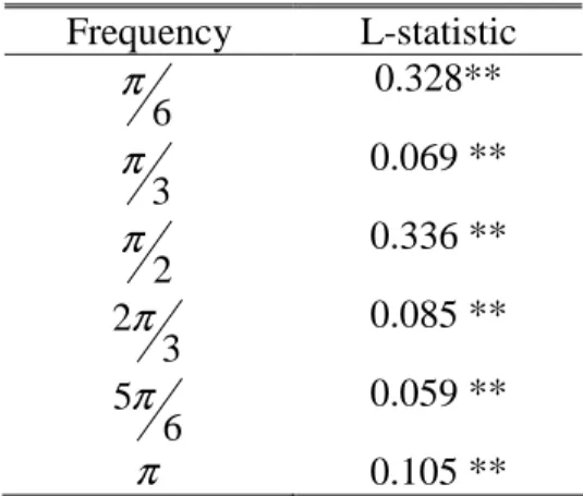
The Canova-Hansen (CH) test proposed by Canova and Hansen (1995) is one of the well known tests which are used to test for whether seasonality in observable time series is stochastic or deterministic. The test is usually considered as an extension of the KPSS test proposed by Kwiatkowski et al (1992) to test for null hypothesis of stationary seasonal against the alternative of seasonal unit root (non-stational due to seasonal unit root). As discussed in Caner (1998), the CH test statistics is a Lagrange Multiplier tests which include serially correlated and heteroscedastic processes. The autocorrelation in the process is handled by using a nonparametric adjustment. Given a regression model as in Banik and Silvapulle (1999):

yt xt dt et t 1,2, ,n

!

! + + = _K

= β α (18)

where y is the dependent variable, _t x is set of fixed regressors which includes and _t

intercept and/or linear trend, d is a set of deterministic seasonal component and _t e is a _t

white noise process. The CH test consider trigonometric representation of (18) as y_t =µ+x!_tβ+ f_t!γ +e_t (19)

12 where , , 1 1           =           = q qt t t f f f γ γ γ M

M _q=_{s/2 (s}=_{12 for monthly data),}

                  = q t j q t j

f_jt! cos π ,sin π for j<q and f_qt! =cos(πt).

In the test, in order to distinguish between non-stationarity at a seasonal frequency and at the zero frequency, it is require that y does not have a unit root at the zero frequency. If _t

t

y has a unit root at zero frequency then ∆yt = yt −yt−1is considered as dependent

variable (see Banik and Silvapulle, 1999).

In testing for unit root at a specific frequency, we rewrite (19) in such a way for individual seasonal frequency as:

∑

= + + + = q j t j jt t t x f e y 1 ! !β γ µ (20)

where γ jrepresent the seasonal cycle for the frequency (jπ/q).Hence test for a seasonal

unit root at frequency (jπ /q) reduces to testing for unit root in γ _j. Letting Ωf_jj

)

denote the jth block diagonal of Ωf

)

, the test statistic which is an LM test under the null hypothesis of stationary at the seasonal frequency (jπ/q)is given as:

∑

= − Ω = n t jt f jj jt q j F F n L 1 1 ! 2 ) / ( ( ) , 1 ) ) ) π (21) for j =1,2,K,q _where

∑

= = t i ji i jt f e F ₁ ) ) is the sub-vector of Ft ) partitioned conformably with γ. When the null hypothesis is satisfied, the distribution of L_(πj/q)is non-standard and the critical values are given in Canova and Hansen (1995).

According to Hylleberg (1995), the CH and the HEGY test complement each other. When the stationarity condition of the data is satisfied, the possible models suitable for the data can now be determined. The order of the model which AR, MA, SAR and SMA terms can be determine with the help of the ACF and the PACF plot of the stationary series. The ACF and PACF give more information about the behavior of the time series. The ACF gives information about the internal correlation between observations in a time series at different distances apart, usually expressed as a function

13 of the time lag between observations. These two plots suggest the model we should build. Checking the ACF and PACF plots, we should both look at the seasonal and non-seasonal lags. Usually the ACF and the PACF has spikes at lag k and cuts off after lag k at the non-seasonal level. Also the ACF and the PACF has spikes at lag ks and cuts off after lag ks at the seasonal level. The number of significant spikes suggests the order of the model. Table 2.1 and 2.2 below describes the behaviour of the ACF and PACF for both seasonal and the non-seasonal series (see Shumway and Stoffer, 2006).

Table 2.1: Behavior of ACF and PACF for Non-seasonal ARMA(p,q)

AR(p) MA(q) ARMA(p,q)

ACF Tails off at lag k

k=1,2,3,…..

Cuts off after lag q Tails off

PACF Cuts off after lag p Tails off at lags k

k=1,2,3,……

Tails off

Table 2.2: Behavior of ACF and PACF for Pure Seasonal ARMA(P,Q)S

AR(P)S MA(Q)S ARMA(P,Q)S

ACF Tails off at lag ks

k=1,2,3,…..

Cuts off after lag Qs Tails off at lag ks

PACF Cuts off after lag Ps Tails off at lags ks

k=1,2,3,……

Tails off at lag ks

The ACF and PACF plot suggest the possible models that can be obtained for the data but it does not give the final model for the data. This means that for a given series, several possible models can be obtained. In other to select the best model among the possible models, the penalty function statistics such as Akaike Information Criterion (AIC or AICc) or Bayesian Information Criterion (BIC) can be used (see Sakamoto et. al., 1986;

Akaike, 1974; and Schwarz 1978). The AIC, AICc and BIC are a measure of the goodness of fit of an estimated statistical model. Given a data set, several competing

14 models may be ranked according to their AIC, AICc or BIC with the one having the lowest information criterion value being the best. These information criterion judges a model by how close its fitted values tend to be to the true values, in terms of a certain expected value. The information criterion value assigned to a model is only meant to rank competing models1 and tell you which one is the best among the given alternatives. The criterion attempts to find the model that best explains the data with a minimum of free parameters but also includes a penalty that is an increasing function of the number of estimated parameters. This penalty discourages over fitting. In the general case, the AIC, AICc and BIC take the form as shown below:

      + − = n RSS n k or L k

AIC 2 2log( ) 2 log (22)

1 ) 1 ( 2 − − + + = k n k k AIC AICc (23) ) log( ) log( ) log( ) log( 2 2 n n k or n k L BIC=− + σ_e + (24) where

k = the number of parameters in the statistical model, (p+q+P+Q+1)

L = the maximized value of the likelihood function for the estimated model.

RSS = the residual sum of squares of the estimated model.

n = the number of observation, or equivalently, the sample size

2

e

σ = the error variance

The AICc is a modification of the AIC by Hurvich and Tsai (1989) and it is AIC with a second order correction for small sample sizes. Burnham & Anderson (1998) insist that since AICc converges to AIC as n gets large, AICc should be employed regardless of the sample size.

1 _{If two or more different models have the same or similar AIC or BIC values then the principles of}

parsimony can also be applied in order to select a good model. This principle states that a model with fewer parameters is usually better as compared to a complex model. Also some forecast accuracy test between the competing models can also help in making a decision on which model is the best.

15

2.1.2 Parameter Estimation and Evaluation

After identifying a possible model for the data, the next step in the model building procedure is to estimate the parameters of the selected model. The parameters are estimated using method of maximum likelihood estimation (MLE). At this stage we get precise estimates of the coefficients of the chosen model. That is we fit the chosen model to our time series data to get estimates of the coefficients. This stage provides some warning signals about the adequacy of our model. In particular, if the estimated coefficients do not satisfy certain mathematical inequality conditions1 that model is rejected.

After estimating the parameters of the chosen model, we then check the adequacy of that model which is usually called model diagnostics or model evaluation. Ideally, a model should extract all systematic information from the data. The part of the data unexplained by the model (i.e., the residuals) should be small as possible. The diagnostic check is used to determine the adequacy of the chosen model. These checks are usually based on the residuals of the model. One assumption of the SARIMA model is that, the residuals of the model should be white noise. If the assumption of are not fulfilled then different model for the series must be search for. A statistical tool such as Ljung-Box Q statistic, ARCH–LM test and t-test can be used to test the hypothesis of independence, constant variance and zero mean of the residuals respectively.

Ljung-Box statistic proposed by Ljung and Box (1978) is used to check if a given observable series is linearly independent. The test is usually used to check if there is higher-order serial correlation in the residuals of a given model. The null hypothesis of linearly independence of the series is examined by the test. The Ljung-Box test statistic is given by:

(

)

∑

= − + = h k k k T T T h Q 1 2 2 ) ( ρ ) (25) where

1 _{After the estimation of the parameters of the model, usually the assumptions based on the residuals of the}

fitted model are critically checked. The residuals are the difference between the observed value or the original observation and the estimate produced by the model. For the case of SARIMA model the assumption or the condition is that the residuals must follow a white noise process. If this assumption is not met, then necessary action must be taking.

16

k

ρ) = the sample autocorrelation at lag k T = the sample size

h = the number of time lags included in the test

When the null hypothesis is satisfied,Q(h) is asymptotically χ2 _{distributed with h}

degrees of freedom. The null hypothesis of linear independence is rejected if the

value

p− associated with Q(h)is small (p−value<α)or when the value of Q(h) is greater than the selected critical value of the chi-square distribution with h degrees of

freedom.

ARCH-LM test of Engle (1982) is used to check for conditional heteroscedasticity of the squared residuals a_t2 of a given model. Suppose a linear regression model given by;

, , , 1 , 2 2 1 1 0 2 T m t e a a a_t = + _t +K+ _{m t m} + _t = + K − − α α α (26)

where e denotes the error term, m is a prespecified positive integer, and T is the sample _t

size. According to Tsay (2005), the test for conditional heteroscedasticity which is also known as Arch effect is the Lagrange Multiplier test and is equivalent to the usual F

statistic for testing α_i =0(i=1,K,m) _{in the above Equation (26). The null hypothesis of}

no Arch effect in the squared residuals (i.e.α₁ =K=α_m =0)_{is examined by the test.}

Let

∑

+ = − = T m t t a SSR 1 2 2 0 ( ω) where

∑

=       = T t t a T 1 2 1

ω is the sample mean of a_t2, and

∑

+ = = T m t t e SSR 1 2 1 )

where e)_tis the least squares residual of the prior linear regression. The F

statistic as in Tsay (2005) is given by:

, ) 1 2 /( / ) ( 1 1 0 − − − = m T SSR m SSR SSR F (27)

When the null hypothesis is satisfied, F is asymptotically χ2(m)distributed with m

degrees of freedom. The null hypothesis of no Arch effect is rejected if the p−value

associated with F is small (p−value<α)or when the value of F is greater than the

17

2.1.3 Forecasting From Seasonal ARIMA Models

The last step in Box-Jenkins model building approach is Forecasting. After a model has passed the entire diagnostic test, it becomes adequate for forecasting. For exampleGiven Seasonal ARIMA (0,1,1)(1,0,1)12 model we can forecast the next step which is given by (see Cryer & Chan, 2008)

13 12 1 13 12 1 ( − − ) − − − − =Φ − + − −Θ + Θ − t t t t t t t t y y y y ε θε ε θ ε (28) 13 12 1 13 12 1 − − − − − − +Φ −Φ + − −Θ + Θ = t t t t t t t t y y y y ε θε ε θ ε (29)

The one step ahead forecast from the origin t is given by

12 11 12 11 1 − − − − + = t +Φ t −Φ t − t −Θ t + Θ t t y y y y) θε ε θ ε (30)

The next step is

11 10 11 10 1 2 = − − − − + = t +Φ t −Φ t −Θ t + Θ t t y y y y) ) ε θ ε (31)

and so forth. The noise terms ε₁₃,ε₁₂,ε₁₁,ε₁₀,K,ε_{1(as residuals) will enter into the} forecasts for lead times _l =1,2,K,13,_{but for l} >_{13 the autoregressive part of the model} takes over and we have

13 13 12 1 +Φ −Φ > = =− +− +− + y y y for l y)_{t l} )_{t l t l t l} (32)

18

2.2 SETAR Model

Self Excited Threshold Autoregressive (SETAR) model is a class of the Threshold Autoregressive (TAR) model proposed by Tong (1978) and further discussed in Tong and Lim (1980), Tong (1983, 1990). The SETAR model is a set of different linear AR models, changing according to the value of the threshold variable(s) which is the lagged values of the series. The process is linear in each regime, but the movement from one regime to the other makes the entire process nonlinear. The two regime version of the SETAR model of order p is given by (see Boero and Marrocu, 2004):

       > + + ≤ + + =

∑

∑

= − − = − − ) 2 ( ) 1 ( 1 ) 2 ( ) 2 ( ) 2 ( 0 1 ) 1 ( ) 1 ( ) 1 ( 0 p i d t t i t i p i d t t i t i t y if y y if y y τ ε φ φ τ ε φ φ (33) whereφi(1) and ) 2 ( i

φ are the coefficient in lower and higher regime respectively which needs to be estimated; τ is the threshold value; p and (1) p(2) are the order of the linear AR model in low and high regime respectively. In this work the order of the AR model in both regimes are equal. yt−d is the threshold variable that governs the transition between

the two regimes with d being the delay parameter which is a positive integer(d < p);

{ }

(1)

t

ε and

{ }

ε_t(2) are sequence of independently and identically distributed random variables with zero mean and constant variance (i.e. i.i.d.(0,σ_ε2) ). The two regime SETAR model in its simplest form can be written as SETAR (2, p, d). As discussed in

Tsay (2005), the properties of the general SETAR model are hard to obtain. Also from the discussion of Franses and van Dijk (2000), little is known about the condition under which the SETAR models generate time series that are stationary. Such condition has only been established for firs-order SETAR model. For effective model selection, we follow the procedure discussed in Franses and van Dijk (2000). The approach of SETAR modelling start with AR(p) model specification and linearity against SETAR model,

SEATR model identification, estimation and evaluation of the selected model and then forecasting.

19

2.2.1 AR Specification and Linearity Test

In order to apply the SETAR model to an observable time series, the series must first be nonlinear in nature. That is the existence of nonlinear behaviour in the series must first be checked. To test for nonlinearity in the series we first have specifies an appropriate linear AR(p) model for the series under consideration. As discuss in Franses and van Djik (2000), the choice of the maximum lag order is based on the autoregressive lag order that minimize the AIC value. After determine the linear AR(p) model we then test for

linearity using a well known linearity test such Keenan test and Tsay F-test.

Keenan test was introduced by Keenan (1985) to detect nonlinearity in an observable time series. The test is considered as a special case of the RESET test proposed by Ramsey (1969). It is a special case in the sense that it avoids multicollinearity. As describe in Cryer and Chan (2008), the Keenan test for nonlinearity analogous to Tukey’s one degree of freedom for nonadditivity test. As in Cryer and Chan, the Keenan test is motivated by approximating a nonlinear stationary time series by a second-order Volterra expansion which is give by:

∑

∑ ∑

∞ −∞ = ∞ −∞ = ∞ −∞ = − − − + + = u v u v t u t uv u t u t u y θ ε θ ε ε (34)

where

{

εt,−∞<t<∞

}

is a sequence of independent and identically distributed with

zero-mean random variable. The process

{ }

y is linear if the double sum of the right-hand side _t

of (34) does not exist. Thus we can test the linearity of the time series by testing whether or not the double sum of (34) does not exist. That is, the test requires that one distinguish between linearity versus a second-order Volterra expansion, by examining θuv =0 as well as the coefficients on higher orders.

It is shown in Cryer and Chan (2008) that the Keenan’s test is equivalent to testing if

0 =

η in the multiple regression model (with the constant 1 being absorb intoθ₀ ): yt =θ +φ yt− + +φmyt−m+ηyt +εt 2 1 1 0 ) K ₍₃₅₎

The Keenan’s test statistic for the null hypothesis of linearity (H₀ :η =0)is given as: ₂ 2 ) 2 2 ( η η − − − = RSS m n F ) (36)

20 where

m = lag order of the linear autoregressive process n = same size considered

RSS = the residual sum of squares from the AR(m) process

When the null hypothesis is satisfied, F

)

is approximately F-distributed1 with 1 and

2

2 −

− m

n degrees of freedom. The null hypothesis of linearity is rejected if the

value

p− associated with F

)

is small (p−value<α)or when the value of F

)

is greater than the selected critical value of the F-distribution with 1 and n−2m−2 degrees of freedom.

Tsay’s F-test introduced by Tsay (1989) is a test for detecting nonlinearity in an observable time series. The test considers a more general nonlinear alternative and is a combined version of the nonlinear test of Keenan (1985), Tsay (1986), and Petruccelli

and Davies (1986). According to the author the test is based on arranged autoregression

and predictive residuals. In the Tsay’s arranged regression approach, the linear AR(p)

model is considered in the null against the alternative hypothesis of nonlinear threshold model. For an AR(p) regression with n observation as yt =(1,yt−1,K,yt−p)β+at for

n p

t = +1 K, , where β is a (p+1)dimensional vector of coefficients and a is the _t

noise. The author refers to (yt,1,yt−1,K,yt−p)as a case of data for the AR(p) model. Then

an arranged autoregression is an autoregression with cases rearranged based on the values of a particular regressor. Consider a two regime TAR(2;p,d) model with n observations,

the threshold variable yt−d may assume values {yh,K,yn−d}, where }.

1 , 1

max{ p d

h= + − Let π_i be the time index of the ith smallest observation of

}. , ,

{y_h K y_{n−d Then the arranged autoregression with the first s cases in the first regime}

and the rest in the second regime is given by:

       > + Φ + Φ ≤ + Φ + Φ =

∑

∑

= + − + = + − + + p v d v d v p v d v d v d s i if a y s i if a y y i i i i i 1 ) 2 ( ) 2 ( ) 2 ( 0 1 ) 1 ( ) 1 ( ) 1 ( 0 π π π π π (37) 1 _F(1,n−_2m−₂₎

21 where s satisfies . 1 1 ≤ ₊ < _S S y

y_π τ _π The arranged autoregression provides a means by which

the observations are separated into two groups such that if the true model is indeed TAR(2;p,d) process, the observations in a group follow the same linear autoregressive model. According to the author the separation of the observation does not require knowing the precise value of τ1 and only the number of observation in each group

depends onτ₁. But since the threshold value is unknown, however the sequential least square estimates Φ(_v1)

)

are consistent for Φ(_v1) if there is sufficiently large number of observations in the first regime.

For the arranged autoregression, let β_m

)

be the vector of least squares estimates based on the first m cases, P the associated _m X'X inverse matrix, and x_m+1 the vector regressor of the next observation to enter the autoregression

1

+

+ m

d

y _π . Then the recursive least squares estimates can be computed efficiently by

_{1 1}[ ' ₁ ], 1 m m d m m m β K y _m x β β π ) ) ) + + + + = + + − (38) 1 ' 1 1 1.0 + + + = + m m m m x P x D , (39) K_m+1 =P_mx_m+1/D_m+1, and (40) m m m m m m P D x x P I P _      − = + + + + 1 ' 1 1 1 (41)

and the predictive and standardized predictive residuals is given by: a_d y_d x_{m m} m m π β π ) ) _' 1 1 1 + + + + = + − (42) and ed+π_m+1 =ad+π_m+1/ Dm+1 ) (43)

For fixed p and d, the effective number of observations in arranged autoregression is

. 1 + − −d h

n Assuming the recursive autoregressions begin with b observation so that

the there are n−d−b−p−hpredictive residuals available. We do the least squares regression

∑

= + − + + = + + p v d v d v d _{i i} i y e 1 0 π π π ω ω ε ) (44)

22 for i =b+1,K,n−d−h+1, _{and compute the associated F statistic under the null}

hypothesis of linear AR(p)

, ) /( ) 1 /( ) ( ) , ( ₂ 2 2

∑

∑

∑

− − − − + − = h p b d n p e d p F t t t ε ε ) ) ) ) (45)

where the ε)_t is the square residual of (44) and the argument (p,d)of F

)

is used to signify the dependence of the F-ratio on p and d. Suppose that y is a linear stationary t

autoregressive process of order p, then for large n the statistic F(p,d)

)

follows an asymptotic F distribution with p+1and n−d −b− p−h degrees of freedom.

The null hypothesis of linearity is rejected if the p−value associated with F(p,d)

)

is

small (p−value<α)or when the value of F(p,d)

)

is greater than the selected critical value of the F-distribution with p+1and n−d −b− p−h degrees of freedom

2.2.2 Model Identification

After the null hypothesis of linearity has been rejected we then select appropriate SETAR model that best fit the data. In this research we consider two regime SETAR model where the order p of AR model in both regimes are equal, that is SETAR(2;p,d). For a given

nonlinear time series, different SETAR models with different delay parameter d and

threshold value τ can be identified. The value of delay parameter is defined as the value for which the Tsay F statistic is significant and maximum. Also according to Tsay (1989)

the predictive residual can be used to locate the threshold values once the need for a threshold model is detected, see details from Franses and van Dijk (2000), Zivot and

Wang (2006). From all the possible models by a grid search the choice of the best model

can be selected based on the minimum of the usual information criterion which are the AIC and BIC. The AIC and BIC for the AR model in the two regimes as defined by Tong (1990) and presented in Franses and van Dijk (2000) is given by:

( , ) ln ln 2( 1 1) 2( 2 1) 2 2 2 2 1 1 2 1 p =n +n + p + + p + p AIC σ) σ) (46) BIC(p₁,p₂)=n₁lnσ)₁2 +n₂lnσ)₂2 +(p₁+1)lnn₁ +(p₂ +1)lnn₂ (47)

23 where 2 , 1 , j=

nj is the number of observations in the jth regimes and

2 , 1 , 2 = j j

σ) is the variance of the residuals in the jth regimes

1

p and p are the selected lag order in regime 1 and 2 respectively for which the 2

information criterion is minimized.

2.2.3 Parameter Estimation and Evaluation

After the desired model has been selected, the next step is to estimate the parameters of the selected model. The parameters can be estimated using a sequential conditional least square method. According to Franses and van Dijk, by using this method the resulting estimates are equivalent to maximum likelihood estimates (MLE) under the additional assumption that the residuals are normally distributed.

After the parameters of the selected model have been estimated, we then evaluate the adequacy of the selected model by accessing the residuals from the model which is usually called model diagnostics. The approach of access the adequacy of SETAR model may follow the same way as describe in section 2.1. As describe by Franses and van Dijk (2000), the usual ARCH-LM test and the t-test can be used to test the hypothesis of

constant variance and zero mean of the residuals respectively. But for the test of serial correlation the authors argue that the Ljung-Box statistic is invalid for the residuals from the nonlinear SETAR model and hence suggested the LM-type test proposed by Breusch- Godfrey.

The Breusch–Godfrey (BG) test proposed by Breusch (1979) and Godfrey (1978) is a Lagrange Multiplier test used to test for higher-order serial correlation in the residuals from a given regression model. Suppose a regression model given by:

yt =β0 +β1xt +ut (48)

where u is the OLS residuals from the regression model which might follow an _t

autoregressive process of order p which is given by:

u_t =α u_t− +α u_t− +L+α_pu_t−p +ε_t

2 2 1

24 The BG test uses the OLS estimation procedure to solve the auxiliary regression model given by: t p t p t t t t x u u u u) =β +β +α )₋ +α )₋ +L+α )₋ +ε 2 2 1 1 1 0 (50)

The test statistic for the null hypothesis (Ho :α1 =α2 =L=αp =0) is given by:

LM =TR2 (51)

where

T = the sample size

2

R = the usual coefficient of determination calculated from the model

When the null hypothesis is satisfied, LM is asymptotically χ2(p)distributed with p

degrees of freedom. The null hypothesis of no serial correlation of any order up to p is

rejected if the p−value associated with LM is small (p−value<α)or when the value of LM is greater than the selected critical value of the chi-square distribution with p

degrees of freedom.

2.2.4 Forecasting From SETAR Model

The important aim of considering nonlinear type of model such as SETAR as compare to the linear counterpart is to adequately describe the dynamic behaviour of the observable series under consideration and also to produce adequate forecast values that are far better than the one produced by the simple linear models. SETAR models have been successful been used to model and forecast a number of economic and financial data.

The optimal one step-ahead forecast from the origin t is given by (see, Franses and van Dijk, 2000):

y)_t+1|t =E[y_t+1|Ω_t]=F(x_t;φ) (52) where y)_t+1 is the forecast value for the time (t+1), and Ω_tis the history of the time series up to and including the observation at time t. F(x_t;φ)is the nonlinear function that represent the SETAR model. The next optimal step-ahead forecast is given by:

yt+2|t =E[yt+2 |Ωt]=E[F(xt+1;φ)|Ωt]

)

25 In general, the linear conditional expectation operator E can not be interchanged with the nonlinear operator F, that is

E[F(⋅)]≠F(E[⋅]) (54)

Put differently, the expected value of a nonlinear function is not equal to the function evaluated at the expected value of its argument. Hence,

E[F(y_t+1;φ)|Ω_t]≠F(E[y_t+1 |Ω_t];φ)=F(y)_t+1|t;φ) (55) The optimal h-step-ahead forecast can be obtained as

y)_t+h|t =E[y_t+h |Ω_t]=F(x_t+h−1;φ) (56)

2.3 FORECAST COMPARISON

In applied economic and financial modelling, the core point for estimating an econometric or time series model is so that the estimated model can be used to predict future value for decision making and policy evaluation. Forecasting is the process of making statements about events whose actual outcomes have not yet been observed. It is an important application of time series. If a suitable model for the data generation process (DGP) of a given time series has been found, it can be used for forecasting the future development of the variable under consideration. A good model for forecasting can be described as a model that produces minimum forecast errors as compare to other competing models. And to choose a final model for forecasting the accuracy of the model must be higher than that of all the competing models. The accuracy for each model can be checked to determine how the model performed in terms of both in-sample and out-of-sample forecast. Usually the model producing fewer out-of-out-of-sample forecast errors is preferred than a model producing fewer in-sample forecast errors. The forecast errors are the difference between the actual observations and the observations predicted by the estimated model. Usually in time series modelling some of the observations are left out during the model building process in other to access accuracy of the out-of-sample forecast of the estimated models. The accuracy of the models can be compared using forecast measure such as Mean Absolute Error (MAE), Root Mean Square Error

26 (RMSE). A model with a minimum of MAE or RMSE is considered to be the best for forecasting. In mathematical notation the MAE and RMSE are define as:

∑

∑

= = = − = T t t T t t t e T y y T MAE 1 1 1 1 ) (57)

∑

(

)

∑

( )

= = = − = T t t T t t t e T y y T RMSE 1 2 1 2 1 1 ) (58)

where y is the actual observation , t yt

)

is the forecasted value and T is the sample size.

The DM test proposed by Diebold-Mariano (1995) can also be used to check if there exist significant differences between the forecast accuracy of the two competing models. The null hypothesis of DM test is that there is no difference between the forecast accuracy from the two models against the alternative hypothesis that there is difference between the forecast accuracy from the two models. One sided test can also be performed.