The trade off between time and money : is there a difference between real and hypothetical choices?

(1)

The trade off between time and money:

Is there a difference between real and hypothetical choices?

Gunnar Isacsson

Swedish National Road and Transport Research Institute Transport Economics Research Unit

P.O. Box 760 S-781 27 Borlänge Sweden Phone. +46 243 44 68 67 Fax. +46 243 736 71 Email. gunnar.isacsson@vti.se

(2)

Abstract

This paper reports the results from one experiment and one quasi-experiment used to investigate the potential problem of “hypothetical bias” in surveys involving an individual’s valuation of time. The experiment compares hypothetical and real choices regarding an offer to participate in a survey in exchange for money. The quasi-experiment compares hypothetical and real choices regarding two bus journeys, one fast and expensive and the other slow and cheap. In both of these experiments, real choices differ significantly from hypothetical ones. The paper estimates parametric distributions of the value of time by applying the general method of moments (GMM) estimator. Since the samples are relatively small a parametric bootstrap is used to obtain asymptotic refinement of statistical tests. The results in the experiment as well as in the quasi-experiment suggest a value of time which is higher when the choice is for real than when the choice is hypothetical. Assuming that the value of time distribution is exponential, real choices produce a mean value of time twice as large as the corresponding hypothetical value.

(3)

1. INTRODUCTION

The value of time is among the most important factors in a cost benefit analysis of an investment in the transport infrastructure. Hensher and Brewer (2001, p. 85) note that the value of travel time savings usually account for some 70 percent of the user benefits in such analyses. This value is often estimated with data on hypothetical choices involving trade-offs between travel time and travel cost. Stated preference (SP) and the contingent valuation method (CVM) are leading methods for designing surveys involving hypothetical choices. There are some differences between the two methods. The CVM aims, for example, at valuing a specific good or a non-marginal change of a good, whereas SP aims at measuring how an individual values different attributes of a good; in other words, how the individual values marginal changes in attribute-levels. In addition, SP often entails repeated choices between different alternatives where the attributes of the alternatives are varied in a systematic way.1

Notwithstanding differences between CVM and SP, both of them rely on hypothetical choices and may consequently suffer from a “hypothetical bias”. Several studies have tested this problem in an experimental setting where individuals make both hypothetical and real choices.2 In a recent assessment of the literature on hypothetical bias Harrison (2006) concludes that “The most important finding from recent experimental work is that ‘hypothetical bias’ is an important and robust factor in valuation tasks, and is not reliably mitigated by varying basic elicitation procedures” (Harrison, 2006, p. 126). Usually hypothetically derived valuations tend to be higher than the corresponding real valuations.

Many of these experiments involve goods that are quite different from travel time, however; e.g. hunting permits and books. One difference between travel time and other goods is suggested by the additional time restrictions beside the conventional budget restriction in economic models of time allocation. Such additional constraints might imply that results from previous studies of hypothetical bias involving other goods are less informative with respect to hypothetically derived values of time. In fact, Brownstone and Small (2005) report that the

1

The SP-method comes under many different names and is sometimes called choice experiment or conjoint analysis. Some authors (for example Boxall et al., 1996) use the term “SP methods” for both the CVM and choice experiments. See Louviere et al, (2000) for a textbook introduction to SP methods.

2

See, for example, Bohm (1972), Bishop & Heberlein (1979), Brookshire and Coursey (1987), Neill et al. (1994), Cummings et al. (1995) and (1997), List & Shogren (1998), Frykblom (1998), Cummings and Taylor (1999), and Carlsson & Fredriksson (2001).

(4)

value of time estimated on real choices is some two times higher than that estimated on hypothetical choices. The sign of the hypothetical bias in the value of time would hence be of different sign than usually found for other goods. Their study pertains to faster express and reversible car pool lanes for which the drivers pay a toll upon usage. The authors interpret the difference between real and hypothetical choices as resulting from a scheduling constraint when individuals have not allowed sufficient time to choose the cheaper and slower alternative (Brownstone and Small, 2005, p. 288). Such constraints may be less obvious to an individual who indicates hypothetical choices between fast and expensive express lanes, and slow and cheap alternatives.

Smith and Mansfield (1998), on the other hand, find no significant differences between hypothetical and real choices in a field experiment regarding the value of time. As part of a telephone survey, they made respondents hypothetical and real offers to participate in another, future, survey in exchange for money. The offer did not, however, specify the exact time and date of the future survey. So the scheduling constraint discussed by Brownstone and Small (2005) is perhaps less pronounced in the study by Smith and Mansfield. Also, the future survey of Smith and Mansfield was never conducted due to a lack of resources.

The conflicting evidence and the few studies regarding hypothetical bias in studies of the value of time suggest the need for additional investigations of this issue. This is also the primary purpose of the present paper. It reports two tests of hypothetical choices applied to respondents’ valuation of time. In the first test all subjects started by filling in a survey questionnaire on their driving behavior. Subsequently, they were given an offer to fill in a second questionnaire concerning a similar kind of issue in exchange for money (the “survey experiment” for short in the following). A split random sample approach was used in this experiment. Thus, one group was given the offer for real; if they accepted the offer, they were paid a certain amount of money after completing the second questionnaire. The other group of subjects was given the offer hypothetically, meaning that they did not have to take any real consequences of their choices. In addition, individuals within each of the two groups were randomly given one of three distinct offers; that is, the amount of money offered varied between individuals. So a split random sample approach was also used within each of the two groups.

(5)

The second test is more adequately described as a quasi-experiment. In other words, it does not involve randomization of individuals into an experiment group and a control group as in the survey experiment. Instead the control group is selected so as to consist of individuals that are arguably similar to the individuals in the experiment group, both in terms of observed and unobserved characteristics. In this quasi-experiment, subjects were presented with a choice between two bus journeys where the time and cost of the two alternatives differed (“the bus experiment” for short in the following). One was fast and expensive and the other one was slow and cheap. One group of subjects made a choice where they actually had to use the chosen bus and pay the relevant amount of money, whereas another group merely indicated which bus they would have taken if the choice had been real. The main reason for not using a proper randomization was the small number of subjects that actually needed to use the bus.

The motivation for presenting both of these two tests of hypothetical bias is the relatively small sample sizes involved in each one of the two. In addition, the procedures of the two tests differ and the specific use of time is also different in the two tests. The comparison of the two tests also provides an assessment of whether randomization into an experiment group and a control group may be substituted for a matching procedure.3 As a secondary purpose of the paper, part of the econometric analyses aims at assessing whether potential differences between hypothetical and real choices is a result from a scheduling constraint as hypothesized by Brownstone and Small (2005).

The empirical framework of the present paper is somewhat different from previous investigations of hypothetical bias in the value of time. Instead of using a conventional random utility model, the paper tests for differences between real and hypothetical choices by directly comparing the value of time distributions in a framework similar to that suggested by Fosgerau (2006). More specifically, the paper tests for hypothetical bias both by comparing empirical cumulative distribution functions of the value of time, and by fitting parametric distributions to the observed choices. The latter involves an application of the generalized method of moments (GMM) estimator to relatively small samples. Since the GMM estimator may suffer from small sample bias, I also use the bootstrap to resample the empirical choice distributions to assess the small sample bias and to obtain asymptotic refinements of the t-test along the lines suggested by Hall and Horowitz (1996).

(6)

The paper is organized as follows. Section 2 presents a theoretical framework for the valuation of time. Section 3 outlines the experiments of the present paper. The results are presented in section 4. Section 5 concludes with a discussion of the results.

2. THE VALUE OF TIME

2.1 Theoretical framework

A useful theoretical point of departure for the valuation of time is the deSerpa (1971) model where the individual’s utility is defined over goods consumption (G), leisure (L) and time (T) spent in some kind of activity.4 Here this activity consists of filling in a questionnaire in exchange for money and spending time on a bus trip. Beside conventional budget- and time restrictions, the model also includes a time constraint related to T. In the present application assume that the individual solves:

) , , ( max , ,LTU u G L T G = (F1) s.t.

{

I P1,I P2 G∈ − −

}

(R1)

{

L1 +T1,L2 +T2 ∈ τ (R2)

where the index refers to one of two alternatives (1 and 2); R1 is the conventional budget restriction stating that total spending on real goods consumption must equal the difference between income (I) and the price of alternative 1 , or the difference between income and the price of alternative 2. R2 is the conventional time restriction that states that the total amount of time available

1

P

τ is divided between L and T. The individual either spends time in activity X and has leisure or spends in activity X and has leisure .

1 T 1 L T₂ L₂ 3

See Heckman and Hotz (1989) who suggest that experimental estimators of may be used to evaluate non-experimental estimators.

4

In the original deSerpa model there is a specific technical constraint related to T. Here this constraint is directly incorporated in R2.

(7)

The corresponding indirect utility function is

(

I Pi Ti Ti

u

V = − ,τ − ,

)

. (F2)

In empirical work a first-order Taylor expansion of the indirect utility function is often used; that is,

T P

V =α₀ +α₁ +α₂ (F3)

where the parameters for P and T measures the marginal utility of money and the marginal

disutility of time in activity X and the ratio 1 2

α α

is the value of time.

Thus, if the individual are faced with a choice between two distinct combinations of P and T: and , respectively, and is assumed to maximize utility (s)he will choose the alternative associated with the highest utility. In other words, if

(

P1, T1

)

(

P2,T2

)

2 2 2 1 1 2 1 1P α T α P α T α + > + , alternative 1 is chosen.

Introducing a scheduling constraint

Brownstone and Small (2005) hypothesize that differences between real and hypothetical choices result from a scheduling constraint that may be less obvious to respondents of a hypothetical survey even though they are pertinent to real choices. Suppose that alternative 2 is “slow and cheap” so that and . However, suppose that choosing the slow and cheap alternative comes at a cost beside . The individual may for example miss an important appointment by spending time rather in activity X. Let this cost be equal to C. Thus, the relevant choice to the individual is between the combinations

(

and

. If and it is clear that we cannot assess the trade off between 1 2 T T > P1 > P2 2 P 2 T T1

)

1 1, T P

(

P2 +C, T2

)

T2 >T1 P2 +C >P1

(8)

time and money since alternative 1 is better than alternative 2 both in terms of time and money. In other words, the individual will choose alternative 1 for sure. Note that C is unobserved to the analyst both in the hypothetical and real choice situation. The relevant question in the context of the present paper is to what extent individuals consider C in the hypothetical choice situation.

2.2 Empirical framework

There are different ways to take the model of section 2.1 to an empirical application. For example, adding a random error term to the indirect utility function (F3) to reflect unobserved heterogeneity leads to a conventional random utility framework within which we can estimate the two parameters of the indirect utility function.5 Fosgerau (2006) suggests instead that the population distribution of value of time be modelled directly. The average value of time in the population may then be estimated from the fitted distribution. Suppose for example that alternative 1 is fast and expensive and alternative 2 is slow and cheap, i.e. that and

. Thus, if an individual prefers alternative 2 to alternative 1 then his/her value of time (VoT) satisfies 2 1 P P > 1 2 T T > VoT =

(

)

(

1 2

)

2 1 1 2 T T P P − − − < α α

Hence, the share of individuals in a sample that prefers alternative 2 to alternative 1 gives us

an estimate of the cumulative distribution function at

(

)

(

1 2

)

2 1 T T P P − −

− . This ratio corresponds to a bid (b) in a willingness-to-pay (WTP) context or an offer in a willingness-to-accept, WTA, context. In the following I will refer to this as a ‘bid’ for short although ‘offer’ would be more adequate in the survey experiment. Fosgerau (2006) presents non-parametric, semi-parametric and parametric estimates of the value of time distribution. His results suggest, inter alia, that parametrically estimated mean values of time are very sensitive to the choice of distribution when the unobserved right tail of the distribution is fat.

5

To take a few examples, Truong and Hensher (1985), Smith and Mansfield (1998) and Brownstone and Small (2005) all use some kind of such a random utility model to estimate the value of time.

(9)

The results of the present paper are evaluated in a framework similar to that suggested by Fosgerau (2006). The samples of the present paper are relatively small, however. For this reason I only estimate the mean value of time parametrically, which implies that the level of the estimated mean values of time should be interpreted cautiously. The purpose of the present paper is, however, to see whether estimates of the value of time from hypothetical and real choices differ, so here the restrictions implicit in a parametric approach might be less problematic.

More specifically, the results of the experiment and the quasi-experiment are assessed in two ways. First, potential differences between real and hypothetical choices will be evaluated as differences between the cumulative distribution functions of real and hypothetical choices at the selected bids. The null hypothesis of no difference between real and hypothetical choices in the experiments is

( )

b F

( )

b F

H₀ : r = h

which is tested against the alternative

( )

b F

( )

b F

H_A : r ≠ h

where denotes the value of a cumulative distribution function at point b in the group

making real choices and the corresponding value in the group making hypothetical choices. The values of the two cumulative distribution functions at b are estimated by the share of individuals accepting the bid (b) in the real and the hypothetical treatment, respectively. Note that this test does not rely on a specific parametric cumulative distribution function.

( )

b Fr

( )

b Fh

The second way to assess the results is to estimate parametric distributions for the value of time from which it is possible to estimate the mean values in the real and hypothetical groups.6 To this end I apply the generalized method of moments (GMM) estimator to the following moment conditions:

6

(10)

( )

, 0 1 1 − = = −

∑

_μ b F y n m i n b b b , (M1)

where is the size of the sample receiving bid b (in the survey experiment of the present paper b=20, 60, or 100 and in the bus experiment b = 100 in terms of an hour) and

b n 1 = i y if

the bid is accepted by individual i (i=1,2, …, nb) and yi =0 if it is rejected and is a cumulative distribution function where b is the bid and μ is the parameter(s) of the distribution. Note that in the present case with a split sample approach may vary between different bids and hence between different moment conditions.

(

b,μ

F

)

b

n

In the present application M1 will be used to estimate two different cumulative distribution functions: the exponential distribution, and a mixture between the binomial and the exponential distribution. The motivation for choosing the exponential distribution is that the data from the bus experiment only allows identification of a one parameter distribution; i.e. there is only one moment condition. For ease of comparison of the bus experiment to the survey experiment the exponential distribution will also be fitted to the data from the latter.

The mixture will only be estimated on data from the survey experiment since it consists of two parameters. The motivation for choosing the mixture is to obtain an empirical model of the scheduling constraint outlined in section 2.1. Eye-balling the results also suggested that a mixture model might be reasonable (see section 4). To see why the mixture is relevant in the presence of a scheduling constraint, consider the case where there is a cost of choosing alternative 2 for some of the individuals. Assume that the cost C is sufficiently high so that

and . The fast and expensive alternative 1 is, thus, better than alternative 2 both in terms of time and money to these individuals. Clearly, an individual facing the cost C will always choose alternative 1 conditional on this set of prices. Let the probability that an individual do face the cost C, be 1-q. The mixture is thus

1 2 T T > P₂ +C >P₁

( )

(

1

)

exp 1 , =q − −bθ− b F μ ,

where θ is the mean value of time among individuals who do not face the cost C. Note that it is not possible to identify the corresponding mean for individuals facing the cost C. Hence, a

(11)

share (1-q) of individuals will choose alternative 1 for sure (with probability 1) whereas a share of individuals (q) chooses between alternative 1 and 2 along the ideas of section 2.1.

The purpose of estimating the mixture is thus to see whether the potential hypothetical bias results from differences in the indirect utility function (F3) or from differences in the estimated share (q) of individuals assumed to face the cost C. If the mixture would indicate a difference of the latter kind it would lend some support to the idea that scheduling constraints are relevant to the difference.

Note, furthermore, that there are three distinct bid levels in the survey experiment implying that there are two overidentifying restrictions when the estimated distribution is the exponential and one overidentifying restriction in the case of the mixture. One natural approach to using the moment restrictions efficiently is to apply the optimal (two-step) GMM suggested by Hansen (1982). However, there is evidence that the optimal GMM may be biased in small samples (see e.g. Altonji and Segal, 1996). To assess the magnitude of this bias I use the bootstrap to resample the empirical binomial choice distributions and obtain a bootstrap sample of estimates of in M1. The bias of the optimal GMM estimator may then be estimated by μ μ μˆb −ˆ where = −

∑

B₌ b b b B 1 1 ˆ ˆ μ

μ is the average of the bootstrapped estimates of taken over the number of bootstraps B, and μ is the estimate of obtained from the original sample. Thus, a bootstrap bias corrected estimate of is obtained by

μ

ˆ μ

μ b

biascor μ μ

μˆ =2ˆ − ˆ (see Cameron and Trivedi, 2005, p. 365, for a textbook treatment of bias reduction by the bootstrap).

The bootstrap has also been suggested as a means of obtaining asymptotic refinements of test statistics in finite samples (for an introduction see, for example, Horowitz, 2001). Since tests based on the GMM estimator have been shown to be quite misleading in finite samples, the bootstrap may be useful for obtaining asymptotic refinements of tests based on this estimator. Hall and Horowitz (1996) note, however, that the population moment conditions of the GMM estimator do not hold exactly in finite samples when the estimator is overidentified. In other

(12)

words, the moment conditions do not hold in the population from which the bootstrap samples. Hall and Horowitz (1996) therefore suggest applying the bootstrap on a recentered version of the population moment conditions. In the present context, this amounts to basing the bootstrap estimates of on μ

( )

, ˆ₂_, 0 1 1

∑

₋ ₋ ₌ = − b n j j b y F b m n b μ , (M2)

where and is the estimated parameters from the optimal two-step

GMM estimator applied to the original data, rather than on M1. All bootstrap estimates presented for the survey experiment are therefore based on M2 rather than on M1. The bootstrap will also be used to provide asymptotic refinements to the critical levels of the t-test applied to the difference between the estimated parameters in the real and hypothetical groups. Throughout I use 999 bootstrap replications. Appendix 1 contains a more detailed description of how the bootstrap GMM procedure is applied in the present paper.

(

2 1 1 , 2 ,ˆ ˆ n y F b μ m b n i i b b

∑

= − ₋ =

)

μˆ2 3. THE EXPERIMENTS

The basic idea of the two experiments reported here is, thus, to compare choices made in two groups of individuals, one where the choice is “hypothetical” and one where it is “real”. The individuals in the former group know that they do not have to take the consequences of their choice, whereas those in the latter group know that they must face the consequences of their choice.

(13)

3.1 The survey experiment7

Subjects were recruited among students during a lecture at Dalarna University (DU). Students were informed that they could participate in a survey that would take the last fifteen minutes of the lecture, and had two purposes: To investigate traffic behavior and economic decision making. After introducing students to the experiment, it proceeded by asking students who did not want to participate to step forward. No one did. Then, students without a driver’s license were asked to step forward. They were subsequently accompanied out of the class room.8 The remaining 135 students were randomly allocated to either the “real group” or the “hypothetical group”. The two groups were placed in two different rooms. No participation fee was used to recruit subjects for this experiment.

All subjects received a questionnaire on traffic behavior and a sealed envelope. They were given 15 minutes to complete the questionnaire. From the perspective of the experiment reported here, the purpose of the questionnaire was to make the subjects acquainted with the type of questionnaire they would later be offered to fill in exchange for money. Subsequently, they were told to open the envelope. The information in the envelope offered the subject to fill in a second questionnaire on a similar topic in exchange for money “here and now”. The subjects were informed that second questionnaire also would require 15 minutes to complete. The bid received by a particular subject was randomly determined to be either 5, 15 or 25 SEK which, thus, corresponds to a bid of 20, 60 or 100 SEK per hour.9 All kinds of communication were forbidden between subjects so that the all choices were made privately.

Subjects in the real group who accepted the offer filled in the second questionnaire and received the bid in cash after 15 minutes. Note that the 15 minutes required to fill in the second questionnaire pertained to 15 minutes after the lecture; subjects therefore traded time that was beyond the scheduled time of the lecture. Hence, scheduling constraints may be pertinent to the choices.

7

Appendix B contains an English version of the questionnaire that presented the choice to the subjects in this experiment.

8

Outside, they were informed that a requirement for participating in the experiment was to have a driver’s license and that hence, they were free to leave. The reason for restricting the sample to students with a driver’s license was simply that the questionnaire used in the experiment concerned driving behavior.

9

(14)

3.2 The bus experiment10

In this quasi-experiment, subjects were asked to choose between two alternative buses, one fast and expensive and one slow and cheap.11 Place of departure and arrival was the same for the two buses, but the slow and cheap bus had a different route than the fast and expensive one. The departure time of the former was therefore a quarter of an hour earlier than the latter. The arrival time was the same for both buses. The purpose of the journey was to take students DU to a series of three lectures with the title “writing for academic purposes”. DU is located in two towns, Borlänge and Falun, situated approximately 20 kilometers apart. The students participating in the experiment usually have their lectures in Borlänge, but in the experiment, they were instead given in Falun.

Subjects in the real group were among students who needed a transport to Falun. They were told that they had the opportunity to participate in an economic experiment where they would earn at least 100 SEK (the show-up fee). At the experiment, subjects were informed that they had a budget of 50 SEK besides the show-up fee, and were told to use this money to buy a ticket for either of the two buses. They were not informed in advance about the specific contents of the experiment, which was held some days before the actual journey.

Two hypothetical groups were recruited. One of them was recruited among students that would attend the lectures in Falun but who did not need transport. They were promised 100 SEK (the show-up fee) if participating in an economic experiment which was conducted some days before the lectures. The specific purpose of the journey was not described to these subjects and they did not receive any additional money beside the show-up fee. The other group was recruited among students who did not attend the lectures. They were also promised to earn at least 100 SEK if participating in a choice experiment. As opposed to the first hypothetical group, this group was informed about the specific purpose of the journey, and they were provided with an additional budget of 50 SEK upon arrival to the experiment. They were also told that if the choice had been real, the ticket cost would have been deducted from the 50 SEK.

10

Appendix C provides an English version of the questionnaire that presented the choice task to the subjects in this experiment.

11

(15)

All subjects were informed that they could choose one of two buses. The first bus would leave Borlänge at 8.15 a.m. and pass and stop in a small village located between Borlänge and Falun to pick up people there.12 The other bus would leave Borlänge at 8.30 a.m. and take the shortest route to Falun. Both buses would arrive just outside the university building in Falun at around 8.55 a.m., five minutes before the first lecture. The ticket cost was 25 SEK for the earlier bus and 50 SEK for the later one. Thus, the travel time and travel cost of the buses were 40 minutes and 25 SEK, and 25 minutes and 50 SEK, respectively; the bid is thus 100 SEK for an hour.13

Subjects were informed that all payments in the experiment were conditional on each subject actually traveling on the chosen bus. All payments were therefore made on the bus. Thus, a subject who had chosen “the fast and expensive bus” would be paid the show-up fee of 100 SEK on the bus, while a subject who had chosen the slow, low-cost bus would be paid the show-up fee plus the remaining part of the experimentally provided budget that is, in total 125 SEK. This provided an incentive for each subject to adhere to the chosen alternative and not to drop out of the experiment once the ticket had been bought.14

A corresponding experiment was conducted for the return journey where the slow, low-cost bus arrived a quarter of an hour later than the fast one to the destination (Borlänge). The experiment regarding the return journey took place during a break in between two of the lectures in Falun. This implies that some, but not all, subjects in the real and first hypothetical groups participated both in the experiment regarding the journey in the morning and the return journey in the middle of the day. The second hypothetical group was presented with both journeys in their experiment, however.

All kinds of communication were forbidden which ensured that all choices were made privately. This was achieved by letting them indicate their choice on a questionnaire. In the real group, subjects were subsequently given their chosen ticket.

12

An assistant in the experiment was actually waiting in the village and got on the bus as described to the subjects in the experiment. The intention was to avoid a situation where the real journey differed from the one described to the subjects.

13

(16)

4. DESCRIPTIVE STATISTICS AND RESULTS

4.1 The survey experiment

Table 1 presents descriptive statistics for the survey experiment. None of the differences between the real and hypothetical group are significant at conventional levels of significance according to a t-test so the randomization of subjects seem to have produced groups that are similar in terms of these two observable characteristics.

Table 2 presents the fraction accepting the offer for each of the three bid levels. Note first of all that both of the two distributions have relatively fat unobserved upper tails. This result was also observed by Fosgerau (2006) in a Danish data set of hypothetical choices. In fact, the fraction accepting the bid in the real group does not seem to depend on the bid. It seems as if individuals either can or can’t participate in the second survey which might indicate a scheduling constraint as suggested by Brownstone and Small (2005). Choices in the hypothetical group seem more responsive to the bid level although the distribution function flattens out at the higher levels. This might indicate that the potential scheduling constraint is considered by a share of the subjects in the hypothetical group.

The t-test applied to the observed choice frequencies suggests that the difference is significant at the 10 percent level of significance at the highest bid level. The p-value of the test is, however, only slightly above 10 percent at the bid level of 60 SEK. Considering the small sample size and the power of the test in this situation, this may indicate a false null hypothesis also at this bid level. A chi-square test was applied to the three levels and rejects the null hypothesis at the 5 percent level of significance, suggesting that the cumulative distribution functions for the value of time differ between the two groups and hence a hypothetical bias in the hypothetical choices.

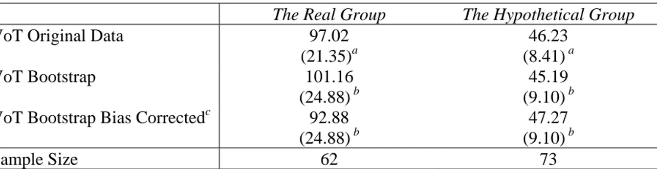
Table 3a presents GMM estimates of the mean value of time (VoT) in the exponential distribution. The VoT estimated on the original sample is seen to be 97 SEK and 46 SEK in the real and hypothetical groups, respectively. The average of the bootstrap estimates is

14

To keep track of any potential trade of tickets in between the experiment and the actual journey, we kept a record of the bus chosen by each subject. No such trades were observed. However, four subjects dropped out. These subjects had all chosen the fast and expensive bus. Their choices are excluded in the analysis.

(17)

somewhat higher in the real group and somewhat lower in the hypothetical group indicating a minor bias of the GMM estimator in the present application. Nevertheless, bootstrap bias corrected estimates are reported at the bottom of the table and seen to be around 93 SEK in the real group and around 47 SEK in the hypothetical group. Note also that the standard deviation of the bootstrap estimates of the VoT is somewhat higher than the corresponding asymptotic standard error of the GMM estimator. This suggests a downward bias in the asymptotic standard errors of the GMM estimator. In sum, all pairs of estimates suggest that the real VoT is approximately twice as large as the hypothetical VoT.

Table 3b reports two t-tests of the difference between the real and the hypothetical VoT. Both of them are applied to the difference between GMM estimates obtained from the original data. The t-test on the first line of the table is, however, based on the asymptotic standard errors whereas the one on the second row is based on the bootstrap standard deviation. Applying a two sided test, both of the tests reject the null hypothesis of no difference at the 10 percent level of significance if we rely on the standard normal approximation. However, and somewhat surprisingly the asymptotically refinement of the t-test suggests that both versions of the t-test reject the null hypothesis at the 5 percent level of significance in a two sided test. The bootstrapped t-distribution exhibits, however, a relatively fat lower tail as compared to the upper tail. This might indicate some problem of the bootstrap to provide asymptotic refinement in the present application. Nevertheless, both approximations of the true finite sample distribution of the t-test in the present application suggest that real and hypothetical mean values of time differ at the 10 percent level of significance.

Table 4a reports GMM estimates of the two parameters of the mixture distribution. The estimates obtained from the original data of the real group indicate that some 50 percent of the sample faces an additional cost of accepting the bid and that the mean value of time among those who do not face such a cost is very low (around 7 SEK) and insignificantly different from zero at conventional levels of significance. The corresponding estimates in the hypothetical group indicate that some 25 percent of the sample face an additional cost of accepting the bid and that the value of time among the 75 percent who do not face such a cost is around 20 SEK. The corresponding bootstrap estimates give similar estimates of the parameters and their standard errors.

(18)

In table 4b, t-tests of the difference between the two estimated parameters of the mixture distribution are reported. Both of the two versions of the t-tests rejects the equality between the fraction (q) of individuals who do not face the additional cost of accepting the bid at the 5 percent level of significance in a two sided test and if the critical values are based on the normal approximations. None of the two versions of the t-test reject the equality between the mean value of time among these individuals at conventional levels of significance.

The lower part of table 4b reports asymptotically refined values of the critical values of the t-test obtained with the bootstrap. The values found for the mean of the exponential distribution among those individuals who do not face the additional cost of accepting the bid are quite different from those obtained with the standard normal approximation. This is probably a consequence of two facts that invalidates the application of the bootstrap in this model. First, the VoT among individuals who do not face the additional cost of accepting the bid is likely to be close to zero which is the boundary constraint of the mean of the exponential distribution Andrews (2001) shows that the bootstrap is inconsistent in this situation. Secondly, Horowitz (2001) notes that whenever the covariance matrix of the estimator is almost singular, the application of the bootstrap is not recommended. This is exactly the case in a number of the bootstrap replications of the mixture model on the present data set. Whenever the estimate was below 1 SEK the covariance matrix was close to singular. In sum, for the mixture distribution applied to the present data, the bootstrap does probably not offer asymptotic refinements of the t-test.

In sum, for the mixture distribution it is better to compare the t-test statistics at the top of the table to critical values of the normal distribution. The results of the test, thus, lend some support the idea of Brownstone and Small (2005) that hypothetical bias in the VoT is due to some kind of scheduling constraint.

4.2 The bus experiment

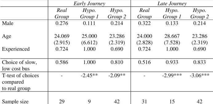
Table 5 presents the results of the bus experiment and descriptive statistics of the participating subjects. The first three columns contain the results for the first journey and the last three columns contain those of the return journey. There are three observable characteristics of the subjects in this experiment: a male dummy variable, age and a dummy variable to indicate

(19)

whether the subject was experienced in going by bus between Borlänge and Falun. Subjects in hypothethetical group 1 are somewhat older and more experienced with bus travels between the two towns than subjects in the real group. But the observable characteristics indicate no significant differences between the real group and hypothetical group 2. In addition, there are no significant differences in terms of observable characteristics between subjects in the real group and the pooled observations of subjects in the two hypothetical groups.

The table also shows that 59 percent of the individuals in the real, all subjects in the first hypothetical and 81 percent in the second hypothetical group chose the slow, low cost bus for the early journey. The difference between the real group and each of the hypothetical groups is significant according to a t-test at the 10 percent level of significance.15 The figures are similar for the late journey. Note also that choice frequencies are quite similar to those found for a bid level of 100 SEK in the survey experiment, both in the real and in the hypothetical groups.

Since Table 5 suggests that individual choices are quite stable between the early and the late journey, only the first choice made of each individual is used when estimating the mean value of time. In addition, since choices in the hypothetical groups seem quite similar in Table 6 and one them is very small, I estimate the mean value of time on a data set that pools observations from the two hypothetical groups. Estimated mean values of time are reported in Table 6. The estimate in the original data of the real group is 115 SEK whereas it is 54 SEK in the hypothetical group. The average bootstrap estimate is 118 and 54 SEK in the real and hypothetical groups, respectively. The bias of the GMM estimator thus appears quite small in this application. So the bootstrap error corrected estimates are 111 SEK and 53 SEK. The asymptotic standard errors appear somewhat below the standard deviations of the bootstrapped estimates. In sum, the real VoT is slightly twice as large as the corresponding hypothetical VoT. The bus experiments, thus, basically replicates the main finding of the survey experiment.

Statistical tests regarding hypothetical bias in the bus experiment are reported in Table 6b. The t-test obtained from the original data and the asymptotic standard errors (first row of the table) and the t-test obtained from the point estimates in the original data and the standard

15

(20)

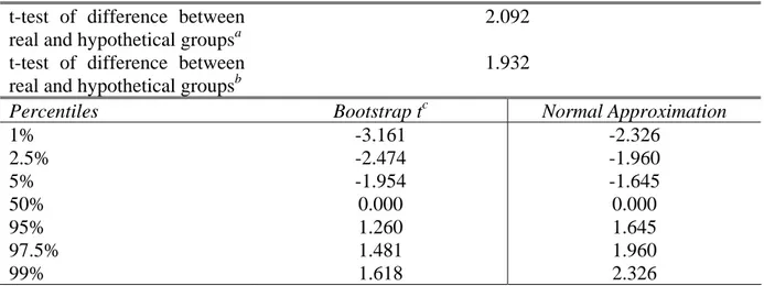
deviations of the bootstrap estimates (second row of the table) are both close to 2. The critical values of the normal approximation thus imply that both versions of the t-test reject the null hypothesis at the 10 percent level in a two sided test. The lower part of the table compares the bootstrapped percentiles of the test to the corresponding percentiles of the normal distribution. As in the survey experiment, the bootstrap approximation of the test statistic’s distribution suggests that the lower part of the distribution is fatter than the upper part. Nevertheless, even with the bootstrapped critical values of a two sided test of the null hypothesis the t-test rejects the null hypothesis at the 10 percent level of significance.

5. CONCLUSIONS

The results of the present paper suggest that there is a bias in estimates of the value of time based on hypothetical choices: real values tend to be higher than values derived from hypothetical choices. This replicates the recent findings of Brownstone and Small (2005) but in a completely different context than they used for their study. Assuming an exponential distribution for the value of time, real choices produced an estimated mean value of time which was more or less equal to some 100 SEK, whereas hypothetical choices lead to an estimate close to 50 SEK. The real mean value of time is thus twice as large as the corresponding hypothetical value. It is interesting to note that this is exactly the same size of the bias as that reported by Brown and Small (2005). The exact magnitude of the bias is, however, likely to depend on the specific assumptions made about the value of time distribution (cf. results reported by Fosgerau, 2006).

The results reported here also lend some support to the conjecture by Brownstone and Small (2005) that the bias results from scheduling constraints that are less pronounced in a hypothetical setting than in a real setting. Estimates presented here suggest that some 50 percent of the subjects in the real group face an unobserved cost of time allocation that makes one alternative better than the other both in terms of money and in terms of time sacrificed. The corresponding figure in the hypothetical group is only 25 percent. Thus, individuals in the hypothetical group might tend to forget scheduling constraints that are not part of the hypothetical choice task whereas this may be unaffordable to individuals making real choices.

(21)

The hypothetical bias also appears to be stable across the experiment and the quasi-experiment this paper. This suggests two things. First, quasi-quasi-experiments with a carefully selected rather than randomized control group may replicate experimental results on hypothetical bias. Secondly, the stability of the bias in the VoT estimates suggests that it is transferable between different contexts. Thus, experiments of the kind reported here may be useful to correct hypothetically derived values of time, as discussed in Harrison (2006) in the context of environmental valuation.

Finally, according to the results obtained with the bootstrap, the small sample bias of the GMM estimator did not appear to be specifically large in the application of this paper. Furthermore, asymptotic refinements of t-tests provided by the bootstrap produced the same conclusions as those obtained from the standard normal approximation, at least at the levels of significance considered here. The bootstrap approximation of the test statistic’s finite sample distribution appeared somewhat asymmetric, however, which might indicate some kind of problem of applying the bootstrap for asymptotic refinements here.

(22)

Acknowledgements

Useful comments were received from the late Peter Bohm, Erika Budh, Kenneth Carling, Lars Hultkrantz, Per Johansson, Chuan-Zhong Li, Lena Nerhagen and Jan-Eric Nilsson. Assistance in the experiments from Gunilla Björklund, Erika Budh, Wilco Burghout, Tobias Heldt, Lars Hultkrantz, Lena Nerhagen and Ola Nääs is gratefully acknowledged. Many thanks to Lars Hultkrantz, Lena Nerhagen and Lars Åberg for their time and effort to give the lectures used in one of the experiments. Comments from seminar participants, in particular from Fredrik Carlsson, at the EIT conference in Borlänge and at Högskolan Dalarna are gratefully acknowledged. Financial support was provided from the Swedish Transport and Communications Research Board. Naturally, I am responsible for any remaining errors.

(23)

REFERENCES

Andrews, D.W.K. (2001), “Testing When a Parameter Is on the Boundary of the Maintained Hypothesis,” Econometrica, 69, pp 683-734.

Altonji and Segal (1996), “Small Sample Bias in GMM Estimation of Covariance Structures,” Journal of Business and Economic Statistics, 14, pp. 353-366.

Bishop, R. and T. Heberlein (1979), “Measuring Values of Extra Market Goods: Are Indirect Measures Biased?,” American Journal of Agriculture Economics, 61, pp. 926-930.

Bohm, Peter (1972), “Estimating Demand for Public Goods: An Experiment,” European Economic Review, 3, pp. 111-130.

Boxall, Peter C., Wiktor L. Adamovicz, Joffre Swait, Michael Williams and Jordan Louviere (1996), “A comparison of stated preference methods for environmental valuation,” Ecological Economics, 18, pp. 243-253.

Brookshire, David S. and Don L. Coursey (1987), “Measuring the Value of a Public Good: An Empirical Comparison of Elicitation Procedures,” American Economic Review, Vol. 77, No. 4, pp.554-566.

Brownstone, David and Kenneth A. Small (2005), “Valuing time and reliability: assessing the evidence from road pricing demonstrations,” Transportation Research Part A, 39

Carlsson, Fredrik and Peter Martinsson (2001), “Do Hypothetical and Actual Marginal Willingness to Pay Differ in Choice Experiments?,” Journal of Environmental Economics and Management 41, pp. 179-192.

Cameron, A. Colin and Pravin K. Trivedi (2005), Microeconometrics: Methods and Applications, Cambridge University Press: New York.

Cummings, Ronald G., Steven Elliott, Glenn W. Harrison, and James Murphy, (1997), “Are Hypothetical Referenda Incentive Compatible?,” Journal of Political Economy, 105(3), pp.609-621.

Cummings, Ronald G., Glenn W. Harrison, and E. Elisabeth Rutström, (1995), “Homegrown Values and Hypothetical Surveys: Is the Dichotomous Choice Approach Incentive-Compatible?”,” American Economic Review, 85(1), pp.260-266.

Cummings, Ronald G. and Laura Taylor (1999), “Unbiased Value Estimates for Environmental Goods: A Cheap Talk Design for the Contingent Valuation Method,” American Economic Review, Vol. 89, No. 3, pp. 649-665.

DeSerpa, A. (1971), “A Theory of the Allocation of Time”, The Economic Journal 81, 828-846.

Fosgerau, Mogens (2006), “Investigating the distribution of the value of travel time savings,” Transportation Research Part B, 40, pp. 688-707.

(24)

Frykblom, Peter (1997), “Hypothetical Question Modes and Real Willingess to Pay,” Journal of Environmental Economics and Management 34, pp. 274-287.

Hall, Peter and Joel L. Horowitz (1996), “Bootstrap Critical Values for Tests Based on Generalized-Method-of-Moments Estimators,” Econometrica, 64(4), pp. 891-916.

Hansen, L.P. (1982), “Large Sample Properties of Generalized Method of Moments Estimators,” Econometrica, pp. 1029-1054.

Harrison, Glenn W. (2006), “Experimental Evidence of Alternative Environmental Valuation Methods,” Environmental and Resource Economics 34, pp 125-162.

Heckman, James J. and Hotz (1989), “Choosing Among Alternative Non-Experimental Methods for Evaluating the Impact of Social Programs,” Journal of the American Statistical Association, 84, pp. 862-880.

Hensher, D. A. and A.M. Brewer (2001), Transport an economics and management perspective, Oxford: Oxford University Press.

Horowitz, Joel L. (2001), “The Bootstrap,” in Handbook of Econometrics, J.J. Heckman and E. Leamer (eds), Volume 5, pp 3159-3228, Amsterdam, North-Holland.

List, John A. and Jason F. Shogren (1998), “Calibration of the difference between actual and hypothetical valuations in a field experiment,” Journal of Economic Behavior & Organization, Vol. 37, pp. 193-205.

Louviere, Jordan J., David A. Hensher and Joffre D. Swait (2000), Stated Choice Methods – Analysis and Application, Cambridge University Press.

Neill, Helen R., Ronald G. Cummings, Philip T. Ganderton, Glenn W. Harrison and Thomas McGuckin, (1994), “Hypothetical Surveys and Real Economic Commitments”, Land Economics, 70(2), pp. 145-154.

Smith, V. Kerry and Carol Mansfield (1998), “Buying Time: Real and Hypothetical Offers,” Journal of Environmental Economics and Management, 36, pp. 209-224.

Truong, T. P. and D. A. Hensher (1985), “Meaurement of Travel Time Values and Opportunity Cost from a Discrete-Choice Model”, The Economic Journal 95, 438-451.

(25)

Table 1. The Survey Experiment: Descriptive Statistics, Means and Standard Deviation

The Real Group The Hypothetical Group

Male 0.21 0.32 Age 28.6 (7.60) 27.0 (6.58) Sample Size 62 73

Table 2. The Survey Experiment: Choices

The Real Group The Hypothetical Group Test for difference Accept Bid = 5,

(Number of subjects receiving the bid)

0.45 (22) 0.48 (21) t-test (df 41) = -0.14 Accept Bid = 15,

0.50 (22) 0.74 (23) t-test (df 43) = -1.67 Accept Bid = 25,

0.50 (18) 0.76 (29) t-test (df 45) = -1.85* Total (Number of subjects) 0.48 (62) 0.67 (73) Chi-Square (df 1) = 4.19**

Notes: * Rejects null hypothesis at 10 percent level of significance. ** Rejects null hypothesis at 5 percent level of significance.

Table 3a. The Survey Experiment: Mean Value of Time (Exponential Distribution)

VoT Original Data 97.02

(21.35)a 46.23 (8.41) a VoT Bootstrap 101.16 (24.88) b 45.19 (9.10) b VoT Bootstrap Bias Correctedc 92.88

(24.88) b

47.27 (9.10) b

Sample Size 62 73

Notes: (a) Asymptotic standard errors within parenthesis for the two-step GMM estimator. (b) Standard deviations for the bootstrap applied to the two step GMM estimator with recentering of moment conditions. (c) The difference between 2 times the ‘VoT Original Data’ and ‘VoT Bootstrap’.

(26)

Table 3b. Bootstrap Inference for Hypothetical Bias in Parameter of the Exponential Distribution

t-test of difference between real and hypothetical groupsa

2.213

t-test of difference between real and hypothetical groupsb

1.917

Percentiles Bootstrap tc Normal Approximation

1% -2.790 -2.326 2.5% -2.331 -1.960 5% -1.839 -1.645 50% 0.040 0.000 95% 1.552 1.645 97.5% 1.804 1.960 99% 2.104 2.326

Notes: (a) Applied to the difference between the estimated mean values of time in the original data and the corresponding asymptotic standard errors. (b) Applied to the difference between the estimated mean values of time in the original data and the corresponding asymptotic standard errors. (c) Based on the bootstrap applied to the two-step GMM estimator with recentered moment conditions and with the t-statistic centered on the difference between the estimated mean values of time in the original data.

Table 4a. The Survey Experiment: Mean Value of Time (Mixture Distribution)

Parameter q Mean of Exponential q Mean of Exponential Original Data 0.490 (0.080) 7.610 (10.645) 0.760 (0.075) 19.730 (8.972) Bootstrap 0.512 (0.097) 9.764 (12.095) 0.779 (0.088) 21.060 (10.536) Bootstrap Bias Correctedc 0.468

(0.097) 5.456 (12.095) 0.741 (0.088) 18.400 (10.536) Sample Size 62 73

Notes: (a) Asymptotic standard errors within parenthesis for the two-step GMM estimator. (b) Standard deviations for the bootstrap applied to the two step GMM estimator with recentering of moment conditions. (c) The difference between 2 times the ‘VoT Original Data’ and ‘VoT Bootstrap’.

(27)

Table 4b Bootstrap Inference for Hypothetical Bias in Parameters of the Mixture Distribution

Parameter q Mean of Exponential

-2.466 -0.871

-2.064 -0.756 Percentiles Bootstrap tb q Mean of Exponential 1% -1.960 -0.867 2.5% -1.700 -0.682 5% -1.404 -0.437 50% 0.000 0.000 95% 1.562 1.270 97.5% 1.843 1.429 99% 2.335 1.559

Notes: (a) Applied to the difference between the estimated mean values of time in the original data and the corresponding asymptotic standard errors. (b) Applied to the difference between the estimated mean values of time in the original data and the bootstrap standard errors. (c) Based on the bootstrap applied to the two-step GMM estimator with recentered moment conditions and with the t-statistic centered on the difference between the estimated mean values of time in the original data.

Table 5. The Bus Experiment: Choices and Descriptive Statistics, Means and Standard Deviations

Early Journey Late Journey

Real Group Hypo. Group 1 Hypo. Group 2 Real Group Hypo. Group 1 Hypo. Group 2 Male 0.276 0.111 0.214 0.322 0.133 0.214 Age 24.069 (2.915) 25.000 (6.612) 23.286 (2.319) 24.000 (2.828) 28.667 (7.528) 23.286 (2.319) Experienced 0.724 1.000 0.690 0.724 1.000 0.690 Choice of slow, low cost bus

0.586 1.000 0.810 0.516 0.933 0.833 T-test of choices compared to real group - -2.45** -2.09** - -2.99*** -3.06*** Sample size 29 9 42 31 15 42

Notes: Standard deviations in parentheses. All subjects participating in the experiment for the late, but not for the early journey, have missing values for the experience variable.

(28)

Table 6. The Bus Experiment: Mean Value of Time (Exponential Distribution)

VoT Original Data 115.08 (27.99)a 53.68 (8.83)a VoT Bootstrap 118.80 (30.49) b 53.88 (8.97) b VoT Bootstrap Bias Correctedc 111.36

(30.49) b

53.48 (8.97) b

Sample Size 31 58

Notes: Estimates are based on first choices only. (a) Asymptotic standard errors within parenthesis for the two-step GMM estimator. (b) Standard deviations for the bootstrap applied to the two two-step GMM estimator with recentering of moment conditions. (c) The difference between 2 times the ‘VoT Original Data’ and ‘VoT Bootstrap’.

Table 6b. Bootstrap Inference for Hypothetical Bias in Parameter of the Exponential Distribution - the Bus Experiment

2.092

1.932

Percentiles Bootstrap tc Normal Approximation

1% -3.161 -2.326 2.5% -2.474 -1.960 5% -1.954 -1.645 50% 0.000 0.000 95% 1.260 1.645 97.5% 1.481 1.960 99% 1.618 2.326

Notes: (a) Applied to the difference between the estimated mean values of time in the original data and the corresponding asymptotic standard errors. (b) Applied to the difference between the estimated mean values of time in the original data and the corresponding bootstrap standard errors. (c) Based on the bootstrap applied to the two-step GMM estimator with recentered moment conditions and with the t-statistic centered on the difference between the estimated mean values of time in the original data.

(29)

Appendix A. The bootstrap GMM procedure

The parameters of F

( )

b,μ in the survey experiment are estimated with a two-step GMM estimator. In the first step equal weights are applied to the three moment conditions. That is, the step 1 estimate of solves μ

mm' μ min , (F4) where m

(

5

(

20,μ

)

, 15

(

60,μ

)

, 25

(

100,μ

)

1 1 100 1 1 60 1 1 20 y F n y F n y F n i n i n i n − − − = −

∑

−

∑

−

∑

The optimal weight matrix for the second step is adapted for the fact that a split sample approach is used; i.e. the optimal weight matrix is a diagonal matrix, so the estimated optimal weight matrix for the second step is

1 1 , 1 , , 1 , 1 1 ˆ − = − − ⎥ ⎦ ⎤ ⎢ ⎣ ⎡ =

∑

nb i b i b i b m m n diag V

where mˆ_i_,₁_,_b = y_i −F

(

b,μˆ₁

)

and μˆ₁ is the solution to F4. The second step estimate of solves μ m' V m μ 1 ˆ min − , (F5)

The asymptotic standard errors of this estimator of is obtained from the following covariance matrix μ

( )

(

₁

)

1 ' ~ ˆ = gV−g − μ V

where g=

(

n₂₀1/2f

(

20,μˆ₂

)

,n1₆₀/2f

(

60,μˆ₂

)

,n₁₀₀1/2f

(

100,μˆ₂

)

, is the solution to F5, is the density function corresponding to

2

ˆ

μ f

(

b, μˆ2

)

(

b, μˆ2

)

F and is defined in the same way as with used instead of the first-step estimator .

1 ~− V _V_ˆ−1 2 ˆ μ μˆ1

(30)

All standard errors and tests regarding this estimator of are computed from 999 parametric bootstrap samples taken from empirical binomial distributions implied by observed choices and sample sizes (see, for example, Cameron and Trivedi, p. 360). The bootstrap estimates of are based on the recentered moment conditions M2 rather than M1, where is the solution to F5 in the original data. Beside the fact that M2 is used instead of M1, each bootstrap estimate of is obtained in the same way as .

μ

μ μˆ₂

The asymptotic refinement of the t-test statistics distribution is based on the following statistic applied to a specific element (μ) of μ ,

(

) (

)

(

)

(

₂ ₂

)

1/2 * b b h o r o h b r b b sh sr t + − − − = μ μ μ μ

where b = 1, 2, …, B refers to a specific bootstrap replication, ( ) is the estimate obtained in bootstrap sample b of the real (hypothetical ) group, ( ) is the estimate obtained in the original data of the real (hypothetical) group, ( ) is the asymptotic standard error pertaining to ( ).

r b μ h b μ r o μ h o μ b sr shb r b μ h b μ

(31)

Appendix B: Instructions for the survey experiment

After subjects had completed the first questionnaire on their traffic behavior, they were given the following instructions. Bold text was specific to the real group and it was exchanged for text in italics in the hypothetical group.

“The group of researchers that has constructed the questionnaire, has also constructed another questionnaire which is similar to the one that you just completed. That questionnaire will also take 15 minutes to complete. We offer you/Suppose that you would be offered to fill in the second questionnaire here and now. After/Suppose also that after you have/would have completed that questionnaire we will/we would pay you X16 SEK for your trouble.

Question: Do you/ Would you agree to fill in that questionnaire also?

Observe that those who answer no to the question will be free to leave the room as soon as we see that each one has indicated their answer. Those that answer yes to the question will fill in the second questionnaire. After fifteen minutes they will get their money and will subsequently be free to leave the room./Observe that you will be free to leave the room independent of how you answer, as soon as we see that each one of you has indicated their answer.

Indicate your answer here: Yes No

Thank you for participating!

Observe that all kinds of communication are still forbidden!”

16

(32)

Appendix C: Instructions for the bus experiment

The following instructions were given to the real group.

“You will now participate in an experiment on decision making. You are not allowed to communicate with each other during the experiment. If you have any questions, please raise your hand so that you can ask me quietly. If I think that the question is relevant for the entire group, I will repeat the question and answer it for the whole group.

There will be two buses from Borlänge to Falun to take you to the lectures. One of these will take a direct route and it will leave at 8.30 a.m. from the parking lot outside the university building in Borlänge. It will arrive around 8.55 a.m. right outside the university building in Falun. This bus will cost you 50 SEK. The amount will be subtracted from the 150 SEK that you get for participating in this experiment.

The other bus will pass Aspeboda to pick up some people there. This bus will leave at 8.15 a.m. from the parking lot outside the university building in Borlänge. It will also arrive around 8.55 a.m. right outside the university building in Falun. This bus will cost you 25 SEK. The amount will be subtracted from the 150 SEK that you get for participating in this experiment.

Indicate your choice of bus on the questionnaire that I now will distribute. When everybody has made their choice, I will collect the questionnaires and give each one of you a ticket for the bus that you have chosen. You will have to show the ticket on the bus. All payments for participating in this experiment will be made on the bus. Thus, if you do not use the chosen bus, you will not earn any money for participating in this experiment.”

The following instructions were given to the first hypothetical group.

(33)

A bus between the university buildings in Borlänge and Falun can either take a direct route or an indirect route. The bus does not take the shortest route in the latter case but stops at different places along the route to pick up people. This implies that if you were to travel between the university buildings in Borlänge and Falun, your travel time and travel cost can be affected.

Suppose that you would make a journey by bus tomorrow morning between the university’s buildings in Borlänge and Falun. We will now present you with two alternatives for this journey. Indicate your preferred alternative. Suppose also that the buses depart at different points in time but arrive at the same time.

Indicate your choice of bus on the questionnaire that we now will distribute.”

The following instructions were given to the second hypothetical group.

Suppose, first of all, that you would attend a series of lectures on the theme writing for academic purposes in the university’s building in Falun that begins at 9.00 a.m. and that you would need to travel between Borlänge and Falun. Suppose, secondly, that there would be two buses going between the university buildings in Borlänge and Falun.

Suppose, thirdly, that one of these buses takes a direct route leaving at 8.30 from the parking lot outside the university building in Borlänge and it will arrive at around 8.55 a.m. right outside the university building in Falun. This bus would cost you 50 SEK. Suppose also that this amount would be subtracted from the 150 SEK that you get for participating in this experiment.

(34)

Suppose, fourthly, that the other bus passes Aspeboda to pick up some people there. This bus will leave at 8.15 a.m. from the parking lot outside the university building in Borlänge. It will also arrive around 8.55 a.m. right outside the university building in Falun. This bus would cost you 25 SEK. Suppose also that this amount would be subtracted from the 150 SEK that you get for participating in this experiment.

Indicate your choice of bus on the questionnaire that I now will distribute. When everybody has made their choice, I will collect the questionnaires.”

Subjects in all three groups received the following questionnaire to indicate their choice.

----

Indicate your choice with a cross in the square under your preferred alternative.