ON THE ANALYTICS OF THE DYNAMIC LAFFER CURVE
* byJonas Agell
aand Mats Persson
bAbstract
In this paper, we analyze government budget balance within a simple model of
endogenous growth. For the AK model, simple analytical conditions for a tax cut to be self-financing can be derived. The critical variable is not the tax rate per se, but the ”transfer-adjusted tax rate”. We discuss some conceptual issues in dynamic revenue analysis, and we explain why previous studies have arrived at seemingly contradictory results. Finally, we perform an empirical study of the transfer-adjusted tax rates of the OECD countries to see which country has the highest potential for fiscal
improvements; it turns out that only a few countries have any potential for such ”dynamic scoring”.
Keywords: Laffer effects, intertemporal models, dynamic scoring, growth models JEL Classification: E62; O41
*
We have benefited from presenting the paper at Uppsala University; the Institute for International Economic Studies, Stockholm University; and the Stockholm School of Economics.
a
Department of Economics, Uppsala University, Box 513, SE-751 20 Uppsala, Sweden. E-mail: jonas.agell@nek.uu.se.
b
Institute for International Economic Studies, Stockholm University, SE-106 91 Stockholm, Sweden. E-mail: mats.persson@iies.su.se.
1. Introduction
One of the most controversial issues in tax policy analysis is whether a tax cut will boost economic activity to such an extent that the government’s budget actually improves. Traditionally, this has been discussed in the context of static models, and the question has been whether the labor supply elasticity is large enough for self-financing tax cuts to be possible.1 In contrast, much less is known about possible Laffer effects in a dynamic context. In view of the massive interest during the last decade in growth theory, and in studies of the optimality of intertemporal tax policy, this is surprising. To a political decision-maker, possible Laffer-curve effects may seem much more tangible than the subtle welfare effects usually analyzed in the literature on taxation and economic growth.
In the present paper, we will derive results that shed light on the nature of dynamic Laffer effects. Since there are many varieties of endogenous growth models, we will confine our analysis to the simplest one, namely the AK model.2 For this work horse model, quite a few analytical results can actually be obtained. It also provides the kind of clean environment which is useful if one wants to explore some
fundamental conceptual issues. By means of illustrative calculations for the OECD, we will also try to highlight the scope for dynamic Laffer effects in the real world.
To our knowledge, there are only two previous papers that deal with the issue of whether a tax cut will finance itself in endogenous growth models. Based on
numerical simulations of an AK model, Ireland (1994) concludes that a ceteris paribus reduction in the marginal tax rate “...can be the key to both vigorous rates of real growth and long-run government budget balance in the U.S. economy today” (p. 570). However, using a similar model, Bruce and Turnovsky (1999) conclude that dynamic
1
See e.g. Fullerton (1982) and Malcolmson (1986). 2
Laffer effects will not occur in practice – according to them a ceteris paribus tax cut can only improve the long-run fiscal balance if the intertemporal elasticity of
substitution is (much) above unity, a possibility which they rule out on empirical grounds.
As we show below, an important reason for these conflicting results is that there are alternative ways of defining a ceteris paribus tax cut in a dynamic model. According to our own preferred definition, a government may indeed cut the income tax, and improve the long-run fiscal position, even though the intertemporal elasticity of substitution is less than unity. Yet, our stylized numerical examples suggest that lower taxes on capital is no free lunch for the U.S. economy; an isolated tax cut boosts growth, but this occurs at a cost in the form of a deteriorating long-run budgetary position. When we re-calibrate our model to reflect a stylized European welfare state, with a higher tax rate, and generous transfer schemes, matters look different. We can not rule out the possibility that some countries are in the vicinity of – or beyond – the peak of the dynamic Laffer curve.
2. The model
2.1 Households
Consider a one-sector economy, where production is linear in the private stock of capital:
AK K
f
Y = ( )= . (1)
In the following, we may think of K as including human capital as well as physical capital. Since it is immaterial to our problem, we assume a constant population and no
physical depreciation of capital. Also, to save on notation we omit time indices. In a competitive market, the interest rate is equal to the marginal product of capital:
A K f
r = '( )= . (2)
Since A is an exogenous technological constant, the market interest rate is a constant which is independent of tax policy.
At each instant our infinitely-lived representative consumer derives utility from consuming an ordinary consumption good, C, and a public good G, provided by the government. In the instantaneous felicity function C and G show up as additively separable variables, which means that the intertemporal utility function is of the form3
[
]
∫
∞ − + = 0 ) ( ) (C v G e dt u U θt . (3)Like in virtually all models of endogenous growth we will assume that u(C) is of the iso-elastic variety, implying that the intertemporal rate of substitution
) ( ) (C Cu C u′ ′′ − ≡
σ reduces to a positive constant.
The representative consumer earns the market rate of interest r on her net wealth, W, which consists of the sum of physical capital, K, and debt issued by the government, B. Asset income is taxed at the proportional tax rate τ (assumed to be constant over time). We assume that the government provides the consumer with a (possibly time-dependent) lump-sum transfer T. The flow budget constraint of the consumer is therefore C T W r W& = (1−τ) + − , (4)
where W ≡K+B, and where initial wealth W is a given constant. Maximizing (3) 0
subject to (4) gives us the Euler equation:
3
We have also worked out the analytics for a utility function which is multiplicatively separable in C and G. It turns out that our main results go through also in this case; see Appendix for further details.
[
τ θ]
γ σ − − ≡ = A(1 ) C C& , (5)where we have made use of (2). Since the real rate of interest is a constant, consumption grows at a constant exponential rate. To ensure that the steady-state growth rate γ is positive in the absence of taxes, we assume
θ
>
A . (6a)
We also need the transversality condition
0 lim − = ∞ → t t t t W e θ λ ,
where λ is the current-value costate variable of the optimization problem. Working t out the optimal path of W by applying (5), it can easily be shown that the t
transversality condition is satisfied if and only if (σ −1)A(1−τ)−σθ <0. If this inequality holds in the absence of taxes (i.e. for τ =0), it also holds for all τ ∈[0,1]. Thus, we will assume from now on that the parameters always satisfy
0 )
1
(σ − A−σθ < . (6b)
This assumption thus guarantees that the transversality condition will always be satisfied. Together with (6a) it will prove useful in signing some of the comparative statics results derived below.
Integrating (4) and (5), it is a standard exercise to derive
t t C e C = 0 γ , (7a) where + ⋅ =
∫
∞ − − 0 ) 1 ( 0 0 mpc W Te dt C A τ t . (7b)The marginal propensity to consume out of total private wealth (inclusive of transfers), mpc, is defined as
σθ σ τ γ τ − ≡ − − + − ≡ A(1 ) A(1 )(1 ) mpc . (7c)
Here, it is useful to keep in mind that a tax cut affects C via two channels. First, a 0
lower τ increases the after-tax discount rate used by consumers to compute the present value of transfers (the second term within brackets in (7b)). This creates a negative wealth effect, which lowers C . Second, a lower τ affects mpc. The sign of this effect 0 depends on the magnitude of the intertemporal elasticity of substitution, σ . From (7c), it follows readily that
) 1 ( σ τ =− − ∂ ∂ A mpc , (7d)
i.e., a lower τ reduces the marginal propensity to consume out of current total wealth if and only if σ >1.
2.2 The intertemporal resource constraint
The government’s current revenue consists of the income from distortionary taxes,
AW
τ . The government’s current spending consists of lump-sum transfers, purchases of private goods that are immediately transformed into public ones (think of the fire department), and interest payments on the stock of government debt. We can thus write the government’s flow budget constraint as
AW AB T G
B& = + + −τ , (8)
where initial debt B is a given constant. The government respects the customary 0
solvency constraint, which implies that Bte−A(1−τ)t →0 as t→∞. The intertemporal budget constraint of the government then becomes:
∫
∫
∞ − ∞ − = + + 0 0 0 (G T)e dt B dt We A At At τ . (9)Equation (9), or slight variations of it, is the starting point for the dynamic revenue investigations of e.g. Ireland (1994) and Bruce and Turnovsky (1999).
An equivalent, but in our view more illuminating, approach is as follows. Combining the consumer’s flow budget constraint (4), and the government’s flow budget constraint (8), we obtain the economy’s aggregate resource constraint
G C K
AK = & + + . (10)
Integrating (10), invoking (6b), which implies that lim − =0
∞ → t A t t K e , we obtain the
intertemporal version of the aggregate resource constraint:
G A C K + − = γ 0 0 , (11) where
∫
∞ − ≡ 0 dt GeG At . The initial stock of capital, K , must equal the sum of the 0
present values of private and public consumption.4 Since initial consumption C and 0
the consumption growth rate γ depend on the government’s tax and transfer
programs, (11) is more informative than a mere accounting identity. In fact, (11) can be used as a highly intuitive tool for students of dynamic fiscal policy. For any given tax rate τ , and any given transfer program (Tt)∞0 , one can compute the present value of private consumption, using (7a)-(7c). Using (11) it is then straightforward to compute the residual, G , that is left over for public consumption. It is by studying
how changes in the tax rate τ affects the magnitude of this residual that we can
2.3 Two definitions
In a static setting there appears to be no ambiguity concerning the definition of a Laffer effect – if a ceteris paribus tax cut produces a contemporaneous revenue gain there is a Laffer effect. However, in a dynamic setting, where a tax cut affects the growth rate, the precise meaning of ceteris paribus is open to debate. Consider an initial equilibrium of balanced growth, where the government lets both public consumption and transfers grow at the same rate as output. There are now two main ways of exploring the dynamic revenue effects from a lower tax rate. The first is to study the revenue implications under the assumption that the government sticks to its original consumption and transfer programs, in spite of the fact that a tax cut boosts the growth rate of output. As a consequence, the share of aggregate resources which is channeled through the government will start to decrease, once the tax cut is
implemented. The second is to assume that the government is committed to maintain constant ratios of spending to output also after the tax cut. As a consequence, a tax cut must now be accompanied by an expansionary spending policy, so that the growth rate of government spending keeps up with the increase in the growth rate of output.
As we will show below, these polar ways of defining the ceteris paribus goes a long ways towards explaining why previous studies of dynamic Laffer effects have reached conflicting conclusions. Ireland (1994) analyzes under what conditions a tax cut allows the government to raise a stream of tax revenues with the same present value as before, and he assumes that the government continues to carry out its original transfer program, even though output grows at a higher rate. Bruce and Turnovsky (1999) analyze how the long-run fiscal balance is affected by a tax cut, accompanied 4
Here, and in the following, note that the present values that appear in the aggregate resource constraint are computed using the discount rate A, which is independent of the tax rate. The present value of transfers that appear in the consumption function (7b) is computed using the after-tax discount rate A(1−τ).
by those changes in the government’s spending policies which are required to maintain a constant public sector share of the economy.
More formally, we may define the two competing definitions of a dynamic Laffer effect as follows, the first one being
DEFINITION 1. Assume that (11) applies for some initial tax rate τ , and for some
initial sequences of public consumption and transfers, (Gt)∞0 and (Tt)∞0. A dynamic Laffer effect is said to occur if there is some lower tax rate
τ′, which allows the government to increase at least one of the elements in either (Gt)∞0 or (Tt)∞0 , while keeping the other elements the same.
The definition is obviously quite general, and not tied to the specifics of the AK model. Conceptually, it is kindred in spirit to the ceteris paribus approach of the literature on static revenue gains. It is also equivalent to the approach of Ireland (1994), in that it does not assume that the government automatically implements whatever fiscal policies that are needed to maintain the public sector’s relative share of the economy. Our second definition presupposes that the government sets the growth rate of public spending equal to the current growth rate GDP:
DEFINITION 2. Assume that (11) applies for some initial tax rate τ , and for some initial sequences of public consumption and transfers, (Gt)∞0 and (Tt)∞0. These sequences are such that G and T grow at the same rate as output, so that Gt Yt and Tt Yt are constant over time. A dynamic Laffer effect is said to occur if there is some lower tax rate τ′ which allows a higher
constant ratio of either public consumption to output, or of transfers to output.
3. Dynamic Laffer effects according to DEFINITION 1
Let us see what happens to government consumption if we change the tax rate. Rewriting the aggregate resource constraint (11), we obtain:
γ − − = A C K G 0 0 . (12)
According to DEFINITION 1 there is a dynamic Laffer effect if a lower income tax rate
allows the government to increase public consumption, today or sometimes in the future. This is equivalent to asking under what circumstances a lower tax rate allows the government to increase G , i.e. we ask under what circumstances the derivative
τ d G
d is negative. From (12) it is easy to see that
0 < τ d G d if and only if
(
)
0 0 0 > ∂ ∂ + ∂ ∂ − τ γ τ γ C C A , (13)where it follows from (5) and (7b) that
τ τ τ τ τ ∂ ∂ ⋅ + + ⋅ ∂ ∂ = ∂ ∂
∫
∫
∞ − − ∞ − − 0 ) 1 ( 0 ) 1 ( 0 0 dt Te mpc dt Te W mpc C t A t A (14a) A σ τ γ =− ∂ ∂ . (14b)According to (12) a lower tax rate must be accompanied by a lower present value of private consumption, C0 (A−γ), if G is to increase. But as a tax cut leads to an unambiguous increase in γ , which in itself tends to increase the present value of private consumption, a dynamic Laffer effect will only come forth if there is a
sufficiently large drop in current consumption, C . In terms of (13), this implies that 0
the first term, involving the derivative ∂C0 ∂τ , must take on a sufficiently large
positive value to dominate the second term, which is always negative.
We can now derive a startling result. Assume that there are no transfers in the economy, which implies that all tax revenue is used for government consumption. It must then be the case that C0 =mpc⋅W0, and that (14a) reduces to 0 0
W mpc C ⋅ ∂ ∂ = ∂ ∂ τ τ .
Equation (12) then implies
) ) 1 ( ( ) ( sgn sgn , 0 σ τ θ θ σ τ − − − − − = ∀ = A A A A d G d t T . (15)
But because of the transversality condition in (6b), both the numerator and the denominator on the right hand side of (15) must be positive. We have thus proved:
PROPOSITION 1: If there are no transfers, there can never be a dynamic Laffer effect in
the sense of DEFINITION 1.
In an AK model without transfers, a higher tax rate will always increase the scope for public consumption. Although it is true that a tax cut stimulates growth in the tax base, this stimulus can never be large enough to compensate for the revenue loss from a lower tax rate on the existing capital stock. A government that has as its sole purpose to maximize the level of public consumption will find it profitable to raise the tax rate, in spite of the adverse effect on economic growth. A revenue-maximizing government will in fact set the income tax rate equal to 100 percent. At this confiscatory rate, G reaches its maximum, but the growth rate is minimized;
COROLLARY 1: In an economy without transfers, the revenue-maximizing income tax
rate is 100 percent. At this rate, growth is negative, and equal to −σθ.
To understand the intuition, consider the last term on the right-hand side of equation (14a). Clearly, the existence of a predetermined transfer program increases the likelihood that a tax cut produces the kind of drop in initial consumption which is required for a dynamic Laffer effect to come forth. Since the private sector’s discount rate is the after-tax interest rate A(1−τ), a lower value of τ means more heavy discounting5, that is, a fall in the present value of the transfer stream (Tt)∞0 . In an economy without transfers, this negative walth effect is absent. Provided that σ >1, a tax cut will still be accompanied by a reduction in C (this follows from (7d)), but this 0
reduction is too modest to deliver a reduction in the present value of consumption. Let us then return to the general case, when there are both transfers and public consumption. For this end, it is helpful to consider the case when transfers grow at some predetermined exponential rate γ , so that
t
e T
T = 0 γ , (16)
which implies that the present value of transfers in (14a) becomes T0/
(
A(1−τ)−γ)
. For the case of an initial balanced growth equilibrium – i.e., γ equals theconsumption growth rate in the initial equilibrium, before the tax cut – it is straightforward to express (13) as6
PROPOSITION 2: 0 < τ d G d if and only if 0 0 ) ) 1 ( ( ) ( C T A A A A < − − − − − θ τ σ θ σ . (17)
PROPOSITION 2 brings out the key role of transfers in making a dynamic Laffer effect possible.7 In an economy where a relatively large share of private consumption is financed via transfers, a tax cut will create a relatively large negative wealth effect, which increases the likelihood that C drops by the required amount. 0
An interesting special case of (17) is when there is no initial government consumption, i. e. we set G =0 for some given transfer stream (Tt)∞0 . This is exactly the problem studied by means of numerical simulations by Ireland (1994), who offers his analysis as theoretical evidence that tax cuts will, for reasonable parameter configurations, improve both growth and the long-run budget balance of the government. From (17) we can see that there is in fact a closed-form solution to Ireland’s problem. Setting G =0 in (12), and substituting the resulting expression for
0 C into (17), we have COROLLARY 2: 0 0 0 ) ( 0 K T A A if only and if d G d G < − − < = θ σ τ , (18) 5
Note that the equivalent of PROPOSITION 1 might not hold for growth models where the pre-tax interest rate is endogenous.
6
The case of γ >γ is not interesting since it implies that transfers will sooner or later exceed GDP. For the case of γ <γ , which means that transfers will approach zero as a fraction of GDP, one can derive an expression corresponding to (17).
which is considerably simpler than (17) since it contains only exogenous variables. Equation (18) sheds light on why Ireland (1994) had no difficulty finding numerical parameter values for which tax cuts boosted the long-run public budget. Since he assumes that all distortionary tax revenue is used to finance predetermined transfers, his setup is maximally favorable to the existence of a dynamic Laffer effect. Indeed, it is not at all difficult to come up with plausible parameter configurations which will guarantee that (18) holds true.
4. Dynamic Laffer effects according to DEFINITION 2
Let us now turn to the possibility of a dynamic Laffer effect in the sense of DEFINITION 2. As a consequence, we no longer assume that G and T follow some
predetermined growth paths; we rather assume that the government always sets the growth rate of both public consumption and transfers equal to the growth rate of GDP:
t e G G = 0 γ (19) t e T T = 0 γ . (20)
After substituting these equations into (12), and differentiating implicitly, we can now explore whether a lower τ allows the government to maintain a higher ratio of either
7
Since we have argued above that a dynamic Laffer effect can be equivalently defined as a possible increase in G, keeping transfers constant, and as a possible increase in transfers, keeping G constant, one may ask whether the condition that dT0 dτ <0 is the same as the condition that dG dτ <0. The answer is yes. To see this, differentiate (12) with respect to τ and T0, treating G as fixed. After some
0 0 / Y
G or T0/ Y0. Since AK is exogenously given, all information about these ratios 0
is in the derivatives dG /0 dτ and dT /0 dτ.
8 We obtain 0 0 < τ d dG if and only if A
[
K0 +B0(1−σ)]
<0. (21) The inequality condition (21) gives us necessary and sufficient conditions for a dynamic Laffer effect to obtain, in the sense of DEFINITION 2.Can this condition ever be satisfied? Bruce and Turnovsky (1999) seem to think so.9 They state (in their Proposition 1, on p. 172) that a necessary condition for Laffer curve effects to obtain is that σ >1, a condition that conforms well to our condition (21). They then reject this condition on the empirical ground that
econometric studies (discussed below) indicate that σ is in fact below unity. We will now show analytically that as long as the consumer’s solvency constraint (6b) is satisfied, there can not be any Laffer effects regardless of the value of σ . We will thus dismiss Laffer effects according to DEFINITION 2 in the AK model on theoretical grounds.
Assume that a dynamic Laffer effect is possible. By (21) it must then hold that 0 ) 1 ( 0 0 +B −σ < K . (22)
Since G, T, C and W always grow at the same rate γ, (9) and (11) can be written as ) /( ) ( ) /( 0 0 0 0 γ γ τAW A− =B + G +T A− and K0 =C0/(A−γ)+G0 /(A−γ), respectively. Combining these expressions with (22), we obtain
) 1 )( ( 0 0 0 0 0 +C < τAW −G −T σ − G . (23) 8
By the same reasoning as in the previous footnote one can show that dG /0 dτ has the same sign as
τ d
dT /0 . Thus, it is again sufficient to concentrate on just one of the two derivates. 9
Bruce and Turnovsky (1999) use a more complicated model, which also includes productive public investments and a utility function which is multiplicative in C and G (like the one analyzed in our Appendix). Basically, however, their model is an AK model, just like ours.
The expression for C0 is obtained from (7b) and (7c). Substituting this into (23), and
rearranging terms, yields (A−γ)W0 <σ(τAW0 −G0 −T0). Recalling the definition of
γ from (5) we finally have that the inequality
) (
)) (
(A−σ A−θ W0 <−σ G0 +T0 (24)
must be satisfied if a dynamic Laffer effect is to come forth. But the left-hand side of (24) is positive by the transversality condition (6b). Thus, (24) can not be satisfied,10 which implies that our initial assumption (22) must be false. We have thus proved
PROPOSITION 3: There can never be a dynamic Laffer effect in the sense of DEFINITION 2.
The intuition behind this result is most easily seen from our aggregate resource constraint (11). Our analysis of Laffer effects in the sense of DEFINITION 1 rested on
the observation that the drop in initial consumption C must be of such a magnitude 0
that it compensates for the fact that the growth stimulus from a lower tax rate tends to increase the present value of private consumption. When we study Laffer effects in the sense of DEFINITION 2, we impose an extra burden of adjustment on C ; the drop 0
in C must now also compensate for the increase in the present value of public 0
consumption, G ≡G0/(A−γ), which accompanies the tax cut. And at the same time DEFINITION 2 introduces a transfer policy that reduces the magnitude of the
consumption drop. Since transfers start to grow at higher rate when the tax cut takes
10
Provided that G0+T0 ≥0. G0 is non-negative by definition. It is perhaps possible to conceive of 0
0 <
T , but such negative transfers would be economically equivalent to introducing lump-sum taxes in a model which is specifically designed to analyze the effects of distortive taxation.
place, the negative wealth effect, which in the previous section turned out to be decisive in generating the required drop in C , will be less strong. 0
5. Some empirical illustrations for the OECD
In which countries is a tax cut on capital most likely to be accompanied by higher growth as well as an improved long-run fiscal balance of the government? Our PROPOSITION 3 rules out Laffer effects according to DEFINITION 2, but the less
demanding DEFINITION 1 is at least theoretically possible. Rearranging the inequality condition (17), a necessary and sufficient condition for a Laffer effect in the sense of DEFINITION 1 is that A A A T C σ θ σ τ ( ) 1 0 0 − − > − . (17’)
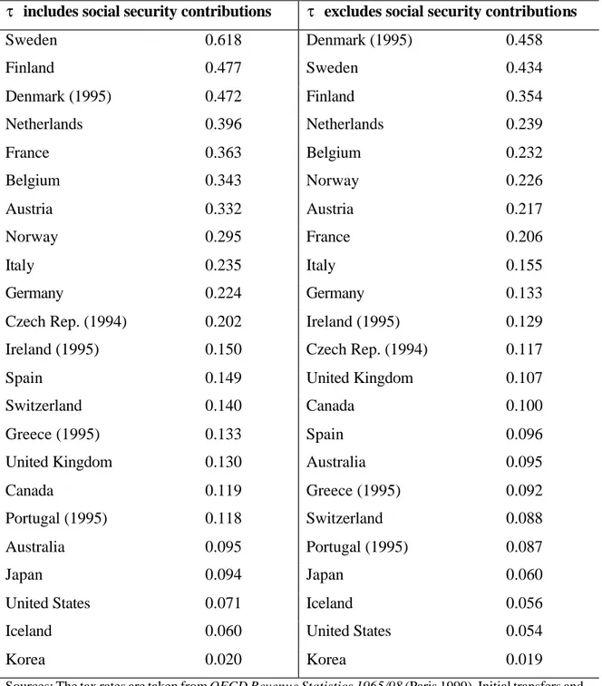
The right-hand side of (17’) – which is always greater than zero because of condition (6b) – contains preference and technology parameters that are difficult to measure, but that can be assumed, as a first approximation, to be equal across countries. We may think of the left-hand side as a transfer-adjusted aggregate tax rate. It contains policy parameters for which we can easily obtain numerical values, which will typically vary widely across countries. A ranking according to this statistic gives an indication of which countries have the highest potential for self-financing tax cuts – provided that all countries satisfy the standard solvency assumption, and that they all follow a steady-state growth path. Unlike an ordinary tax rate, our transfer-adjusted tax rate can be in excess of 100 percent; in the limit, when C0 T0 →1 (think of a socialist economy!), the left-hand side approaches infinity. Conversely, when C0 T0 →∞, the
transfer-adjusted tax rate approaches zero (this is an implication of PROPOSITION 1).
Before looking at the transfer-adjusted tax rates reported in Table 1 below, a few words of caution are warranted. First, the question is whether the AK model can be taken seriously, in the sense that analytical results derived from that model can be regarded as relevant when considering the economies of the real world. This is clearly an open question.11 For instance, the fact that the model abstracts from labor (capital is the only input) seems questionable. On the other hand, it is important to keep in mind that the variable K should be thought of as representing a broad aggregate, including human capital. Since raw labor probably constitutes a small proportion of total factor inputs in developed countries, it is not obvious that the omission of this particular factor is a very serious drawback.
Second, given that one has accepted the model per se, the problem remains of finding reasonable parameter values for it. In the theoretical model, the tax rate τ is well-defined: it is the tax rate on reproducible capital, which is the only factor of production. In the actual world, physical capital is taxed by the corporate income tax as well as by the personal income tax, while human capital is subject to payroll taxes, as well as to personal income taxes. Things are further complicated by the fact that, in a closed economy, the effective tax burden on human capital is mainly determined by the progressivity of the labor income tax schedule, rather than by the average tax rate. For simplicity, we have disregarded all these complications, and we set τ equal to the tax to GDP ratios reported in the OECD Revenue Statistics 1965/98 (Paris 1999).12 There are two measures of the aggregate tax ratio, namely Table 1: Total tax revenue as percentage of GDP”, and ”Table 2: Total tax revenue (excluding social security) as
11
For a vigorous defense of the empirical usefulness of the AK model, see McGratten (1998). 12
We are not the only ones brave enough to reduce the hundreds of special provisions of the actual tax code to one or two flat rate taxes on reproducible factors in a simple growth model; see e.g. Lucas (1990) and Stokey and Rebelo (1995).
percentage of GDP”. Whether social security contributions should be counted as taxes or not depends on whether they are actuarially fair. As this varies over social security systems and over countries, we have made computations using both alternatives when we have analyzed (17’). Initial transfers T and consumption 0 C are taken from the 0 OECD National Accounts 1984-1996, Volume II (Paris 1998). Most figures refer to
1996, but for some countries no later data than 1994 or 1995 were available.
(Insert Table 1 here)
The results are shown in Table 1. We see that the ranking of the countries remains virtually the same, regardless of whether we define τ as including or
excluding social security contributions. The transfer-adjusted tax rate of the countries in the top is 3 or 4 times as large as that of the countries in the middle, and 5-10 times as large as that of the countries at the bottom of the table. The countries with most potential for self-financing tax cuts are the welfare states in Northern and Western Europe. At the other end of the scale, with transfer-adjusted tax rates well below ten percent, we find the United States, Iceland, and Korea, where public transfers are modest fractions of private consumption.
A much more difficult question is whether countries actually are on the downward-sloping segment of the Laffer curve. To answer this question, we need reliable estimates of the parameters A, σ and θ on the right-hand side of (17’). As for
A, Feldstein (1996) reports that the real rate of return to equity in the US has been 9.3
percent per annum. This figure has been criticized for being too high, but since our model can be thought of as including human as well as physical capital, it does not seem entirely unrealistic as a measure of A. On the other hand, Ireland (1994) and
King and Rebelo (1990) use an estimate of A equal to 16.3 percent. In the following we simply assume that A=0.1. There is little empirical ground for choosing a value of θ. Here, we simply set θ =0.02.
As for the intertemporal elasticity of substitution, Ireland (1994), in line with King and Rebelo (1990), set σ equal to unity. As already noted, such a value seems large when compared to available empirical estimates. A number of
macroeconometric studies, see e.g. Campbell and Mankiw (1991), have reported estimates of σ which are close to zero. But when comparing the micro and
macroeconometric evidence, Attanasio and Weber (1993) conclude that the aggregate evidence is biased downward. Their own preferred estimates of the intertemporal elasticity of substitution range from 0.3 (on aggregate British data) to 0.8 (on cohort data). We adopt these figures as our benchmark values for σ .13
When σ =0.3 the right-hand side of (17’) becomes 2.53. If this number is correct, no country in Table 1 is even close of being in the position of enjoying a self-financing tax cut. Sweden comes closest, but its transfer-adjusted tax rate of 0.618 is still much too low. If the left-hand side of (17’) is to be as large as 2.53, given the Swedish aggregate tax rate of 0.519, the ratio of current transfers to private consumption, T0 C0 , needs to be as large as 0.826. This is much above the actual
Swedish transfer rate, which was 0.543 in 1996.
When σ =0.8 the right-hand side of (17’) drops drastically, down to 0.45. Now, dynamic Laffer effects are possible for some countries. When τ includes social security contributions, Sweden, Finland and Denmark would find a tax cut profitable.
13
It might be noted that the parameters that we have chosen produce a range of growth rates that appears to be fairly reasonable. With A =0.1, θ =0.02, σ =0.3 and τ=0.4 –an aggregate tax rate which appears to fit many European countries – the (instantaneous) growth rate is 1.2 percent; when we rather set σ =0.8 the growth rate is 3.2 percent.
When τ excludes social security, only Denmark can enjoy a self-financing tax cut, though Sweden (with a transfer-adjusted tax rate of 0.434) is a borderline case. If we increase σ further, to 0.9 (which is still well within the bounds of confidence found in the cohort estimates of Attanasio and Weber (1993)), the right-hand side of (17’) drops to 0.31, which implies that also countries like the Netherlands, France, Belgium and Austria may enjoy the benefits of a dynamic Laffer effect. It is also of some interest to note that if a low-transfer country like the USA is to enjoy a dynamic Laffer effect, σ needs to be as large as 1.15.
A conclusion to be drawn from this exercise is that the results are very sensitive to the assumptions made. In particular, we need a very precise estimate of the intertemporal rate of substitution to say something trustworthy about the scope for a dynamic Laffer effect. For those who put faith in the macroeconometric evidence suggesting that σ is close to zero, the conclusion seems to be that lower taxes on capital is no free lunch – other taxes need to be raised, either today or tomorrow, to compensate for the dynamic revenue loss. For those who rather prefer the cohort estimates of Attanasio and Weber (1993), suggesting that the intertemporal elasticity of substitution is higher (but still below one), the lesson seems to be that a handful of countries might be in the vicinity of the peak of the dynamic Laffer curve.
6. Conclusions
This paper makes the following points. The concept of a Laffer curve effect is not self-evident in an intertemporal framework. We explore two possible definitions of such effects. The first one assumes that government spending follows some
spending in one period without requiring a lower level of spending in another. The other definition deals with a predetermined ratio of government spending to GDP, and the question is whether a tax cut will permit a higher spending-to-GDP ratio. We show that there can never be any dynamic Laffer effects according to the second definition, while the magnitude of government’s transfers to households play a crucial role for the scope for dynamic Laffer effects according to the first definition. Here, it turns out that the critical variable is not the tax rate per se, but the “transfer-adjusted” tax rate.
Finally, all our analytical results refer to the AK model. An interesting agenda for future research is to systematically study the scope for dynamic Laffer effects in other types of endogenous growth models.
Appendix
This Appendix shows that our main results extend to the case when the utility function in (3) is multiplicative, rather than additive, in C and G. Consider the following utility function, used by e.g. Bruce and Turnovsky (1999):
dt e G C s U η s −θt ∞
∫
= 1( ) 0 , (A1)where −∞<s<1, and η≥0. Moreover, to ensure concavity, we have that ηs<1, and s(1+η)<1. It also follows that s is related to our measure of the intertemporal elasticity of substitution via σ =1/(1−s). Maximizing (A1) subject to (4) gives us the modified Euler equation
) 1 ( ) 1 ( − +η =θ −r −τ G G s C C
s & & . (A2)
Using (A2) it is easy to see how multiplicative preferences affect our analysis of dynamic Laffer effects.
Let us start with the case of DEFINITION 1. Under the assumption that G grows at a predetermined exponential rate γ , we can write (A2) as G
[
τ θ]
σ − − ′ = A(1 ) C C& ,where θ′=θ −ηsγG. Thus, exogenous public consumption growth operates like a
shift factor, which alters the value of the rate of time preference. As a consequence, all the results derived in section 3 carries over to the case of multiplicative utility; the only novelty is that θ is replaced by θ′ in all our derivations.
Let us next consider the case of a dynamic Laffer effect in the sense of DEFINITION 2. In this case the growth rate of G is in fact tied to the growth rate of C;
] ) 1 ( [ τ θ σ′ − − = r C C& , (A3)
where σ′=1(1−s(1+η)). Thus, public consumption growth now operates as an adjustment to the intertemporal elasticity of substitution. As all the other derivations remain the same, the only modification introduced by multiplicative utility is that we have to replace σ with σ′ in inequality (21), which sets the stage for PROPOSITION 3.
References
Attanasio, O. P. and G. Weber, 1993, Consumption growth, the interest rate and aggregation, Review of Economic Studies 60, 631-649.
Bruce, N. and S. J. Turnovsky, 1999, Budget balance, welfare, and the growth rate: “Dynamic scoring” of the long-run government budget, Journal of Money,
Credit, and Banking 31, 162-186.
Campbell, J. Y. and N. G. Mankiw, 1991, The response of consumption to income: A cross-country investigation. European Economic Review 35 (4), 723-67. Feldstein, M., 1996, The missing piece in policy analysis: Social security reform.
American Economic Review 86 (2), 1-14.
Fullerton, D., 1982, On the possibility of an inverse relationship between tax rates and government revenues, Journal of Public Economics 19, 3-22.
Ireland, P. N., 1994, Supply-side economics and endogenous growth, Journal of
Monetary Economics 33, 559-571.
King, R.G. and S. Rebelo, 1990, Public policy and economic growth: Developing neoclassical implications, Journal of Political Economy 98 (S), 126-150. Lucas, R. E., 1990, Supply-side economics: An analytical review, Oxford Economic
Papers 42, 293-316.
Malcolmson, J. M., 1986, Some analytics of the Laffer curve, Journal of Public
Economics 29, 263-279.
McGratten, E. R., 1998, A defense of AK growth models, Federal Reserve Bank of
Minneapolis Quarterly Review 22, 13-27.
Stokey, N. L. and S. Rebelo, 1995, Growth effects of flat-rate taxes, Journal of
Table 1: Ranking of OECD countries with respect to the transfer-adjusted aggregate tax rate, 1 / 0 0 T − C τ
τ includes social security contributions τ excludes social security contributions
Sweden 0.618 Denmark (1995) 0.458 Finland 0.477 Sweden 0.434 Denmark (1995) 0.472 Finland 0.354 Netherlands 0.396 Netherlands 0.239 France 0.363 Belgium 0.232 Belgium 0.343 Norway 0.226 Austria 0.332 Austria 0.217 Norway 0.295 France 0.206 Italy 0.235 Italy 0.155 Germany 0.224 Germany 0.133
Czech Rep. (1994) 0.202 Ireland (1995) 0.129
Ireland (1995) 0.150 Czech Rep. (1994) 0.117
Spain 0.149 United Kingdom 0.107
Switzerland 0.140 Canada 0.100
Greece (1995) 0.133 Spain 0.096
United Kingdom 0.130 Australia 0.095
Canada 0.119 Greece (1995) 0.092
Portugal (1995) 0.118 Switzerland 0.088
Australia 0.095 Portugal (1995) 0.087
Japan 0.094 Japan 0.060
United States 0.071 Iceland 0.056
Iceland 0.060 United States 0.054
Korea 0.020 Korea 0.019
Sources: The tax rates are taken from OECD Revenue Statistics 1965/98 (Paris 1999). Initial transfers and initial consumption are taken from OECD National Accounts 1984-1996, Volume II (Paris 1998). For each country, we have computed the level of transfers from Table 6, ”Accounts for general government, Disbursements”, as the sum of row 26 (subsidies) and row 27 (other current transfers), minus row 35 (transfers to the rest of the world). We have computed consumption from Table 2, “Private consumption by type and purpose”, row 43 (private final consumption expenditure).