Accident cost, speed and vehicle mass externalities, and insurance

Accident Cost,

Speed and Vehicle Mass

Externalities, and Insurance

26

Discussion Paper 2011 • 26

Lars HULTKRANTZ

Orebro University, Sweden

Gunnar LINDBERG

VTI and Centre for Transport Studies, Sweden

ITF/OECD Joint Transport Research Centre Roundtable 151, 22-23 September 2011:

INSURANCE COSTS AND ACCIDENT RISKS

Discussion Paper No. 2011-26

Accident cost, speed and vehicle mass externalities,

and insurance

Lars HULTKRANTZ

Orebro University

Gunnar LINDBERG

VTI and Centre for Transport Studies (CTS) Sweden

September 2011

The views expressed in this paper are the authors’, and do not necessarily represent the opinions of Orebro University, the VTI and Centre for Transport Studies (Sweden),

 

INTERNATIONAL TRANSPORT FORUM 

The International Transport Forum at the OECD is an intergovernmental organisation with  52 member countries. It acts as a strategic think‐tank, with the objective of helping shape the  transport policy agenda on a global level and ensuring that it contributes to economic growth,  environmental protection, social inclusion and the preservation of human life and well‐being. The  International Transport Forum organises an annual summit of Ministers along with leading  representatives from industry, civil society and academia.  The International Transport Forum was created under a Declaration issued by the Council of  Ministers of the ECMT (European Conference of Ministers of Transport) at its Ministerial Session in  May 2006 under the legal authority of the Protocol of the ECMT, signed in Brussels on 17 October  1953, and legal instruments of the OECD.   The Members of the Forum are: Albania, Armenia, Australia, Austria, Azerbaijan, Belarus, Belgium,  Bosnia‐Herzegovina, Bulgaria, Canada, Croatia, the Czech Republic, Denmark, Estonia, Finland,  France, FYROM, Georgia, Germany, Greece, Hungary, Iceland, India, Ireland, Italy, Japan, Korea,  Latvia, Liechtenstein, Lithuania, Luxembourg, Malta, Mexico, Moldova, Montenegro, the  Netherlands, New Zealand, Norway, Poland, Portugal, Romania, Russia, Serbia, Slovakia, Slovenia,  Spain, Sweden, Switzerland, Turkey, Ukraine, the United Kingdom and the United States.   The International Transport Forum’s Research Centre gathers statistics and conducts co‐operative  research programmes addressing all modes of transport. Its findings are widely disseminated and  support policymaking in Member countries as well as contributing to the annual summit. 

 

Discussion Papers 

The International Transport Forum’s Discussion Paper Series makes economic research,  commissioned or carried out at its Research Centre, available to researchers and practitioners. The  aim is to contribute to the understanding of the transport sector and to provide inputs to transport  policy design. The Discussion Papers are not edited by the International Transport Forum and they  reflect the author's opinions alone.  The Discussion Papers can be downloaded from:  www.internationaltransportforum.org/jtrc/DiscussionPapers/jtrcpapers.html  The International Transport Forum’s website is at: www.internationaltransportforum.org  For further information on the Discussion Papers and other JTRC activities, please email:  itf.contact@oecd.org 

Accident cost, speed and vehicle mass

externalities, and insurance

Discussion Paper, September 2011

Lars Hultkrantz*, Gunnar Lindberg**1

* Örebro University, **VTI and Centre for Transport Studies (CTS)

1 Introduction

Traffic accidents are a human tragedy that kills 1.2 million people worldwide annually (World Health Organization, 2004). The cost of traffic accidents are huge and recent estimates for US alone suggest the cost to be USD 433 billion in year 2000 or 4.3 percentage of GDP (Parry et al, 2007). A reduction of this cost can be done in two ways, either by reducing the number of accidents or by mitigating the consequences of the existing accidents. Insurance systems can contribute to both.

Vickrey (1968) suggested a partial solution to problems of unaffordable insurance, uninsured driving, premium unfairness and inefficiencies by proposing usage-based car insurance. In fact, several insurance companies have now adopted Vickrey’s idea in the form of Pay-As-You-Drive (PAYD) automobile insurance (Bordoff and Noel 2008). This policy enables insurers to charge the vehicle owner per mile instead of a pre-set number of miles per year. PAYD is offered to motorists on an optional basis, i.e., they can also choose a conventional scheme.2

PAYD insurance builds on the improved possibilities brought by new in-vehicle technologies for measuring distance driven. However, there is a range of other risk factors that could be

supervised, some of which are already used by the insurance industry. For instance, one Swedish insurance provider charges a lower premium to vehicles that have an alco-lock installed to make it impossible to use the vehicle for an intoxicated driver. In this report, we summarize some work we have done on how to incorporate two of the most important risk factors; vehicle mass and speed.

The possibility to differentiate insurance premiums according to various risk factors raises questions on the interaction between vehicle insurance schemes and taxes. Distance driven,

      

1

We are grateful to our colleagues and co-authors Sara Arvidsson, Lina Jonsson, and Jan-Eric Nilsson who participated in the studies summarized here.

2

Another possibility is annual odometer audits. However that would probably be much more costly than electronic measurement of distance (Bordoff and Noel, 2008).

speeding and vehicle mass are in many countries subject to taxation (for instance gasoline tax for distance, speeding tickets for speed and vehicle tax for vehicle mass). These kind of taxes can be thought of as (often imperfectly implemented) Pigou taxes levied by a principal (a state regulator) that wants to control agents (motorists) that cause various externalities. Insurance companies are then another principal influencing these agents. As the state and the insurance companies have different objective functions and are subject to different legal, informational and technological constraints, taxes and insurance programs are imperfect substitutes as instruments for influencing road traffic safety. In section 2 we will briefly discuss how a PAYD scheme with a speeding penalty (this will here be called Pay As You Speed, PAYS) can be combined with taxes to implement a Pigou taxation of road accident externalities. PAYS vehicle insurance is designed to affect speed, which is a main risk factor that affects the number of accidents as well as the severity of accidents. In section 3 we summarize results from a vehicle-fleet experiment with a PAYS insurance incentive for keeping within speed limits using a speed-alert device. The PAYS scheme was simulated with a monthly bonus to participants during two months reduced by a non-linear speeding penalty. Participants were randomly assigned into four treatment and two control groups. A third control group consisted of drivers who had the device and were monitored, but did not participate. We found that participating drivers reduced severe speeding during the first month, but in the second, after having received feedback reports with an account of earned payments, only those that were given a penalty changed behaviour.

In sections 4 and 5 we turn to another major risk factor; vehicle mass. Vehicle mass is a crucial factor for the distribution of injuries between occupants in involved vehicles in a two-vehicle crash. A larger two-vehicle mass protects the occupants in the two-vehicle while on the same time it inflicts a higher injury risk on the occupants in the collision partner vehicle. In section 4 we analyse this “mass externality” using a database including collision accidents in Sweden involving two passenger cars during five years. In each accident the two involved vehicles are divided into the lighter vehicle and the heavier vehicle and the effect of weight is examined separately for the two groups. We find that the accident costs that fall on the lighter vehicle increases with the mass of the heavier vehicle and decreases with its own mass. Given that a vehicle is the heavier one in the crash, neither the own mass nor the mass of the lighter vehicle significantly affect the accident cost. The expected external accident cost is calculated and it is shown to increase rapidly with vehicle mass.

Section 5, finally, uses the results from the previous section to discuss different solutions to internalization of this external accident cost. We calculate a mass dependent multiplicative tax on the insurance premium in a no-fault insurance system.

Sections 2 and 3 on PAYS insurance are brief summaries of studies that will soon be published, and therefore can be read in full length elsewhere, while sections 4 and 5 on differentiation with respect to vehicle mass present more novel results and will therefore be presented more extensively.

2 Taxes

on

accident

externalities and PAYS insurance

In Hultkrantz et al. (2011) we suggest a design of Pigou taxation in combination with PAYS insurance in order to internalize road accident externalities. We describe a setting involves two principals (the state and an insurance company) that affect the economic incentives of motorists for driving and for driving carefully. While the state regulator is assumed to aim for overall social efficiency by implementing full marginal cost pricing, the insurance company make use of actuarial pricing to cover their costs, i.e. average cost pricing within risk classes that they

estimate to be homogenous. Since insurance companies have means for differentiation across risk classes that are not available to the government, the insurer can be an agent for the regulator’s traffic safety policy. Another specific feature of this setting, in contrast to conventional Pigovian taxation, is that differentiation can be accomplished by self selection. Therefore, compulsory regulation is not necessary.

For this aim, we use a modal-mix model to analyze the accident externalities from car driving and from speeding. The risk of collisions is the source of a reciprocal externality within the group of motorists, as every driver is increasing the accident risk of all drivers by just being on the road, and even more so if he or she is speeding. However, the distribution of these external effects is also affected by cross-subsidization by fiscal means, since some accident costs such as medical care are paid for through taxes, and through vehicle insurance (as different categories of drivers with different accident risk cannot, in the absence of PAYS insurance, be separated). The model we use comprises commuters who have a choice between a car mode and a reference travel mode. Motorists may also choose to comply or not to comply with speed limits; hence the model has three modes distinguished by speed (and therefore also time to get to destination) as well as accident risk. With this model we show how the cost burden of automobile accidents is spread between non-motorists and motorists with different risk profiles. Further, we use the model to show how the modal mix, i.e., the driving and speeding decisions, are affected by a change from conventional to PAYS insurance, and, with conventional insurance, by a tax on vehicle insurance premiums.

We derive Pigovian price equations for a complete internalization of car accident externalities with two sets of instruments; first a conventional solution that combines two taxes, a tax on driving (vehicle usage) and a tax on speeding (speeding tickets), and second a solution with PAYS insurance and a tax on vehicle insurance. It is thus necessary to use two separate policy instrument since it is important not only to induce roads users to drive at legal speeds but also to strike an optimal balance between whether to use the car mode or not. Using these price

equations a numerical example, calibrated on Swedish data, indicates that the standard Pigovian tax solution would require very high speeding charges, while the PAYS insurance could come close to a full internalization without any substantial change of the level of vehicle taxation in comparison to the current situation. In Sweden, there already exists a 32 percent tax on the compulsory part of the vehicle insurance.

While the external costof driving cars in non-congested areas in Sweden seems to be already internalized by the current fuel tax, the external cost of speeding is only to a very small extent internalized by the expected cost of speeding tickets. In fact, with PAYS insurance taxes can be

designed so as to reduce the role of speeding tickets.3 Hence, the system would mean that speeders – who by assumption are not inclined to install the equipment – could continue their behavior and get away with it by paying a higher insurance premium. While this could be interpreted as a mechanism for paying for the right to speed, the main difference compared with today would be that people currently speed without having to pay (fully) for it.

A caveat is, however, that vehicle insurance is assumed to be compulsory and that all drivers actually pay. However, even when vehicle insurance only has to cover material vehicle damages, and even in a country with such law-obeying motorists as in Sweden, a fraction of the cars are driven without any insurance (and/or without paying vehicle taxes). That proportion would likely increase if insurance fees were raised. The use of vehicle insurance to internalize the full social cost of accidents would thus in a way transform the traffic surveillance problem from detection of speeding to detection of non-insurance. However, as monitoring of non-insured vehicles is as a rule considerably more easy than monitoring of speeding we regard this as a minor objection.

3 Moral

hazard

reduction

with PAYS insurance – the

Swedish vehicle fleet economic experiment

In 2002, we conducted an economic experiment of a PAYS insurance scheme using 114 motorists in the city of Borlänge, Sweden, that had participated in a technological trial of a speed alert (“Intelligent Speed Adaptation”, ISA) system based on in-vehicle GPS recording of vehicle speed and position. The study is reported in Hultkrantz and Lindberg (2012). Later similar studies have been made in Denmark (Agerholm et al. 2008) and the Netherlands (Bolderdijk et al. 2011). Here we briefly summarize our own study.

The focus of our study is on moral hazard effects among users, not on selection effects. We study how some features of a PAYS scheme, the magnitude of a participation bonus and a penalty fee, affect driving behaviour of those drivers that have accepted to participate. Our field experiment was designed for the purpose of evaluation of a PAYS insurance based on ISA equipment. A vehicle-fleet trial is very costly but we were given an opportunity to use an already existing fleet trial. Vehicles for this trial had been recruited through an offer to a random sample of 1000 private car owners in a Swedish city (Borlänge, pop. 48 000) to get ISA equipment installed free of charge. No other economic incentives were used in this trial. 250 private car owners accepted to have their vehicles provided with on-board computers with digital maps, GPS positioning and mobile communication facilities. The technical system informed the driver about the speed limit on a display in the vehicle while an acoustic signal and a flashing light alerted him or her if the vehicle was driven faster than the speed limit (Bergeå and Åberg 2002).

The original trial was completed in December 2001. Early next year, the car owners were informed that they could keep the equipment for some time if they wanted. During the late

      

3

As long as the PAYS insurance is voluntary some need for external speed monitoring remains because otherwise those who stick with conventional insurance will speed even more than presently.

spring, we invited 114 private car owners that still had these devices installed to participate in an economic experiment for two months (September and October 2002).These months were chosen for the main experiment, because they are free from the two major seasonal

“distortions” in this part of Sweden:, that is, summer vacations (from mid June to mid August) and winter road conditions (November – March), both having major effects on aggregate travel and speeding patterns. After the second experiment month was completed, however, we had not exhausted the project budget so we offered the participants to continue for a third month. As will be shown later, that turned out to be of no use since winter came during that month.

Car owners were informed that they would receive a monthly bonus of 250 SEK or 500 SEK to be paid immediately at the end of the month and that this bonus would be reduced by a penalty each minute they drove faster than the speed limit4_{. The size of the penalty varied in}

four steps, depending on the magnitude of speed violations, between 0 and 1 SEK per minute, or between 0 and 2 SEK per minute5_{. All participating drivers, also those that would get the}

lump-sum bonus without penalty reductions, got individual feedback reports on their total time of driving and speeding, together with the monthly bonus payment.

Those owners that accepted to participate were randomly assigned to a high or low initial bonus (250 SEK/month or 500 SEK/month), and to the three penalty categories (zero penalty; 0 – 1 SEK/minute; and 0 – 2 SEK/minute; respectively). To always make participation beneficial in monetary terms, a cap was introduced to the total penalty charges so that even high offenders would get a net payment of at least 75 SEK each month. As it later turned out, no one was even near of hitting this ceiling.

A majority of the car owners (95 persons out of 114) accepted to participate in the

experiment, while nine drivers rejected, and ten did not respond. Drivers that accepted were hence randomly divided into six groups as shown in Table 1. There were 16 drivers in each of the groups A-E and 15 drivers in group F.

A remaining group (G) consisted of the 19 drivers that rejected or did not respond to the offer to take part in the economic experiment. These non-participators were still using the

equipment and had been informed that their driving would be continued to be monitored for research purposes. This give us opportunity both to cast some light on self-selection effects and to have a control group, although not randomly selected, with zero bonus, zero penalty, and no individual feedback reports.

      

4

Speeding is recorded and summed over month in seconds. For penalty this is rounded downwards to whole minutes.

5

Table 1. Treatment groups (participants)

Zero penalty Low penalty level (0-1 SEK/min)

High penalty level (0-2 SEK/min) High bonus (500 SEK) A C E

Low bonus (250 SEK) B D F

The four-step penalty scheme was progressive to reflect that accident risk increases

progressively with the speed of the car (Nilsson 2000). The levels of the low penalty charge were set so as to correspond to the estimated external cost of speed choice, according to a cost-benefit model used by the Swedish National Road Administration. Hence, since the technical speeding detection probability is one (or close to one), this penalty scheme approximates a pure Pigou fee on speeding.

Those given the low penalty scheme were charged 0.10 SEK per minute when the actual speed exceeded the speed limit by 0-10 percent, 0.25 SEK per minute when speed was 11-20 percents above limit and 1.00 SEK per minute for speed offences above 20 percent. Those car owners that were given the high penalty scheme were charged twice as much.

The experimental design makes it possible to control for a variety of effects. First, the non-participating group G offers control over effects on speeding evoked by external factors, such as change of weather conditions. Second, the zero-penalty groups A and B control for

Hawthorn effects from being participator in an experiment, in which every participant is given feedback information on his/her own driving behaviour. Third, the two bonus levels control for income effects, or other possible effects from the size of the participation bonus.6 Finally, the two penalty levels make it possible to evaluate both the effect of penalties vs. no penalties (comparing C and E to A, and D and F to B) and to effect of the size of penalties (comparing C to E and D to F). However, it must be borne in mind that the experiment groups are small. Also, unfortunately, due to technical failures of some equipment we lack some reference driving data, in particular for October 2001.

Data records were automatically collected once a month through mobile communication. The data contains information on geographical X- and Y-coordinates, time and date. This

information was recorded frequently (every tenth second) as long as the car engine was running. The data is summarized as individual speed profiles for each road type (defined as roads with different speed limits). As the technology was known from the technical trial to have some flaws, data was filtered from outliers to protect drivers from erroneous charging. At the end of each period, the participants received information about their speeding behaviour, the sum of penalty charges and the remaining net bonus.

      

6

In behavioural economics, a general observation is that many people behave in a reciprocal manner (Rabin 1993) including the phenomenon of “conditional cooperation” (Fehr and Fishbacher 2002), that is, that people contribute (to a common good) contingent upon others contribution. This could imply that drivers that were given the high participation reward would contribute more (high compliance to speed rules). Another possible effect of bonus size comes from “corner effects”, that is, that a driver with low bonus is more close to the penalty cap (SEK 75) where the marginal cost of further speeding is zero.

In the individual feedback reports to the participants, speed violations were divided into three severity classes; Minor (0-10%), Medium (11-20%) and Major (≥ 21%). The reports stated the total time (minutes) during one month (t) that the car (i) had been driven faster than the speed limit, in total, and within each severity class, By dividing these variables with the total travel time of the car during the same month, we computed speeding frequencies; measuring the proportion of total travel time that the car is used for driving faster than the speed limit, in total and within each severity class.

In evaluating the results, we did paired-difference tests, comparing across groups the

difference of the outcome variable during one of the experiment months with the level of the same variable during a reference month, which here will be the same month one year before. Thus, for drivers for which we have all observations, we compared the levels of the outcome variables in September and October 2002, respectively, to these levels in September and October 2001, respectively. However, since our sample is small, and is further reduced by lack of observations for some drivers in 2001, especially in October, the evaluation of results was based on regressions, using observations of all individuals, and controlling for individual covariates, that is, not on comparison of group by group averages.

3.1 Results

The average participating car owner (Group A-F) was 57 years old and had an annual income of SEK 384 000. The participants were therefore on average older and had higher income than the car owners in general.7 26 percent were female (national average is 31 percent). Non-participants (Group G) were on average 5 year younger and had an even higher income than participants, but only the age difference to participants is statistically significant.

Participants on average drove faster than the speed limit around 14 percent of the driving time, while non-participants were on average speeding 17 percent of the driving time. This difference is, however, not significant. For Severe speeding, the proportion of driving time was 4 percent for participants and 6 percent for non-participants. This difference is significant at the five percent level. However, the significance disappears in a regression controlling for the individual covariates (Sex, Age, Age squared, and Income).

Table 2 shows the final estimated models (after subsequent reductions following a general-to-specific procedure) estimated for one-year differences of Severe speeding in the two monthly samples for September and October, respectively. The sample sizes are mainly restricted by limited number of observations of driving (speeding) behaviour in 2001, which leaves 81 and 48 observations in the two samples, respectively. There also are a few observations of the income variable missing. As shown, for the September difference, two variables, Age and Participation, remain in the reduced model; together explaining 12 percent of the total

variation. In the reduced October difference model, the three remaining variables are Penalty, Sex and Income*Sex; explaining 47 percent of the total variation.

      

7

The average age of a car owner in Sweden is approximately 46 years (SIKA 2006). The average annual income of full time employees in 2001 was SEK 295 000.

The regression results show that subjects of all treatment groups reduced Severe speeding during the first experiment month, while only subjects in groups that were given speeding penalties reduced Severe speeding during the second month. No other treatment variables (or interactions, not shown) were significant.

During the economic experiment participants significantly reduced their speed violations compared to non-participants. The time proportion of speed violations was reduced from around 15 percent of total driving time prior to the experiment to between 8 percent and 5 percent during the experiment with the lower interval at the end of the experiment period. Non-participants had almost constant proportion violations during the experiment.

During the first experiment month the priced participants reduced the speed violations more than the zero-penalty participants but the difference was not significant. However, during the second month priced participants reduced severe violations significantly more than the zero-penalty group; the former had a reduction of 64 percent while the latter only had a reduction of 15 percent. As mentioned, the regression analysis gives statistical evidence of a participant effect in September and a penalty effect in October. This implies that a penalty charge is essential for having a lasting effect on severe speeding, that is, the “placebo” or “Hawthorn” effects of participation that seem to be present in the September sample is not statistically significant in October.

The results do not indicate any difference between the two penalty charge levels. This suggests that drivers have had a binary decision, either to change or not to change their regular behaviour, and that, at least for the duration of our experiment, the low level was high enough to exhaust the potential for that. This further suggests that a simpler scheme than the four-tier penalty rate we used would suffice, for instance a flat charge per minute for speed violations exceeding the speed limit by a certain margin. Finally, there was no significant behavioural difference between groups with different bonus levels.

In conclusion, our study thus suggests that economic incentive schemes, in the form of insurance programmes or otherwise, coupled to the use of speed monitoring devices may be an effective way of reducing severe speeding, and thereby to increase overall road-traffic safety. The results imply that even drivers that voluntarily have installed such devices in their cars may be highly sensitive to economic incentives.

Table 2. OLS estimation results for one-year differences of Severe speeding in the September

and October samples, respectively. Base (general) and reduced (specific) models. Standard errors within parentheses.

Variable September 01-02 October 01-02

Base Reduced Base Reduced

Constant -0.025 (0.045) 0.015 (0.014) -0.053 (0.070) -0.001 (0.006) Participation 0.025** (0.011) 0.026*** (0.009) 0.009 (0.018) Penalty 0.004 (0.008) 0.018 (0.012) 0.021** (0.008) High penalty -0.002 (0.008) 0.005 (0.013) High Bonus -0.001 (0.007) 0.004 0.010 Sex 0.0003 (0.0075) 0.032*** (0.011) 0.062*** (0.013) Age 0.001 (0.002) 0.002 (0.003) Age-squared -0.000015 (0.000015) -0.00002 (0.00002) Income 0.000005 (0.000012) -0.000037** (0.000015) Income*Sex -0.000061*** (0.000018) R-squared 13.8 11.8 43.0 47.2 Numb. Obs. 79 81 47 47

4 Vehicle mass and accident cost

Elvik (1994) classified the external cost in three components; the externality generated by changed accident risk due to higher traffic volume (traffic volume externality); the cost for the rest of the society in form of general health care etc (system externality) and thirdly, the increased risk a car driver imposes on other drivers and road user categories, such as pedestrians and cyclists (traffic category externality). The last component is in this section further refined and analysed as an externality between different car sizes. In the next section we discuss how a Pigou scheme could be designed to correct for this externality, using a combination of taxes and vehicle insurance.

The change in velocity that a vehicle experiences in a collision is a good measure of the severity of the crash and works as a predictor of the fatality and injury risk (Toy and Hammit, 2003). In a two vehicle collision where the vehicles move in the same or opposite directions, the change in velocity is a function of the masses of the involved vehicles and their initial

velocities according to equation 1 where m are the masses of the vehicles and v are their initial velocities8.

(

i j

)

j i j i _{m m} v v m v + + = Δ (1)

The velocity change will be greatest for the lighter vehicle which thereby also has higher fatality and injury risk. As the equation above shows, an increase in own mass will both lead to a lower velocity change for the own vehicle and a greater velocity change for the collision partner. Increased mass will thereby improve the vehicle’s crashworthiness while in the same time increase the aggressivity.

Besides change of velocity also mean and peak acceleration works as crash severity

parameters (Stigson, 2009). While velocity change is a function of the masses of the involved vehicles the acceleration is also influenced by the vehicle structure, e.g. stiffness. The

literature on vehicle crashworthiness versus aggressivity has to a large extent been focused on the difference between passenger cars and light trucks (Andersson, 2008). Apart from the larger mass of Sport Utility Vehicles, Vans and Pickups, their stiffness and different geometry compared to passenger cars contribute to more severe injuries and fatalities to the occupants in the collision partner (Gayer, 2004; Joksch, 1998; Toy and Hammitt, 2003; White, 2004). Our study focuses on the mass dimension and will thereby ignore the related influence of stiffness and geometry when analyzing the division of the accident cost between the involved vehicles.

The fact that the mass of a vehicle affects the injuries and fatalities in the collision partner implies that there is an external effect of vehicle mass that could be internalized to reach economic efficiency. Without internalisation, the driver will choose vehicle mass based only on the own beneficial effect of mass and ignore the disadvantageous effect on the injury risk in the collision partner.

4.1 Model and data

Accidents are assumed to be bilateral, i.e. they involve two vehicles. The accident probability (A) depends on the level of active care each driver takes and the annual driven distances. The severity of the accident in vehicle i is represented by λi where λi is a function of the traffic environment, occupant characteristics and vehicle characteristics including the masses of both involved vehicles, (zi,zj). It is assumed that δλi/δzi<0, δ2λi/δ2zi >0 while δλi/δzj> 0 and δ2λi/δ2zj

>0. A larger vehicle mass decreases the injuries in the own car but at the same time increases the injuries and thereby the accident cost that falls on the occupants in the collision partner. This is in concordance with the influence mass has on the velocity change in the involved vehicles (eq. 1).

The accident cost consists of economic losses l in form of medical cost and lost income and grief and suffering g. The total accident cost that falls on vehicle i is expressed as λi(g+l). All

      

8

medical cost is assumed to be covered by the driver through full regress including regress from the social security system. Economic losses (l) are assumed to be fully insured. In a strong no-fault system no potential liability to cover the other driver’s loss occurs. The insurance premium for driver i will be:

(

e

)

l A _i

i =

λ

1+

π

(2)

where e is the administrative cost of the insurer as a proportion of the expected loss. Drivers are expected to be risk averse and maximize their expected utility with the utility function U(W,z,π) where ∂U/∂W>0 and ∂2_U/∂2_{W<0. Insurance is assumed to be available at}

actuarially fair rates. Two possible states are assumed, state of accident with a probability of A and a state where no accident occurs with a probability of 1-A. In case of an accident the wealth (W) will be reduced by the accident cost due to grief and suffering while the economic loss is covered be the insurance. The expected utility of driver i can be expressed as:

(

)

i

(

i i

)

z i i

i AW AW g Pz

EU = 1− + −

λ

− −

π

(3)

where Pz is the price of mass, for example through higher fuel consumption. The first order condition for the choice of optimal level of vehicle mass for driver i gives:

( )

(

1

)

_⎥− =0 ⎦ ⎤ ⎢ ⎣ ⎡ + ∂ ∂ + ∂ ∂ − = ∂ ∂ z i i i i i i _{l e P} z g z A z EU λ λ (4)

and it can easily be verified that the second order condition holds. A larger vehicle mass will benefit the driver and passengers through a lower injury risk that is reflected both in a lower expected cost due to grief and suffering (g) and a lower insurance premium as the expected economic loss (l) will decrease. These benefits will be weighed against the cost of mass in the private choice of vehicle.

It is well known that a no-fault system will generate a lower level of care than a tort system (Cummins et al, 2001). The level of care with a no-fault system will be lower than the optimal level. Besides this, a no-fault system will also lead to a choice of vehicle mass that is higher than the social optimum if vehicle mass decreases the injury risk in the own vehicle and increases the injury risk in the collision partner. Assuming a society of two drivers the following first order condition for the first driver’s social optimal choice of vehicle mass can be derived:

(

)

₍

₎

0 ) 1 ( 1 _ _ = ⎥ ⎦ ⎤ ⎢ ⎣ ⎡ + ∂ ∂ + ∂ ∂ − − ⎥ ⎥ ⎥ ⎥ ⎦ ⎤ ⎢ ⎢ ⎢ ⎢ ⎣ ⎡ + ∂ ∂ + ∂ ∂ − = ∂ + ∂ 4 4 4 4 3 4 4 4 4 2 1 4 4 4 3 4 4 4 2 1 y Externalit Negative i j i j z Benefit Internal i i i i i j i e l z g z A P e l z g z A z EU EU λ λ λ λ (5)

In a no-fault system the choice of vehicle mass will be made considering only the internal benefit of a large mass while the increased injury risk to other road-users will be ignored. The dataset includes all police reported personal injury accidents involving exactly two passenger cars in Sweden during 1999 to spring 2004. The dataset consists of information on the conditions at the occasion of the accident including speed limit, weather condition and information on involved vehicles including their mass (both total weight and kerb weight), model and existence of airbag9. The dataset also includes information on the driver and passengers of the vehicles, their sex, age and their injuries if any. The injuries are categorised in three categories; slight injury, severe injury and fatality. Table II presents descriptive statistics.

To construct a common unit for the accident cost the official Swedish valuation for fatalities, severe and slight injuries (SIKA, 2008a) in Table I is used. The valuation is split into material cost including mainly medical cost and lost production (l) and the risk valuation which we take equal to the pain and suffering loss (g). For each accident the total accident cost is calculated and attributed to the vehicle in which the victims where travelling. Since all injuries are categorised in only three levels, the accident cost attributed to the vehicles will in our dataset not be fully continuous but takes only a few values depending on the number of injured occupants and the category of their injuries.

Table I – Valuation of accidents (SEK))

Material cost (l) Risk Valuation (g) Total (l+g) Fatality 1 321 000 21 000 000 22 321 000 Severe Injury 661 000 3 486 000 4 147 000 Slight Injury 66 000 133 000 199 000 1 SEK ≈ 10 Euro cent. Note: Material cost includes only net lost production

For each accident the lighter of the two vehicles is labelled vehicle 0 and the heavier labelled vehicle 1. Table II shows that the average total cost due to injuries and fatalities is higher in the lighter vehicle in spite of the higher average number of passengers (including the driver) in the heavier vehicle. This is a result of the more than twice as many fatalities in the lighter vehicles.

      

9

The original dataset included a few vehicles with a mass above what is normally recognized as passenger cars. Accidents including vehicles with a total weight exceeding 3000 kg have therefore been excluded from the dataset, thereby reducing the number of accidents with 4.

Table II – Descriptive statistics

Lighter vehicle Heavier vehicle Mean N Mean N Age of driver 40.75 3872 41.03 3878 Male driver (yes=1) 0.63 3870 0.67 3880 Number of passenger 1.38 3890 1.40 3890 Young male driver <25 (yes=1) 0.16 3870 0.13 3878 Number of elder passengers (>60) 0.27 3890 0.30 3890 Speed limit (km/h) 65.11 3719 65.11 3719 Age of car 1989.95 3391 1991.60 3159 Kerb weight (kg) 1183.24 3890 1443.45 3890 Total weight (kg) 1554.21 3890 1858.64 3890 Airbag (yes=1) 0.09 3890 0.16 3890 Fatalities 0.02 3890 0.01 3890 Severe injuries 0.18 3890 0.16 3890 Slight injuries 1.09 3890 1.13 3890 Total material cost (SEK) 219 836 3890 190 719 3890

Total accident cost (SEK) 1 425 900 3890 1 080 580 3890

 

4.2 Internal benefit and external cost of increased mass

Given that an accident occurs we are interested in how the characteristics of the different vehicles affect the injuries and thereby the accident cost and how this cost is split between the involved vehicles. Separate models are being estimated for the total cost of fatalities and injuries in the lighter vehicle and the cost in the heavier vehicle as a function of the kerb weights of the involved vehicles10_{. The measure of cost in one vehicle is thus influenced by}

the other vehicle. Earlier studies (White, 2004; Evans, 2001; Fredette et al, 2008) have examined how vehicle characteristics influence the probability for fatalities or severe injuries given an accident. We, instead, estimate the impact of vehicle characteristics on accident costs, so obtaining a more direct measure of the external costs associated with vehicle mass. For the accident costs of the lighter vehicle, we estimate the following linear model:

ε ν δ γ β β α+ + + + + +

= Mass Mass A N . SpeedRestriction

TC_{0 0 0 1 1} irbag₀ oofPassengers₀ (6)

The dependent variable is the total cost of fatalities and injuries λ0(l+g) in the lighter vehicle given a collision with a heavier vehicle. We model the accident cost in the lighter vehicle as a function of the lighter vehicle’s own kerb weight, the kerb weight of the heavier vehicle, the numbers of passengers in the lighter vehicle, the speed restriction at the place of the accident and a dummy for if the lighter car was equipped with an airbag. In an extended model

      

10

It is not self-evident whether the kerb weight (vehicle weight including fuel and a driver at 70 kg) or the total weight (kerb weight and maximum allowed load) best reflects the actual mass of the vehicle at the accident. Both mass variables have been tested and the effect on the premium tax is not affected by the choice.

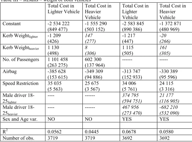
dummies for if the driver is a male between 18 and 25 in the lighter car and the heavier car respectively is added together with variables measuring the sex and age of all the passengers in the lighter car. Vehicle age does not explain the accident outcome and is therefore excluded from the models. Results for both models are presented in Table III.

As expected, the cost will be reduced with vehicle mass for the lighter vehicle and increased with the mass of the heavier vehicle. The number of passengers in the car as well as the speed limit increases the cost. Existence of an airbag decreases the cost. The own mass will reduce the cost for the lighter vehicle with around 1209 SEK per kilogram while every extra kilogram of kerb weight of the heavier vehicle will increase the cost imposed on the lighter vehicle by around 1130 SEK, a cost that is external to the heavier vehicle. We include dummies for male drivers between 18 and 25 for each of the vehicle types, as a proxy for the actual speed at the time of the accident. We also include separate variables for different age groups and for gender so that accident costs can differ among the groups, e.g. because the elderly are more fragile. These dummy variables do not change the conclusions.11

Estimating the corresponding models for the cost of the heavier vehicle gives a quite different result. For the heavier vehicle the cost due to injuries and fatalities is not significantly affected by either the own mass or the mass of the lighter vehicle.

ε ν δ γ β β α+ + + + + +

= Mass Mass A N . SpeedRestriction

TC_{1 0 0 1 1} irbag₁ oofPassengers₁ (7)

      

11

The logic behind the driver dummy is the lack of information in our dataset on actual speed of the vehicles at the time of the accident. Including a dummy for if the driver is a man aged 18 to 25 is an attempt to capture the suspicion that young men drive faster than other groups and correct for this under the assumption that young men are overrepresented in certain vehicle and accident types. Neither the driver dummy for the driver of the lighter nor the heavier car is significant.

Table III – Results – weight of both vehicles Total Cost in Lighter Vehicle Total Cost in Heavier Vehicle Total Cost in Lighter Vehicle Total Cost in Heavier Vehicle Constant -2 534 222 (849 477) -1 555 290 (503 152) -2 583 845 (890 386) -1 372 871 (480 969) Kerb Weightlighter -1 209

(426) 147 (277) -1 217 (447) -20 (266)

Kerb Weightheavier 1 130

(498) 8 (306) 1 115 (505) 161 (305) No. of Passengers 1 101 458 (263 275) 602 300 (137 964) --- --- Airbag -385 628 (153 615) -349 309 (94 886) -313 747 (152 933) -330 389 (95 596) Speed Restriction 35 035 (5 563) 25 675 (3 567) 34 006 (5 761) 24 115 (3 316) Male driver 18-25lighter ---- --- 374 795 (594 751) 21 177 (116 905) Male driver 18-25heavier ---- --- 467 956 (273 470) -682 210 (532 090)

Sex and Age var. NO NO YES YES

R2 0.0562 0.0445 0.0678 0.0580 Number of obs. 3719 3719 3692 3692

Robust standard errors in parentheses; Results non-significant at the 5 % -level in italics Models where the costs in the involved vehicles are estimated as functions of the mass difference instead of the kerb weights themselves are presented below (Table IV). The kerb weight difference is both expressed as the actual difference in kg between the heavier and the lighter vehicle and as the ratio between the heavier and the lighter vehicle.

Table IV – Results – weight difference Total Cost in Lighter Vehicle Total Cost in Heavier Vehicle Total Cost in Lighter Vehicle Total Cost in Heavier Vehicle Constant -2 634 927 (638 525) -1 359 272 (323 172) -2 837 669 (645 711) -937 447 (330 526) Mass1-Mass0 1 165 (418) -63 (256) --- --- Mass1/Mass0 --- --- 822 778 (302 833) -94 862 (187 842) No. of Passengers 1 101 151 (263 344) 603 857 (137 945) 868 453 (204 912) 476 433 (105 881) Airbag -394 239 (147 240) -334 367 (94 129) -291 134 (112 374) -255 842 (71 108) Speed Restriction 35 022 (5 556) 25 697 (3 568) 27 101 (4 334) 19 722 (2 763) R2 0.0561 0.0444 0.0565 0.0453 Number of obs. 3719 3719 3719 3719

Robust standard errors in parentheses, Results non-significant at the 5 % -level in italics The model where the mass difference is expressed as a ratio instead of an absolute difference is harder to give an intuitive interpretation to, but is a common measure in the literature (Evans 2001, Toy and Hammit 2003, Joksch et al 1998). The estimates of the number of passengers, the speed restriction and the airbag are almost constant across specifications. The mass difference – expressed as a difference in kg or a ratio – is highly significant for the cost of the lighter vehicle but not for the cost of the heavier vehicle. Models have been estimated including also the absolute mass of one of the vehicles resulting in insignificant estimates for the vehicle mass variable given the mass difference; i.e. given the mass difference the vehicle mass per see will not influence the consequences of an accident.

Our model thus suggests that minimizing the mass difference in the fleet would be beneficiary while our result supports neither downsizing nor upsizing. This is in contrast to the results in Buzeman et al (1998) that concluded that a uniform mass increase would lower the number of fatalities and Evans (2001) that concluded that in any two-car crash a replacement of both cars with other heavier cars by either a fixed percentage or a fixed amount will reduce the total fatality risk.

4.3 The expected external accident cost

Increasing the mass of a vehicle both increases the probability to be the heavier vehicle in a collision and the expected mass difference given a collision with a lighter vehicle. Both these effects affect the expected accident cost in the collision partner. An increased mass also affects the expected internal accident cost. Since the effect of vehicle mass differs depending

on if the vehicle collides with a heavier or a lighter vehicle the expected costs is the sum of the expected cost given a collision with a heavier vehicle and the expected cost given a collision with a lighter vehicle weighted with respectively probabilities (eq. 8 and 9). Expected External Accident Cost

(

)

(

) (

)

(

(

)

)

(

)

(

(

)

)

(

)

1

(

)

0 ) 1 ( ) 1 ( ) 1 ( TC z z P TC z z P z z e l g z z P z z e l g z z P e l g E j i j i j i j j i j i j j i j > + < = > + + > + < + + < = + + λ λ λ (8) Expected Internal Accident Cost

(

)

(

)

(

)

(

(

)

)

(

)

(

(

)

)

(

)

0

(

)

1 ) 1 ( ) 1 ( ) 1 ( TC z z P TC z z P z z e l g z z P z z e l g z z P e l g E j i j i j i i j i j i i j i i > + < = > + + > + < + + < = + + λ λ λ (9) We use the estimated models excluding driver dummy for the total accident cost from Table III (column 2 and 3) using mean values for speed restriction, airbag and number of passengers for the lighter and heavier vehicles respectively. For each vehicle the mean mass of all

vehicles with a mass exceeding or below the mass of the vehicle in question is used as the mass of the collision partner. The probability to collide with a heavier/lighter vehicle is calculated as the proportion of vehicles in our dataset that is heavier/lighter than the vehicle in question (Figure 1).

Figure 1 – Distribution of kerb weight for passenger cars involved in collision accidents, Sweden 1999-2004 0 0.1 0.2 0.3 0.4 0.5 0.6 0.7 0.8 0.9 1 700 900 1100 1300 1500 1700 1900 2100 2300 2500 Kerb weight (kg) CD F

The probability to be the heavier party in an accident increases of course strongly with vehicle mass. Table V shows that the expected external accident cost doubles from around 1 million SEK for the lightest vehicles up to over 2 million SEK for the heaviest vehicles. At the same time will the expected internal accident cost decline from 1.8 million SEK for lightest vehicles to only 1.1 million SEK for the heaviest vehicles in the sample. The proportion external cost increase from about 36% for the lightest vehicle to 66% for the heavier vehicle types.

Table V – External and internal expected accident cost

Kerb Weight Vehicle i Kerb weight j if zi>zj Kerb weight j if zi<zj CDF P(zi<zj) TC_external MSEK TC_internal MSEK TC MSEK External/TC 750 740 1313 0.0003 _{1.030 1.819 2.850} 0.36 1000 829 1335 0.093 _{1.095 1.494 2.590 0.42} 1250 1078 1466 0.394 _{1.202 1.266 2.468 0.49} 1310 1115 1498 0.482 _{1.239 1.222 2.461 0.50} 1500 1233 1649 0.808 _{1.387 1.139 2.527 0.55} 1750 1292 1913 0.965 _{1.641 1.120 2.761 0.59} 2000 1307 2127 0.992 _{1.916 1.119 3.035 0.63} 2200 1312 2277 0.999 _{2.140 1.120 3.261 0.66}

4.4 Summary

The literature shows that vehicle mass is a crucial factor behind how the injuries are distributed among the involved vehicles in a two-vehicle crash. A larger vehicle mass will protect the occupants in the vehicle while on the same time inflict a higher injury risk on the occupants in the collision partner.

We have here shown on Swedish data that a kg of kerb weight of a vehicle will increase the accident cost in the collision partner by 1130 SEK given that the collision partner is lighter than the vehicle in question. At the same time, a kg of kerb weight will decrease own-vehicle accident cost by 1209 SEK given a collision with a heavier vehicle. For the heavier vehicle in a collision neither own weight nor the weight of the other vehicle have any significant

influence on accident costs.

Many of the heaviest vehicles in the study are Sport Utility Vehicles or minibuses with a geometry and stiffness that differs from ordinary passenger cars. Since the dataset lacks a suitable measure for stiffness the effect of stiffness cannot be separated from the effect of mass. A part of the effect of mass estimated in this study might therefore be due to stiffness. As long as the relationship between stiffness and mass is constant between different car models this is a minor problem in setting a correct premium tax. This issue needs to be further investigated if a weight dependent premium tax should be introduced.

There is an ongoing debate on whether downsizing the vehicle fleet would be beneficial to or undermine overall traffic safety. Crandall and Grahams study from 1989 using aggregate data

claim that the Corporate Average Fuel Economy (CAFE) program that requires a minimum fuel efficiency standard has led to lighter vehicles and thereby additional fatalities. Several studies have questioned Crandall and Grahams result (Ahmad and Greene, 2005) and especially emphasized that a replacement of cars by light trucks like SUVs has lead to more fatal accidents (White, 2004). Our model gives no support either to downsizing the vehicle fleet or upsizing it but suggests that it is the mass difference that should be reduced.

5 Taxation of the mass dependent externality in a no-fault

insurance system

Sweden and numerous states in the US have a no-fault insurance system. No-fault insurance is often used loosely to mean any insurance which allows the policyholder to recover financial losses from their own insurer regardless of fault. Sweden has a more strict no-fault system with very limited right to sue. In a strict system the premium will be based solely on the internal accident cost. Premium tax is common in many countries (Swiss Re, 2007) and Sweden recently introduced a tax of 32% on the premium (SFS 2007:460) which could be seen as one way to internalise the system externality. However, if the external cost differs depending on vehicle characteristics the government could do better with a differentiated premium tax that could also internalize the traffic category externality.

The previous section showed that in a no-fault insurance system the drivers will choose vehicle mass in a way that ignores the effect on the injury risk on the collision partner. One way of internalizing the mass externality is to let the driver pay also for injuries in the other involved vehicle, as in eq. 10.

(

)

(

)

(

)

4 4 3 4 4 2 1 partner collision theExpAccident t in

j i i z i i i i AW AW g Pz A g l e EU _ _. _cos _ ) 1 ( 1− + − − − − + + = λ π λ (10)

The inclusion of the mass dependent externality can either be done ex post as a liability or ex ante as an additional insurance premium. The insurance premium in the no-fault system should in the latter case be supplemented by the expected total accident cost in the other vehicle; the new insurance premium π’i equals:

(

)

(

(1 )

)

'i=πi +Aλj g+l +e

π (11)

Using eq. 11 a multiplicative premium tax (t) on the insurance premium (π) can be introduced to internalize the external accident cost12:

      

12

(

)

) 1 ( ) 1 ( ) 1 ( ' e l e l g e l t i j i i i i ₊ + + + + = =

λ

λ

λ

π

π

π

(12)

Where

λ

il(1+e)is the expected economic loss that is compensated by the insurance company

and λ_j

(

g+l(1+e)

)

is the expected total accident cost in the collision partner. The accident probability A for a two-vehicle collision accident, which varies between drivers depending on driven distance, behaviour and personal characteristics, will be calculated by the insurance company.

The expected economic loss

λ

il(1+e) is estimated in the same way as the total cost (eq. 6 and

7) but using only the material cost component in Table I based on net lost production. Using the expected internal material cost the premium tax for different vehicle masses can be calculated (Table VI).13

Table VI – Example of premium tax and bonus/malus on an average tax Kerb Weight i z E(External total cost)

(

g l(1 e)

)

j + + λ MSEK E(Internal material cost) ) 1 ( e l i +

λ

MSEK Premium Tax

(

)

) 1 ( ) 1 ( ) 1 ( e l e l g e l i j i + + + + + λ λ

λ Bonus/Malus on _{the average}

premium tax 750 1.030 0.252 5.10 0.72 1000 1.095 0.225 5.79 0.83 1250 1.202 0.207 6.81 0.96 1310 1.239 0.204 7.08 1.00 1500 1.387 0.197 8.05 1.14 1750 1.641 0.193 9.50 1.34 2000 1.916 0.190 11.09 1.57 2200 2.140 0.187 12.42 1.75 The principle to add a multiplicative tax on the third party insurance premium yields a substantial increase in the premium: the tax for the average vehicle is 700%. Given that average tax, our estimations suggest considerable differentiation according to weight: the heaviest vehicles should be taxed 75% more than the average, the lightest ones 38% less. The expected marginal external cost increases when the mass increases both because the aggressivity is higher and the probability of being the heavier vehicle increases with mass. At the same time the expected internal cost decreases. Consequently, a bonus/malus on the average tax will not be constant and increases strongly with mass (Figure 2).

Figure 2 – Bonus/Malus on the average theoretical insurance premium

      

13

In the calculations of the expected external and internal cost both in Table V and Table VI the small and insignificant mass coefficients from the models on the cost in the heavier vehicle are used. Calculations have also been made where the effect on the accident cost in the heavier vehicle of the mass is set to zero and this only marginally changes the premium tax and bonus/malus.

0.00 0.20 0.40 0.60 0.80 1.00 1.20 1.40 1.60 1.80 2.00 700 900 1100 1300 1500 1700 1900 2100 2300 Kerb weight (kg) Bo n u s /M a lu s

In a no-fault system, like Sweden’s, the insurance premium is set according to the expected accident cost in the insured vehicle.A larger vehicle mass, that decreases the expected accident cost for that vehicle will thereby result in a lower insurance premium. Since the vehicle mass influences the injuries that occur in the collision partner, one way to internalize the effect of mass is to let each vehicle pay also for the injuries in the collision partner. In this study a multiplicative premium tax that depends on vehicle mass is calculated. The

introduction of this premium tax will result in an insurance premium that includes both the expected material accident cost for the insured vehicle and the total accident cost in the collision partner. Such a premium tax will raise substantial revenue for the government that will equal the total accident costs due to two-vehicle accidents.

While most studies analyzing the effect of vehicle mass use the fatality or injury risk of the driver as the measure of crashworthiness or aggressivity this study instead looks directly at the accident cost due to injuries and fatalities of all occupants in the involved vehicles. The calculated premium tax and expected costs therefore cover the injuries and fatalities also for the passengers in the vehicles. Since the premium tax is multiplicative no assumptions are made on accident probability, which will be calculated by the insurance company in setting their premium. In real life, two-car collisions are not the only type of accidents and the insurance premium is set also in relation to the expected loss due to single-vehicle accidents. This paper provides a first example, calculated from real accident data, as to how the mass externality can be internalized by a tax on insurance premiums. For a premium tax that also takes into account other types of accidents the model must be extended. For a comparison, of the 276 individuals that were killed in traffic accidents sitting in passenger cars in Sweden in 2007, only 72 were killed in accidents involving two passenger cars while 116 were killed in single vehicle accidents (SIKA, 2008b). Collision accidents between two passenger cars are therefore only a minor part of the total expected accident cost that the insurance companies base their premiums on.

References

Agerholm, N., R. Waagepetersen, N. Tradisauskas, L. Harms, H.I. Lahrmann (2008): Preliminary results from the Danish Intelligent Speed Adaptation project Pay as You Speed. IET Intelligent Transport Systems. 2008 ; vol. 2, nr. 2, s. 143-153.

Ahmad, S., Greene, D. L. (2005). The Effect of Fuel Economy on Automobile Safety: A Reexamination. Transportation Research Record: Journal of the Transportation Research

Board, 1941, 1-7.

Andersson, M. L. (2008). “Safety For Whom? The Effects of Light Trucks on Traffic Fatalities.” 2008. Journal of Health Economics. 27(4): pp. 973-989.

Bergeå, H., and L. Åberg (2002): Rätt Fart – Sammanfattning av ISA projektet i Borlänge, Vägverket publication 2002:94, Borlänge.

Bolderdijk, J.W, J. Knockaert, E.M. Steg, and E.T. Verhoef (2011) Effects of Pay-As-You-Drive vehicle insurance on young drivers’ speed choice: Results of a Dutch field experiment. Accident Analysis and Prevention 43: 1181-86.

Buzeman, D. G., Viano, D. C. Lövsund, P. (1998). Car occupant safety in frontal crashes: a parameter study of vehicle mass, impact speed and inherent vehicle protection,

Accident Analysis and Prevention 30, 713-722.

Crandall, R. W., Graham, J. D., (1989). The effect of Fuel Economy Standards on Automobile Safety, Journal of Law and Economics 32 (1), 97-118.

Cohen A. (2005): ’Asymmetric Information and Learning: Evidence from

The Automobile Insurance Market’, The Review of Economics and Statistics, 87:197-207. Cummins, D. J., Phillips, R. D., Weiss, M. A. (2001) The Incentive Effects of No-Fault Automobile Insurance. The Journal of Law and Economics 44 (2), 427-464.

De Meza, D. and D. Webb (2001): ’Advantageous Selection in Insurance Markets’,

RAND Journal of Economics, Summer 2001: 249-262.

Edlin, S. A. and Mandic, P.K. (2006). The Accident Externality from Driving. Journal of

Political Economy 114(5), 931-955.

Elvik, R. (1994) The external costs of traffic injury: definition, estimation, and possibilities for internalisation, Accident Analysis and Prevention, 26, 719-732.

Evans, L. (2001). Causal Influence of Car Mass and Size on Driver Fatality Risk,

American Journal of Public Health 97 (7), 1076-1081.

Fredette, M., Mambu, L. S., Chouinard, A. Bellevance, F. (2008). Safety impacts due to the incompatibility of SUVs, minivans and pickup trucks in two-vehicle collisions,

Accident Analysis and Prevention 40, 1987-1995.

Gayer, T. (2004). The Fatality Risks of Sport-Utility Vehicles, Vans, and Pickups Relative to Cars, The Journal of Risk and Uncertainty 28 (2), 103-133.

Hau, T.D. (1994): ‘A Conceptual Framework for Pricing Congestion and Road Damage’, in B. Johansson and L.-G. Mattsson (ed.) Road Pricing: Theory, Empirical

Assessment and Policy, Kluwer Academic Publishers.

Hultkrantz, L., J.-E. Nilsson and S. Arvidsson (2011). Voluntary Internalization of Speeding Externalities with Vehicle Insurance. Preliminary accepted for a special issue of

Transportation Research A.

Hultkrantz, L. and G. Lindberg (2012). Pay-as-you-speed: An economic field-experiment. Forthcoming Journal of Transport Economics and Policy.

Hurst, P.M. (1980) :‘Can Anyone Reward Safe Driving?’, Accident Analysis and

Jansson, J.O. and G. Lindberg (1997): ‘PETS - Pricing European Transport Systems - Pricing Principles’, European Commission 1997.

Jansson, J.O. (1994): ‘Accident Externality Charges’, Journal of Transport Economics

and Policy, 28(1), 31 - 43.

Johansson, O. (1996): Welfare, externalities, and taxation; theory and some road

transport applications. Gothenburg University, dissertation.

Joksch, H., Massie, D. Pischler, R. (1998). Vehicle Aggressivity: Fleet

Characterization Using Traffic Collision Data, DOT-HS-808-679. Washington, DC: National

Highway Traffic Safety Administration, U.S. Dep’t of Transportation, February 1998. Jorgensen, F.J. and J. Polak (1993): ‘The effect of personal characteristics on driver’s speed selection: an economic approach’ Journal of Transport Economics and Policy, 27(3), 237 – 252.

Lindberg, G. (2000): ‘Marginal Cost Methodology for Accidents’. UNITE

(UNIfication of accounts and marginal costs for Transport Efficiency) Working Funded by 5th Framework RTD Programme, Interim Report 8.3. ITS, University of Leeds, Leeds.

Lindberg, G. (2001): ‘Traffic Insurance and Accident Externality Charges’, Journal of

Transport Economics and Policy, 35 (3), 399-416.

Nilsson, G. (2000): ’Hastighetsförändringar och trafiksäkerhetseffekter: "potensmodellen"’ VTI-notat 76-2000

Parry, I. A. W. (2005): ‘Is Pay-as-You-Drive Insurance a Better Way to Reduce Gasoline than Gasoline Taxes?’, American Economic Review, 95(2): 288-293.

Parry, I. W. H., Walls, M. Harrington, W. (2007) Automobile Externalities and Policies, Journal of Economic Literature 45 (2), 373–399.

Shogren, J. and T. Crocker (1991): ‘Risk, Self-protection, and Ex Ante Economic Value’, Journal of Environmental Economics and Management, 20, 1-15.

SFS 2007:460, Lag (2007:460) om skatt på trafikförsäkringspremie m.m. Svensk Författningssamling, www.riksdagen.se, 2007-06-07.

SIKA (2008a). SIKA PM 2008:3 Samhällsekonomiska principer och kalkylvärden för

transportsektorn: ASEK 4.

SIKA (2008b). SIKA Statistik 2008:27 Vägtrafikskador 2007.

Stigson, H. (2009). Variation in crash severity depending on different vehicle types and objects as collision partners, International Journal of Crashworthiness, forthcoming.

Swiss Re (2007). European motor markets. Swiss Reinsurance Company, Zurich 2007.

Toy, E., L. Hammit, J. K. (2003). Safety Impacts of SUVs, Vans, and Pickup Trucks in Two-Vehicle Crashes, Risk Analysis 23 (4), 641-650.

Vickrey, W. (1968), Automobile accidents, tort law, externalities, and insurance´’.

Law and Contemporary Problems, Summer.

White, M. J. (2004). The “Arms Race” on American Roads: The Effect of Sport Utility Vehicles and Pickup Trucks on Traffic Safety, Journal of Law and Economics 47 (2), 333-355.

World Health Organization (2004); World report on road traffic injury prevention: summary, Geneva, 2004.