Bitcoin

(1)

Bitcoin - Monero analysis: Pearson and Spearman correlation

coefficients of cryptocurrencies

by

Angelos Kalaitzis

MASTER THESIS IN MATHEMATICS/ APPLIED MATHEMATICS

DIVISION OF APPLIED MATHEMATICS

MÄLARDALEN UNIVERSITY

(2)

Master thesis in mathematics / applied mathematics

Date:

2018-09-27

Project name:

Bitcoin - Monero analysis: Pearson and Spearman correlation coefficients of cryptocurrencies

Author:

Angelos Kalaitzis

Version:

23rd November 2018

Supervisors:

Jan Röman and Richard Bonner

Reviewer: Anatoliy Malyarenko Examiner: Milica Ran ˇci ´c Comprising: 30 ECTS credits

(3)

This thesis is dedicated to the people that I love the most. To my parents, Vasilis and Stella who always believe in me. To my big brothers: Chris, George and Alexander who are always beside me. To Malin, whose smile makes everything easier.

(4)

Acknowledgements

I would like to thank my supervisors, Jan Röman and Richard Bonner, for their guidance throughout this thesis.

I want to express my thanks to Professor Anatoliy Malyarenko for taking his time to review my thesis and providing the feedback. Additionally, I want to thank my examiner Milica Ran ˇci ´c. Last but not least, I want to thank my friends for having a great time the last two years of this master program.

(5)

Abstract

In this thesis, an analysis of Bitcoin, Monero price and volatility is conducted with respect to S&P500 and the VIX index. Moreover using Python, we computed correlation coefficients of nine cryptocurrencies with two different approaches: Pearson and Spearman from July 2016 -July 2018. Moreover the Pearson correlation coefficient was computed for each year from -July 2016 - July 2017 - July 2018. It has been concluded that in 2016 the correlation between the selected cryptocurrencies was very weak - almost none, but in 2017 the correlation increased and became moderate positive. In 2018, almost all of the cryptocurrencies were highly correl-ated. For example, from January until July of 2018, the Bitcoin - Monero correlation was 0.86 and Bitcoin - Ethereum was 0.82.

Keywords: Bitcoin, Monero, S&P500, VIX, correlation, unit root, ADF test, Pearson correl-ation coefficient, Spearman correlcorrel-ation coefficient.

(6)

List of Figures

2.1 Evolution of money (Source: Steemit 2017) . . . 4

2.2 Encryption and decryption (Source: Kalaitzis 2018) . . . 5

2.3 Centralized system (Source: Cryptocompare 2018) . . . 7

2.4 Decentralized system (Source: Cryptocompare 2018) . . . 7

3.1 Bitcoin price (Source: Kalaitzis, data retrieved https://www.cryptocompare.com/) 9 3.2 Top 13 cryptocurrencies by market capitalization (Source: Kalaitzis, data re-trieved https://www.cryptocompare.com/) . . . 12

3.3 Monero price (Source: Kalaitzis, data retrieved https://www.cryptocompare.com/) 13 3.4 Bitcoin - Monero comparison (Source: Kalaitzis 2018) . . . 16

3.5 BTC - XMR price (Source: Kalaitzis, data retrieved from https://finance.yahoo.com/) 17 3.6 Bitcoin - Monero yearly close price (Source: Kalaitzis, data retrieved from https://finance.yahoo.com/) . . . 17

4.1 BTC volatility (Source: Kalaitzis, data retrieved from https://finance.yahoo.com/) 20 4.2 XMR volatility (Source: Kalaitzis, data retrieved from https://finance.yahoo.com/) 20 4.3 BTC - XMR volatility (Source: Kalaitzis, data retrieved from https://finance.yahoo.com/) 21 4.4 S&P500 price from 2006 - 2018 (Source: Kalaitzis, data retrieved from Yahoo Finance, https://finance.yahoo.com/) . . . 23

4.5 VIX price from 2006 - 2018 (Source: Kalaitzis, data retrieved from Yahoo Finance, https://finance.yahoo.com/) . . . 25

4.6 S&P500 and VIX (Source: Kalaitzis, data retrieved from Yahoo Finance, ht-tps://finance.yahoo.com/) . . . 26

4.7 Bitcoin - S&P500 price (Source: Kalaitzis, data retrieved from Yahoo Finance, https://finance.yahoo.com/) . . . 27

4.8 Bitcoin volatility - S&P500 price (Source: Kalaitzis, data retrieved from Ya-hoo Finance, https://finance.yaYa-hoo.com/) . . . 27

4.9 Bitcoin price - VIX (Source: Kalaitzis, data retrieved from Yahoo Finance, https://finance.yahoo.com/) . . . 28

4.10 Bitcoin volatility - VIX (Source: Kalaitzis, data retrieved from Yahoo Finance, https://finance.yahoo.com/) . . . 28

4.11 XMR - S&P500 price (Source: Kalaitzis, data retrieved from Yahoo Finance, https://finance.yahoo.com/) . . . 29

4.12 XMR volatility - S&P500 price (Source: Kalaitzis, data retrieved from Yahoo Finance, https://finance.yahoo.com/) . . . 29

(9)

4.13 XMR price - VIX (Source: Kalaitzis, data retrieved from Yahoo Finance,

ht-tps://finance.yahoo.com/) . . . 30

4.14 XMR volatility - VIX (Source: Kalaitzis, data retrieved from Yahoo Finance, https://finance.yahoo.com/) . . . 30

5.1 S&P500 volume (Source: Kalaitzis, data retrieved from Yahoo Finance, ht-tps://finance.yahoo.com) . . . 38

5.2 Two tailed hypothesis test (Source: Real Statistics Using Excel) . . . 44

5.3 Critical Values for DF and ADF Tests (Fuller, 1976, p.373) [22] . . . 54

5.4 Correlation Coefficients . . . 60

6.1 Bitcoin daily percentage change price between 2011 - 2018 . . . 73

6.2 Bitcoin daily percentage change price between 2015 - July 2018 . . . 74

6.3 Monero daily percentage change price between 2015 - 2018 . . . 74

6.4 BTC histogram (Source: Kalaitzis, data retrieved from https://finance.yahoo.com/) 75 6.5 XMR histogram (Source: Kalaitzis, data retrieved from https://finance.yahoo.com/) 75 6.6 BTC - XMR scatter plot . . . 76

6.7 Prices of cryptocurrencies . . . 76

6.8 Pearson correlation of "raw" data from July 2016 - July 2018 . . . 78

6.9 Table Pearson correlation of "raw" data from July 2016 - July 2018 . . . 78

6.10 Pearson correlation from July 2016 - July 2018 . . . 79

6.11 Table of Pearson correlation cryptocurrencies . . . 79

6.12 Spearman correlation from July 2016 - July 2018 . . . 80

6.13 Table of Spearman correlation from July 2016 - July 2018 . . . 80

6.14 Pearson correlation coefficient of cryptocurrencies 2016 . . . 81

6.15 Table of Pearson correlation coefficient of cryptocurrencies 2016 . . . 81

6.16 Pearson correlation 2017 . . . 82

6.17 Table of Pearson correlation 2017 . . . 82

6.18 Pearson correlation 2018 . . . 83

(10)

List of Tables

5.1 Outcomes of decision making . . . 43

6.1 Summary statistics of close daily data . . . 71

6.2 Augmented Dickey-Fuller Statistics . . . 72

(11)

List of Abbreviations and Acronyms

ADF : Augmented Dickey-Fuller AR : Autoregressive Model BTC : Bitcoin

BS : Black Scholes

CBOT : Chicago Board of Trade

CBOE : Chicago Board Options Exchange CPU : Central Processing Unit

ETH : Ethereum

GPU : Graphics Processing Unit H₀: Null Hypothesis

H₁: Alternative Hypothesis K : Strike Price

KSE : Korea Stock Exchange OEX : S&P100 Index

PoW : Proof of Work

RCT : Ring Confidential Transactions ρ ,r : Correlation Coefficient

r_s: Spearman Rank Correlation Coefficient

er: Sample Mean

S&P500 : Standard & Poor’s 500 σ : Volatility

σ : Annualized Volatility e

σ : Historical Volatility T : Maturity

USD : United States Dollar VIX : CBOE Volatility Index VXN : Underlying Volatility Index VXV : S&P 500 3 Month Volatility Index VXAZN : Vix on Amazon Stock

VXAPL : Vix on Google Stock VXIBM : Vix on IBM Stock VXAPL : Vix on Apple Stock XMR : Monero

(12)

Chapter 1 Introduction

Bitcoin (BTC) [57] is a digital currency and probably one of the biggest discoveries in the financial system of the 21st century. Created in 2009 by Satoshi Nakamoto [57], BTC became very popular due to its technology and its decentralized characteristics. Users of the BTC network interact with each other utilizing a decentralized peer-to-peer network through the internet. The decentralized public ledger that includes all the cryptocurrency transactions is called blockchain [74], which keeps a constant record of what is happening.

Due to Bitcoin’s popularity, many other digital coins were born and today there are more than 1500. One of them, called Monero (XMR) [34] has become very popular. Monero is an open-source proof-of-work (PoW) [76] cryptocurrency, standing out for two reasons: it’s untraceable and it has an inherently greater degree of privacy than Bitcoin which have a transparent blockchain.

The huge interest in BTC motivated many researchers to search and analyze the new area of cryptocurrencies. For example, Dyhrberg [24], studied BTC using GARCH models where she concluded that BTC can be helpful in portfolio risk management and that it is very similar to gold and the USD. Van Wijk [77], studied the value of BTC and its relation with the Dow Jones, Nikkei 225, WTI oil and the FTSE 100. His conclusion was that in the long run, those indicators have a considerable impact on BTC price, but on the short run only Dow Jones has a great impact on BTC value. Bouri, Azzi and Dyhrberg [10], studied the relationship between BTC price returns and volatility changes. They found that the VIX and BTC realized volatility have a negative relation. Kristoufek [48], studied the relationship between BTC price and search queries on Google Trends and Wikipedia. He concluded that not only exists a connection of prices and queries in Wikipedia and Google, but also a powerful bi-directional causal relationship between those two.

Regarding the correlation of cryptocurrencies, there hasn’t been so much research but it is good to mention some of them. Gkillas, Bekiros and Siriopoulos [31], studied the contempor-aneous tail dependence structure in a pairwise comparison of the ten largest cryptocurrencies. They found that there exists a potent level of dependence of those cryptocurrencies, particu-larly in downside constraints. They also found that extreme correlation and cryptocurrency

(13)

volatility don’t relate with each other and that extreme correlation gets bigger in bear markets but not in bull markets.

Songmuang, Thungwha and Tanaram [69], examined the relationship between different crypto-currencies and tried to forecast the prices. They found that Ethereum (ETH) and Ripple (XRP), have a high correlation with each other and by using regression analysis the forecasted price of XRP was following the same direction as the real one.

WeiZhang and PengfeiWang [87], examined nine cryptocurrencies with a battery of efficiency tests. They resulted that all nine cryptocurrencies are inefficient markets. They also made a value-weighted Cryptocurrency Composite Index (CCI), which they found that it is cross-correlated with Dow Jones Industrial Average.

Bakar and Rosbi [4], studied the correlation of exchange rate between BTC and ETH and concluded that they have a strong positive correlation of 0.65.

Despite the fast growth of cryptocurrency markets, there is limited research on cryptocur-rency dependencies. In this thesis, we are interested in examining the correlation of BTC and XMR together with other cryptocurrencies with two different approaches: Pearson correlation coefficient [73] [63] and Spearman correlation coefficient [70] from July 2016 - July 2018. Also we will study the BTC-XMR price and volatility with respect to S&P 500 and the S&P 500 volatility index (VIX). With a better understanding of the price and correlation of those cryptocurrencies, we are hoping to reduce the risk of investing in them and also inspire other people to continue searching in this new area of digital coins.

In Chapter 2, we talk about cryptocurrencies and blockchain. In Chapter 3, we talk about BTC and XMR: how they produce, their history and a comparison of them. In Chapter 4, we discuss different types of volatility, the S&P500 index, the VIX index and it’s derivation. In Chapter 5, we talk about time series, the Augmented Dickey-Fuller (ADF) test and the different types of correlation coefficient, Pearson and Spearman. In Chapter 6, we present our results given by Python and in Chapter 7 we give a short conclusion and further suggestions of research.

(14)

Chapter 2 Cryptocurrencies

2.1 The Evolution of Money

Money have a long history and has changed it’s shape and value many times. For example, in the ancient times money were feathers, shells, seeds and metal coins [32]. The shells or any other currency had an established value that everyone trusted and the parties that made the transactions were deciding the value.

Even though money has appeared in different forms, the only thing that it hasn’t changed is people’s trust in it as a payment system. People understood thousands of years ago that a "monetary" system, is a necessary part of a well-working society and during the last centuries different kinds of exchange systems have been used:

• The Barter Exchange System

The first exchange system was the barter exchange system that got introduced by Mesopotamia tribes in the 9000 BC [40]. In this system, people were exchanging goods for other things that they didn’t have. It was a valuation system that the parties who made the exchanges had to value their goods setting the price.

• The Commodity System

Around 3000 BC, a new system of exchange came into use called commodity system [19]. Commodity trading included everything from raw material to primary agricultural products. The most well known traded commodities were the gold and the silver. In the beginning, gold and silver were valued based on the beauty and mostly used by royalties, but after some centuries it became an ordinary exchange product in the society. It became the first form of payment where people could also shape or melt it, to use it for different purposes.

(15)

• The Coin System

After some centuries, coins appeared in different sizes and values. The first coins were prob-ably made in Lydia Greece [19]. This was the first system where a specific good could be set to a specific number of coins. The coin system was an evolution and today coins are still in use where the demand-supply is deciding the value of them.

• The Bank Notes System (Paper Money)

The next step in the modern currency was the bank notes system, where banks started using paper notes instead of coins [53]. The value of the notes was exchanging in the bank for silver or gold coins and came to Europe in the 13th century. Paper money was issued from banks and private institutions and was used in the same way as today to buy goods or services.

• The Cryptocurrency System

The latest in the evolution of money is the digital currency system. BTC was the first digital currency entranced the market in 2009, followed recently by more than 1500 new digital currencies. Cryptocurrencies use cryptography to secure, control and verify the transaction of them.

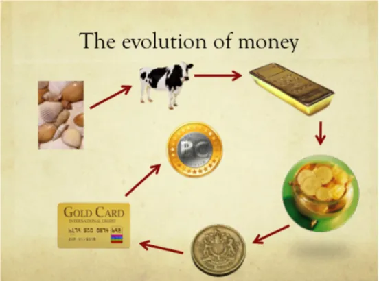
Figure 2.1: Evolution of money (Source: Steemit 2017)

Figure 2.1 in [71]. The evolution of money from 9000 BC until 2018 is described (Steemit 2017)

(16)

2.2 Cryptography

In the ancient time during war periods, generals were trying to communicate with each other secretly with messages in a way that no one else except them could be able to understand the content of it. One person that frequently used that technique was Julius Caesar who was replacing the order of letters [15]. Only those who knew Caesar’s order of change could decode the message. Defining two important features, called encryption and decryption will help us to understand what cryptography is.

2.2.1 Encryption - Decryption

In telecommunications, the message that is clear and easy to read without any unusual activ-ity is called cleartext or plaintext [13]. However, encryption [13] is the method of encoding cleartext in such a way that only empowered persons can understand it’s content. An en-cryption algorithm called cipher, transforms the plaintext into a very hard, almost unreadable raving text called ciphertext. Ciphertext can be well read when is decrypted. Decryption is the procedure of converting the ciphertext to it’s initial cleartext [13].

Figure 2.2: Encryption and decryption (Source: Kalaitzis 2018)

(17)

2.2.2 What is Cryptography?

Cryptography has been used for thousands of years and derives from the Greek words kryptos (hidden, secret) and graphein (to write) [21]. Essentially is the method of sending a message in a concealed way to prevent other parties from reading it. The transmission of information becomes secure with the help of cryptography. Modern cryptography has become an indis-pensable science that combines mathematical theory and computer science to encrypt and decrypt the data. Cryptography is useful for user authentication and in protecting the data from thieves.

While it’s very serviceable, it’s also extremely frangible from people who want to unlock the content of encrypted messages. Cryptanalysis is the science of breaking and prevailing over cryptographic methods using mathematical techniques [21]. Those who use cryptanalysis techniques are called cryptanalyst and are the attackers of cryptography. Cryptology incor-porates the research of both cryptography and cryptanalysis. It derives from the Greek words "kryptos" and "logos" meaning hidden and word respectively. Those who are professionals in this field are called cryptologists.

2.2.3 What is Cryptocurrency?

Cryptocurrency is a digital currency, based on principles of cryptography and on a peer-to-peer network [58]. Virtuality and decentralization make cryptocurrencies autonomous by any central authority like a government or bank and the production, movement and transaction are made entirely in electronic form between the participants. Due to its electronic nature, crypto-currencies are extremely easy to use in different countries without having any restrictions.

Transaction fees are extremely low compared to the high fees that banks impose. Cryptocur-rencies use cryptography for two major purposes. Firstly, to make sure that transactions are secured and secondly having control-govern of the monetary issuance. In 2009, BTC was the first cryptcurrency been made and today there are more than 1500 existing cryptocurren-cies over the Internet. Cryptocurrencryptocurren-cies are also relying on blockchain technology for their functionality and safety.

2.3 What is Blockchain?

Imagine a transaction between three parties A, B, C. Party A is buying a book for 100 $ from party B and party B is buying a sofa for 500 $ from party C. To avoid frauds and make sure that all money has transferred correctly from one party to another, we need someone to keep track of these transactions. On a centralized system, this role is usually assigned to eligible institutions e.g banks which keep track of the details of each transaction on a record called ledger [74]. This procedure takes time to fulfil and undergo with superfluous transactions fees.

(18)

Figure 2.3: Centralized system (Source: Cryptocompare 2018)

Figure 2.3 [17], describes the centralized system and it’s disadvantages.

On the other hand in cryptocurrencies, we are moving from a centralized to a decentralized system. Now instead of only one (bank) having control of the ledger, thousands of hundreds of computers have access to it, verifying each transaction every few minutes. This decentralized public ledger that includes all the cryptocurrency transactions is called blockchain [57]. The blockchain is trustworthy, since the whole community that uses it verifies the same transaction. All the transaction are stored there from the beginning until the present day.

Figure 2.4: Decentralized system (Source: Cryptocompare 2018)

Figure 2.4 [17], describes the advantages of a decentralized system that does not rely on a third party e.g a bank.

(19)

Chapter 3 Bitcoin - Monero

3.1 Bitcoin

3.1.1 What is Bitcoin?

Bitcoin [57] is a digital currency and is probably one of the biggest discoveries in the financial system of the 21st century. It’s production, storage, movement and all transactions with it, is made exclusively in electronic form between the participants of BTC network. No country, government or bank produces or controls BTC.

Users of BTC net interact with each other utilizing a decentralized peer-to-peer network through the internet [3]. This technology is easily approachable and it can run on various electronic devices such as computers and smart-phones. BTC is an open-source digital ex-change and to avoid hacking and achieve safety, it uses cryptographic methods and digital signatures. Anyone can make transactions of BTC and cash but only in specific kiosks and not in the banks. Owners of BTC possess keys, one private and one public which enables them to demonstrate proprietorship of dealings in the BTC network [3]. Ownership of the keys is the only precondition to have the entire control of BTC and they are usually kept in digital wallets on computers.

3.1.2 History of Bitcoin

The idea of distributed cryptocurrency was proposed in 1998 by Wei Dai [18] in the Cypher-punks activist group. After ten years in 2008 and getting inspired from the collapse of Lehman Brothers, an innovative scientific article came up entitled " Bitcoin: A Peer-to-Peer Electronic Cash System " [57]. In 2009, BTC made its first operational appearance with the release of the first open source client and the creation of the corresponding BTC.

The author of the publication and creator of the software remained anonymous using the pseudonym Satoshi Nakamoto [57]. His true identity, even if it is a person or a group, re-mains a mystery to this day. What we know is that Satoshi Nakamoto has been present for a long time on various BTC forums by answering questions. Then in the spring of 2012, he

(20)

disappeared from the Internet. Nakamoto owns a million BTC, which until July 2018 corres-ponds to 8.000.000.000 $.

From 2009 until early 2010, BTC had no value at all. In April 2010, the first transactions in the financial markets began with the value of each BTC not exceeding 0.14 $. At that time, the first commercial transaction was made with the new digital currency. On May 18, 2010, developer Laszlo Hanyecs from Florida made a publication offering 10,000 BTC to anyone who could buy him two pizzas. Four days later on May 22, Jeremy Sturdivant nicknamed "Jarcos" on the forum, accepted the transaction and Laszlo received the two pizza from Papa John’s store.

Figure 3.1: Bitcoin price (Source: Kalaitzis, data retrieved https://www.cryptocompare.com/)

Figure 3.1, shows the BTC price from 2011- 2018.

Looking at the graph, BTC has displayed great changes in its price. For instance in April 2013, there was a 70% drop in its price or 160 $ in one night from 233 $ to 67 $ [7]. Many people believe that this happened due to the outage of Mt.Gox, which is a very popular exchange for making transactions with BTC. Between April and September of 2013, the price of BTC was around 120 $. Then from October until the November of 2013, the price of BTC raised to 1240 $, due to the fact that a big company from China called Baidu started to receive payments with BTC [59]. In December of the same year, the Chinese government banned the use of BTC to all institutions of the country [66] and as a result the price dropped to 800 $. After this bubble, BTC started again to rise but in February 2014 the price fell from 860 $ to 440 $. This occurred because Mt.Gox was hacked, where thieves stole 750,000 BTC [35] from the owners of this platform which today corresponds to 3.000.000.000 $. That incident made a

(21)

big damage to BTC legitimacy and lasted until the late of 2016.

In the early months of 2017, the price started to grow exponentially and in December of the same year climbed to 19.500 $. This was the highest price of all time since BTC was created but in the upcoming of the new year the bubble break and currently, the price has dropped approximately to 7.000 $. This drop can be explained by different facts. Firstly, many companies like Facebook, Google, Twitter has stopped advertising cryptocurrencies [41], [9], [16]. Moreover, South Korea was threatening to close all it’s cryptocurrency exchanges due to abnormal speculation [33]. The most important reasoin is that 80% of the total BTC has been mined already [27].

3.1.3 Transactions with Bitcoin

The way to store and make purchases with BTC is with a BTC wallet [3]. The wallet can be located either as a program on our computer or hosted on a website, e.g. a Bitcoin Exchange. Each BTC wallet has a unique address which make BTC transfer anonymously. All BTC are sharing in the wallets of parties who participate in the coinage network. This is the reason the system is peer-to-peer, because it depends on peers and not on a bank. When a transaction occurs, the system confirms the addresses of two different wallets, the buyer’s and the seller’s.

Afterwards, some mathematical calculations are made to confirm the validity of the transac-tion. These calculations are necessary for cryptographic algorithms that protect the peer-to-peer system, which is based on mathematical security protocols. Once the calculations finish, every valid transaction is recorded. The block log data are added to a public log file called blockchain.

3.1.4 Production of Bitcoin

In a completely digital currency without any central authority who prevents a hacker from creating one billion or one trillion of BTC with a few clicks on the computer? Fortunately, the creator of BTC has predicted about it in a way that is genius.

The key to running BTC is the blocks we mentioned above and the confirmation of transac-tions. To confirm each transaction as valid, the block describing it must be "solved" that is, the data included in it with the proper process must return a mathematical result of a partic-ular form that proves the authenticity of the block. This is important for the security of the entire system so that there can be no forgery blocks for transactions that have not been made or weren’t able to trade with Bitcoin that did not originate from a valid transaction. In fact, the system is designed so that each new block confirms the authenticity of the previous block as a chain (of which the whole log file is called a blockchain). However, as the chain grows the process of solving the blocks becomes more complex and with the absence of a central server to make the calculations, the workload is shared among users who participate anonymously.

(22)

The process of confirming transactions through the solution of each block is called mining and the people involved are called miners [61]. This process takes 10 minutes on average and their reward lending the processing power of their computer is to get new BTC with each block they resolve, as well as commissions resulting from transactions [3]. In fact, the complete confirmation of a transaction gives the miner a reward for a number of BTC gathered.

When BTC first appeared, BTC miners (block solvers) were very few and their computers were of normal speed. At that time, it was possible for someone to run the program for BTC mining on his computer and gather in a relatively short space of hundreds of BTC. One BTC can be divided into 100 million units called "satoshis" [12]. The more miners are involved with powerful equipment, the more difficult the process will be. BTC itself is designed to make the process difficult.

Furthermore, in order not to increase uncontrollably BTC and thus remain limited, the fee for solving the block is planned every four years to drop in half. Up to 2012 was 50 BTC. In 2016 was 12.5 and in 2020 will be 6.25 and so on. Based on this model, the year 2140 will produce the latest BTC and the total number of BTC available will be 21 million [57]. No new BTC will be produced after this number and mining fees (to continue operating) will come exclusively from commissions.

3.2 Monero

3.2.1 What is Monero?

Monero (XMR) [34], is a cryptocurrency intending to be an exchangeable and inexpensive digital exchange tool. It’s production, storage and all transactions with it are made exclusively in electronic form between the community of XMR network. It is not produced or controlled by any particular bank or government and it’s completely private.

It is an open-source proof-of-work (PoW) [76] cryptocurrency, standing out for two reasons: it’s untraceable and it has an inherently greater degree of privacy than any various cryptocur-rencies like BTC which have a transparent blockchain. Having a transparent blockchain gives the opportunity to everyone to trace the location of the transactions and probably linked it with the owner of them, whereas in XMR situation this can’t happen.

It can be run to all major operating systems and is accessible from everyone. To record the transactions, XMR uses a public ledger like BTC but its functionality is not based on BTC code. Contrasting with BTC, XMR is based on the CryptoNote protocol [76] which uses strong encrypting techniques to conceal the parties addresses as well as the amount of money transacted. Today is one of the top 13 out of 100 cryptocurrencies regarding its market capit-alization (number of shares * current market price of one share).

(23)

Figure 3.2: Top 13 cryptocurrencies by market capitalization (Source: Kalaitzis, data retrieved https://www.cryptocompare.com/)

Figure 3.2 shows the top 13 cryptocurrencies with respect to market capitalization. As we can see BTC is the biggest regarding the market capitalization followed by ETH, XRP and BCH, with XMR standing on the 12 place.

3.2.2 History of Monero

The author and creator of CryptoNote protocol that XMR is based on, was inaugurated in Oc-tober 2013 by the pseudonymous name Nicolas van Saberhagen [76]. Monero has it’s roots from another cryptocurrency named Bytecoin [34], which was created by an anonymous per-son around 2014. Shortly after the launch of Bytecoin, many members of the cryptocurrency community were concerned about the lack of credibility and quality of code that it had. One member of Bitcointalk "thankful for today", discovered the limitations of Bytecoin and to-gether with other members of the community, decided to fork it and improved it with stronger code. Eventually, the 18th of April 2014, Monero was launched with the name BitMonero but after some days the team decided to shorten it to Monero.

XMR headers are seven developers, where five of them are anonymous with the pseudonym-ous: Smooth, NoodleDoodle, TacoTime, Eizh, Othe and two that we know their identity which are Riccardo Spagni as "FluffyPony" and David Latapie [34]. Today the value of Monero is 230 $ with market capitalization of 3,316,809,528 $.

(24)

Figure 3.3: Monero price (Source: Kalaitzis, data retrieved https://www.cryptocompare.com/)

Figure 3.3, shows the XMR price from February 2015- July 2018.

3.2.3 Features of Monero

XMR has unique features that make it preferable over the other hundreds of cryptocurrencies. Below we will explain the reasons for choosing XMR over the others.

To begin with, XMR is based on the CryptoNote protocol using CryptoNote encryption. This type of encryption utilizes ring signatures to hide the data of each transaction, which guar-antees that every transaction is kept private and publicly invisible on the blockchain. XMR team has made an improvement on CryptoNote technology providing with a non-transparent system called view key. View key can convert the system transactions completely transparent if the user desires it and only with a private key can see the history of its own transactions referring to the account.

XMR is completely fungible, meaning that it can be interchangeable to different cryptocurren-cies. Since XMR is completely private, no one can identify the transaction trail of it. If people knew that the cryptocurrency that they hold was used in illegal transactions then it wouldn’t be preferred and it would lose its value. The term "clean" or "black" money can’t be attributed to Monero so that’s why is fungible.

(25)

3.2.4 Production - Transactions with Monero

XMR is an open-source proof-of-work (PoW) cryptocurrency. CryptoNote encryption makes the procedure of mining (production) very easy because it allows miners to do mining only by using normal and ordinary CPUs. Everyone can do mining efficiently from their computer without cooperating or paying a lot of money in powerful systems as in BTC case. Moreover, the transactions taken place in XMR block system are extremely fast, requiring simply two minutes [34] in contrast with BTC that needs 10 minutes to complete a transaction. The way to send, store and make purchases with it, is through an XMR wallet. This wallet is private, secure and digital which utilizes the XMR blockchain to protect itself. Now let’s see how the transactions take place in XMR network.

Imagine two parties A and B where party A sends XMR to party B. Then this transaction will be included in an XMR "block" by the XMR network. A block is a file of a series of transactions that have been announced in the XMR network. After that, it takes two minutes for the miners to confirm the first blocks. After 10 "confirmations" which is the successful mining, the transaction is regarded entirely verified. After this procedure, your wallet will notify you, usually after 4-10 minutes about the transaction.

XMR total coin supply is a little different than BTC. On May 31, 2022, the total number of XMR coin will reach 18.3 million. From that point on, rising of supply will be limited to a rate of 0.3 XMR per minute or 157788 XMR per year. This is a constant amount and it will be decreased every year but it will never reach 0 [34]. This is meant to provide motivation to ensure the Blockchain even after the total number of XMR coins will be distributed. In 2140, XMR and BTC will both have nearly 21 million coins.

3.2.5 XMR Major Anonymity Techniques

Monero network uses 4 different cryptographic techniques to establish privacy for its users: ring signatures, stealth addresses, RCT (Ring Confidential Transactions) and Kovri. Each of those techniques has a specific role for the transactions privacy. Those techniques makes Monero standing out from other cryptocurrencies.

• Ring Signatures

Ring signatures are essentially an advanced, mandatory system for transaction mixing ad-dresses which conceals sender’s information and ensures its privacy [34]. In this technique the transaction is been signed by a group of users, making it infeasible to track who was the original sender. With the use of digital signatures, the real signer is hiding among numerous ring members, making it easier to validate a transaction and being untraceable.

(26)

• Stealth Address

A stealth address, known as a one-time public key, prevents external viewers from identifying the receiver address of a transaction [34]. A 3rd party can audit that address to validate the transaction occurred. The sender has to generate a public view key for the recipient and send XMR through this key. After the recipient is using a private view key to scan the whole blockchain to find the funds that have been sent to him [82]. Once detected, a private key is generated correlative with senders public key and the recipient can use those funds. The XMR address is composed by the one-time public key and the private key. Even though the transaction is registered on the blockchain, only the parties that took part in the transactions, the receiver and the sender can specify the location of the transaction [34].

• Ring Confidential Transactions (RCT)

Ring Confidential Transactions (RCT), was activated on January 9, 2016 and conceals the amount of XMR that is being transferred [60]. Only parties A and B will know the real amount of money that is transferred whereas the miners will only have enough information to validate the transaction. Then the transaction is considered as authentic and the user doesn’t losses his privacy.

• Kovri

The main concept of everything that XMR is developing is focused on privacy and anonymity. Nowadays XMR has made a great step to provide complete anonymity and privacy with the use of Kovri. Kovri is a free anonymity software, based on I2P’s open specification, allowing users to make entirely private transactions [34]. Kovri can be used by everyone around the world who needs anonymity in his job, regardless of whether the user is familiar with crypto-currencies or not. By using encryption and routing techniques called garlic, Kovri manages to produce an anonymous overlay network through the internet that conceals both the IP address which is the address of the internet that users have and the geographical position of them [34].

(27)

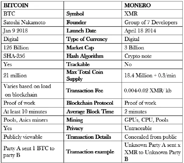
3.3 Bitcoin vs Monero

After explaining each cryptocurrency, it’s time to compare [78] them and see their differences. After the comparison, everyone can have a general idea on which cryptocurrency is better to invest.

Figure 3.4: Bitcoin - Monero comparison (Source: Kalaitzis 2018)

Figure 3.4, shows the differences of BTC and XMR.

As we can see, XMR has some advantages over BTC such as the average blocking time where it needs only two minutes in contrast with BTC that needs at least ten minutes. XMR is completely private and untraceable whereas in BTC case, someone can trace the location of the user through the IP address. Also in XMR, the mining can be done easily with GPUs, CPU. On the other hand, BTC market capitalization and price is way bigger than XMR.

(28)

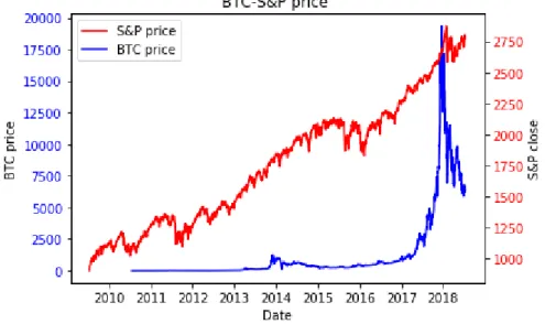
Figure 3.5: BTC - XMR price (Source: Kalaitzis, data retrieved from ht-tps://finance.yahoo.com/)

Figure 3.5, compares the prices of Bitcoin and Monero .

As we can notice, BTC and XMR prices are moving quite together both when the prices rises and when prices falls. After, we will see how much those cryptocurrencies are correlated with each other.

Figure 3.6: Bitcoin - Monero yearly close price (Source: Kalaitzis, data retrieved from ht-tps://finance.yahoo.com/)

Figure 3.6, compares the yearly closing prices of Bitcoin and Monero .

We can clearly see that BTC is more expensive than XMR as it has been the first cryptocur-rency created from 2009. The most profitable year for both of them was 2017, when they had their highest prices.

(29)

Chapter 4 VIX

4.1 Volatility

4.1.1 What is Volatility

Volatility plays a major role in mathematics and especially in finance and when it drops or increases it affects the markets. But what does the term volatility exactly mean?

Practically, volatility(σ ) is the tendency of something to change considerably and in finance is referred as the rate at which the price of a security alters over a given period of time. Ad-ditionally, it is mentioned as the standard deviation and is computed as a percentage, derived from a mathematical formula. When a security has a relevant steady price, then it has low volatility and when a security is susceptible to rapidly price movements, it has high volatility.

Volatility helps us to calculate the risk of a financial instrument and to evaluate the fluctuations that take place in a small period of time. Volatility is driven by various factors both econom-ical (high taxes) and natural (earthquakes) etc. When volatility is low, indices like VIX and S&P500 have better returns.

4.2 Types of Volatility

4.2.1 Realized Volatility - Historical Volatility

Realized volatility was presented by Bandorff - Nielsen and Sheppard [5] and it is obtained from the realized variance RV =

n

∑

i=1 r_i2, where r_i= log( Pi Pi−1 ), i = 1, 2, .., n − 1, n

is the intraday returns of the asset. To calculate the price variability of asset prices, it is man-datory to use practical data. Assuming that Pt, is the asset price of an asset at time t, the

(30)

annual-ized realannual-ized volatility on the interval [t1,t2] based on n + 1 daily observances P0, P1..., Pn−1, Pn, is given by RV_ol = s 252 n− 1 n

∑

i=1 r2_i, where n

∑

i=1 r_i2: Realized variance (RV)

252: The number of trading days in a year. We are dividing by n − 1, as we are calculating the standard deviation from a sample.

Historical volatility is the realized volatility of the underlying asset over a preceding time looking at previous fluctuations in price [62]. It is defined by measuring the standard deviation of the underlying asset returns from the mean during that time and is based on alterations in the stock’s price. For a contract with T days to maturity at time t, the historical volatility is computed by using the daily return of the period, going back T days from time t and it can be calculated in different periods, from a week until a year.

One important feature of historical volatility is that it doesn’t show into which direction the stock will move. A low historical volatility indicates that the stock hasn’t been moving much over a period of time and a high historical volatility means that prices are moving up and down faster than usual and it is a sign that something will change. The formula of the historical volatility [25] is determined as σn= s 252 n− 1 n

∑

i=1 (ri−er) 2_, where er= 1 n n

∑

i=1 r_i.

The_eris the mean of the daily returns and the historical volatility is the yearly sample standard deviation if the returns come from the same distribution. That’s also the reason why we are dividing by n − 1.

We can see that

n

∑

i=1 (ri−er) 2₌ n

∑

i=1 r_i2− n_er2,

(31)

and therefore

σ_n2= RV_ol2−252ner n− 1.

If_eris nearly close to zero, then the realized and the historical volatility are roughly equal and they are called realized variance and historical variance. Usually the realized and the historical variance are used to forecast future volatility.

Figure 4.1: BTC volatility (Source: Kalaitzis, data retrieved from https://finance.yahoo.com/)

Figure 4.1, shows the volatility of BTC from 2011 - 2018 .

Figure 4.2: XMR volatility (Source: Kalaitzis, data retrieved from https://finance.yahoo.com/)

(32)

Figure 4.3: BTC - XMR volatility (Source: Kalaitzis, data retrieved from ht-tps://finance.yahoo.com/)

Figure 4.3, compares the volatility of Bitcoin and Monero.

4.2.2 The Implied Volatility

Implied volatility, is the volatility of a financial instrument which when is computed by option pricing models, for example, the Black - Scholes model, will give us a notional value to the present price of the option [51]. As we mentioned, it is only an approximation and there is no commitment that an option price will follow the predicted way. The difference between the historical volatility and implied volatility is that historical volatility shows us the movement of stock price during past terms, whereas implied volatility shows the movement of stock price that may have in the future [39].

Implied volatility can be calculated from the Black - Scholes (BS) model [8]. BS model is a mathematical model that helps us to estimate the price of European call and put options. The BS formula is based on the geometric Brownian motion assumption for the underlying asset price which has constant volatility. Theoretically, the volatility in Black - Scholes is a constant but in practice, we must use alternative volatility with alternative strike prices K to be equal with the market prices. Unfortunately, the value is not known and we must calculate it. Implied volatility is derived from the Black - Scholes formula and is a great principle of how the value of options are resolved.

Assume a non-negative price process Stand a stock that pays no dividend. A call option has a pay-off (ST− K)+ where T is the maturity day, the underlying asset in maturity ST and K is the strike price. The option price is a function C of the volatility of the stock’s price (the higher the volatility the higher the premium on the option) and the other variables K, T, today’s date

(33)

t, the underlying asset St.

The risk-free interest rate is a constant r and

x= log( K S_ter(T −t)) the log-moneyness of an option.

Assuming frictionless markets (markets without restraints and transaction costs), Black and Scholes denoted that if Stfollows Wt: Wiener process with respect to a risk-neutral probability measure. [51] (definition of Brownian motion is given in the next chapter)

dS_t = µStdt+ σ StdWt (4.1) where µ is the drift rate of St and the no-arbitrage (a state in which the assets are priced properly and the person’s profits can’t outperform market profits) price is

C= CBC(σ ), (4.2)

Then the price formula [8] is:

CBC(σ ) = CBC(St,t, K, T, σ ) = N(d1)St− N(d2)Ke−r(T −t) (4.3) where d₁=ln( Ster(T −t) K ) σ √ T− t + σ √ T− t 2 (4.4) and d2= d1− σ √ T− t (4.5)

Additionally, if we know C(K, T ), then the implied volatility for strike price and maturity date K, T respectively is determined as I(K, T ) solving the C(K, T ) = CBS(K, T, I(K, T )) where the solution is monadic. It is monadic, because CBS is strictly increasing in σ and as σ −→ 0 (respectively (∞)), CBC(σ ) approximates the lower (respectively upper) no-arbitrage bounds on a call. [51]

(34)

4.3 CBOE Volatility Index (VIX)

In 1973, when the stock options transactions started, one of the senior futures and options exchanges, the Chicago Board of Trade (CBOT), founded an another exchange called the Chicago Board Options Exchange (CBOE) [26]. CBOE is an exchange focusing on trading options contracts, comprising interest rate, index, foreign currency and stock options. Offering 22 stock indices and options of more than 2000 companies, CBOE is the biggest U.S options exchange and the 2nd in the world behind the Korea Stock Exchange (KSE). At 2014, it’s yearly exchanging volume was 1.27 billion contracts.

In 1993, Professor Robert Whaley presented a paper "Derivatives on Market Volatility: Hedging Tools Long Overdue" [79] introducing the VIX index for the CBOE. VIX index usually men-tioned as the "fear index" it was initially created to compute the market’s anticipation of 30-day implied volatility by at-the-money S&P 100 Index (OEX Index) option prices [26]. In 2003, VIX was improved to measure the implied volatility of the S&P 500 Index (SPX). S&P 500 is issued by 500 large companies and is one of the biggest U.S stock market index and is the main standard for U.S stock market volatility.

VIX index informs us of the market view on volatility in the near future and every 15 seconds throughout the trading hours it is calculated to measure volatility. A characteristic of the VIX index is that includes historical prices of more than 20 years ago. This is a valuable help for the investors as they can see the behaviour of the option prices back in time in response to different market circumstances. It is great of importance to become aware of that VIX index is a forward-looking measure of volatility and is computed from both call and put options. It is indicated by the present prices of S&P 500 index options and stands for anticipated future market volatility over the next 30 days.

Figure 4.4: S&P500 price from 2006 - 2018 (Source: Kalaitzis, data retrieved from Yahoo Finance, https://finance.yahoo.com/)

(35)

4.4 Evolution - Interpretation of VIX

In 1993, the VIX index was initially created to calculate the market’s anticipation of 30-day implied volatility by at-the-money S&P 100 Index (OEX Index) option prices [26]. After some years VIX was improved and CBOE computed other volatility indexes. In 2001, CBOE computed the NASDAQ 100 index as the underlying volatility index (VXN) [81]. In 2003, three new indexes came up: The S&P 500 Index, measuring the implied volatility of the S&P 500 Index options (SPX), the CBOE DJIA volatility index (VXD) and CBOE Russell 2000 volatility index (RVX) [26]. After one year in 2004, CBOE computed another two: the VIX futures which stands for the volatility index futures and S&P 500 3-month volatility Index (VXV).

The VIX index options started to trade in the CBOE in 2006 and in 2008 CBOE was the first to introduce and evaluate the expected volatility of different currencies and commodities [26]. Today, CBOE has presented new volatility indexes based on big companies stocks such as VIX on Amazon (VXAZN), Apple (VXAPL), Google (VXGOG), IBM (VXIBM) etc. VIX and S&P 500 are both computed indexes with the difference that the VIX is not derived from stock prices. By utilizing the options prices of the S&P 500, VIX evaluates how volatile those options will be between the option’s present-day and the maturity date. It is important to mention that VIX is just a prediction of market volatility and not the real volatility of the future. It is a general expectation based on the options premiums that people are eager to pay.

The method of calculating the VIX index has changed several times in the past. In the early 1990s, volatility resulted from the Black-Scholes pricing model given the one-option (only for at-the-money options). There were many flaws in the initial calculation of VIX as it contained only 100 shares. It did not adequately represent the stock market and the variability calculated by the Black-Scholes model is not accurate as the model itself is considered unreliable in several cases.

The new VIX calculation followed a more sophisticated approach that does not rely on known models, calculating volatility from a weighted average of a wide range of strike prices both in-the-money and out-of-the-money options (call / puts) of the S&P 500 index. A few years ago, derivatives were included in the volatility-fear index. In fact, simply switching from the S&P 100 to S&P 500, the VIX index displayed a greater correlation with actual market volat-ility. Using a wide range of strike prices rather than just at-the-money options, the volatility calculation is more accurate taking into account the volatility smile phenomenon.

(36)

Figure 4.5: VIX price from 2006 - 2018 (Source: Kalaitzis, data retrieved from Yahoo Finance, https://finance.yahoo.com/)

Figure 4.5, shows the VIX price from 2006 - 2018.

The fear index is broadly supposed to comply with the below interpretations:

• 5 - 20 = low anxiety

• 20 - 30 = moderate anxiety

• 30 - 45 = high anxiety

• 45 - 60 = panic

• 65+= extreme panic

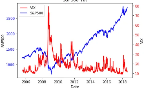
VIX is charted on a scale from 1-100 and is given by percentage, symbolizing how much the S&P 500 index option (SPX) will fluctuate over the next year at 68% confidence level. For instance, if the VIX is 20, that means that there is 68% probability of trading within a range 20 higher or lower than it’s present volume over the next 12 months. If we want to compute for one month, then we have to divide the VIX level by the square root of 12, which represents the months of a year. VIX and S&P 500 usually move opposite to each other and the rate is usually 3-4 times. For example, if the S&P 500 rises 1% then VIX suffers a loss of 3-4%.

(37)

Figure 4.6: S&P500 and VIX (Source: Kalaitzis, data retrieved from Yahoo Finance, ht-tps://finance.yahoo.com/)

Figure 4.6, compares the prices of S&P500 and VIX.

The VIX index is used by option traders to calculate option premiums and also by S&P 500 traders to determine the expected fluctuation of S&P 500 and futures markets. While crit-ics of the method claim that its usefulness are overvalued, the index is considered to be the most important volatility index of options in the wider market. Prior to the VIX introduc-tion, investors considered whether the market was unstable or not based on their experience. VIX literally quantified the concept of volatility, allowing investors and traders to use it as a stability indicator, trade it or use it for hedging.

In the insurance field, premiums can be seen as a form of risk and depend on the value of risk, the premiums are changing either up when the risk is great or down when the risk is low. This happens exactly in the case of VIX. When the option premiums rise, then the VIX also rises and vice versa. The VIX is set by thousands of traders who make billions of transactions and those who buy and sell fluctuate the price of the options. More buyers raises the value of premiums and more sellers lower the value of it. After the CBOE combines the price of the options in the S&P 500 index coming out with a number named VIX. This number displays if investors are paying more or less for the options premiums of the S&P 500 index.

(38)

4.4.1 Comparison BTC - XMR - S&P500 - VIX

From Yahoo Finance, we obtained the daily data for the S&P500 and the VIX. Below we will see graphs of BTC price and volatility with respect to S&P500 and the VIX.

Figure 4.7: Bitcoin - S&P500 price (Source: Kalaitzis, data retrieved from Yahoo Finance, https://finance.yahoo.com/)

Figure 4.7, compares the prices of Bitcoin and S&P500.

Figure 4.8: Bitcoin volatility - S&P500 price (Source: Kalaitzis, data retrieved from Yahoo Finance, https://finance.yahoo.com/)

(39)

Figure 4.9: Bitcoin price - VIX (Source: Kalaitzis, data retrieved from Yahoo Finance, ht-tps://finance.yahoo.com/)

Figure 4.9, compares the price of Bitcoin with the VIX index.

Figure 4.10: Bitcoin volatility - VIX (Source: Kalaitzis, data retrieved from Yahoo Finance, https://finance.yahoo.com/)

(40)

Now let’s have a look on the relation between Monero(XMR) and the S&P 500, VIX

Figure 4.11: XMR - S&P500 price (Source: Kalaitzis, data retrieved from Yahoo Finance, https://finance.yahoo.com/)

Figure 4.11, compares the price of Monero with the S&P500 price.

Figure 4.12: XMR volatility - S&P500 price (Source: Kalaitzis, data retrieved from Yahoo Finance, https://finance.yahoo.com/)

(41)

Figure 4.13: XMR price - VIX (Source: Kalaitzis, data retrieved from Yahoo Finance, ht-tps://finance.yahoo.com/)

Figure 4.13, compares the price of Monero with the VIX index.

Figure 4.14: XMR volatility - VIX (Source: Kalaitzis, data retrieved from Yahoo Finance, https://finance.yahoo.com/)

(42)

4.4.2 The VIX Calculation - Derivation

The VIX is computed using the following formula [26]:

σ2= 2 T

∑

_i ∆Ki K_i2 e RT_Q(K i) − 1 T[ F K0 − 1] (4.6) where σ =V IX₁₀₀

T : The time to maturity

F : Forward index level desired from index option prices

K₀: First strike below the forward index level, F.

K_i : Strike price of the ith out-of-the-money option. A call, if Ki> K0 and a put if Ki< K0, both put and call if Ki= K0.

∆Ki: Interval between strike prices - half the difference between the strike on either side of Ki

∆Ki=

Ki+1− Ki−1 2

(Note : ∆K for the lowest strike is simply the difference between the lowest strike and the next higher strike. Likewise, ∆K for the highest strike is the difference between the highest strike and the next lower strike.)

R: Risk-free interest rate to expiration.

Q(Ki) : The midpoint of the bid-ask spread for each option with strike Ki.

Now we will give the derivation of the VIX formula and it is the following. Let’s hypothesize that the price of the stock follows the differential equation

ds

S = (r − q)dt + σ dW (4.7)

where

r: Risk free rate

(43)

σ : Stochastic volatility

W : Wiener process with respect to a risk-neutral probability measure.

From the Ito’s lemma

d ln S = (r − q −σ 2

2 )dt + σ dW (4.8)

Then by subtracting the two equations (4.7) - (4.8) we get

ds S − d ln S = (r − q)dt + σ dW − (r − q − σ2 2 )dt + σ dW = σ2 2 dt ds S − d ln S = σ2 2 dt (4.9)

If we integrate from time 0 to time T , we obtain

Z T 0 σ2 2 dt= Z T 0 ds S − Z T 0 d ln S ⇒ 1 2σ 2_T ₌Z T 0 ds S − (ln ST − ln S0) where S0: the underlying asset in time 0

⇒ 1 2σ 2_T ₌Z T 0 ds S − ln( S_T S0 )

The realized average variance rate is the square of the volatility ¯V and so we have

1 2V T¯ = Z T 0 ds S − ln( S_T S0 ) ¯ V = 2 T Z T 0 ds S − 2 T ln( S_T S₀) (4.10)

Then by taking the expectations of the previous equation

b E[ ¯V] = 2 TE(b Z T 0 ds S ) − 2 TEb(ln S_T S₀), (4.11)

(44)

b E( Z T 0 ds S) = bE[ Z T 0 (r − q)dt] + bE( Z T 0 σ dz) ⇒E(b Z T 0 ds S ) = (r − q)T. (4.12)

Putting the equation (4.12) into the equation (4.11) we have

b E[ ¯V] = 2 T(r − q)T − 2 TE[ln(b S_T S₀)].

We already know that

S_T = S0exp(X ) and

X = [r − q −σ 2

2 T+ σ z(T )] is normal with expectation and variance respectively

b E[X ] = (r − q −σ 2 2 )T d Var[X ] = σ2T. Then b E[ST] = S0exp( bE[X ] + d Var[X ] 2 ) = S0e (r−q)T_, Consequently b E[ ¯V] = 2 T ln( F₀ S₀) − 2 TE[ln(b S_T S₀)], (4.13) where F₀= bE[ST]

is the forward price of the asset for a contract maturing at time T .

(45)

Z S?

0 1

K2max(K − ST, 0)dK. S?Let us denote a value of S by S?.

If • S?< ST: Z S? 0 1 K2max(K − ST, 0)dK = 0. • S?_{> S} T: Z S? 0 1 K2max(K − ST, 0)dK = Z S? ST 1 K2max(K − ST)dK = (ln K +ST K S? ST ) = ln(S ? ST ) +ST S? − 1. Furthermore we consider Z _∞ S? 1 K2max(ST − K, 0)dK. If • S?_{> S} T: Z ∞ S? 1 K2max(ST− K, 0)dK = 0. If • S?< ST: Z ∞ S? 1 K2max(ST − K, 0)dK = Z ST S? 1 K2(ST − K)dK = (−ST K − ln K) ST S? = −1 − ln ST+ S_T S? + ln S ? = ln(S ? S_T) + ST S? − 1,

(46)

From these results we can get Z S? 0 1 K2max(K − ST, 0)dK + Z _∞ S? 1 K2max(ST− K, 0)dK = ln( S? S_T) + S_T S? − 1 for all values of S?such that

ln(S ? ST ) =ST S? − 1 − Z S? 0 1 K2max(K − ST, 0)dK − Z ∞ S? 1 K2max(ST − K, 0)dK. (4.14) Taking expectations with respect to the risk-neutral probability measure in equation(4.14)

b E[ln(S ? S_T)] = bE[ln( ST S?) − 1] − bE[ Z S? 0 1 K2max(K − ST, 0)dK] − bE Z ∞ S? 1 K2max(ST− K, 0)dK Notice that b E[max(K − ST, 0)] = eRTp(K), b E[max(ST− K, 0)] = eRTc(K), and F₀= bE(S_T), where

c(K) : Price of the call option

p(K) : Price of the put option

K : Strike price

T : Time to maturity

R: Risk-free interest rate for a maturity of T .

Furthermore b E[ln(S ? S_T)] = F0 S?− 1 − [ Z S? 0 1 K2e RT_{p(K)dK −}Z ∞ S? 1 K2e RT_c(K)dK]. _(4.15) We know that

(47)

ln(ST S₀) = ln ST − ln S0 = ln ST − ln S?+ ln S?− ln S0 = ln(ST S?) + ln( S? S₀).

Again we will take the expectation of the previous equation and we will get

b E[ln(ST S₀)] = bE[ln( S_T S?)] + bE[ln( S? S₀)] = ln(S ? S0 ) + bE[ln(ST S?)]. (4.16)

Now we will combine equations (4.13), (4.15), (4.16)

b E[ ¯V] = 2 T ln( F₀ S₀) − 2 TE[ln(b S_T S₀)] = 2 T ln( F0 S₀) − 2 T{ln( S? S₀) + bE[ln( ST S?)]} = 2 T ln( F₀ S₀) − 2 T{ln( S? S₀) − 2 TE[ln(b S_T S?)]} = 2 T ln( F₀ S0 ) − 2 T{ln( S? S0 ) − 2 T F₀ S?− 1 − [ Z S? 0 1 K2e RT_{p(K)dK −}Z ∞ S? 1 K2e RT_c(K)dK]} = 2 T(ln F0− ln S0− ln ? S+ ln S0) − 2 T F₀ S?− 1 − [ Z S? 0 1 K2e RT_{p(K)dK −}Z ∞ S? 1 K2e RT_c(K)dK] = 2 T(ln F0− ln S0) − 2 T{ F0 S?− 1 − [ Z S? 0 1 K2e RT_{p(K)dK −}Z ∞ S? 1 K2e RT_c(K)dK)]} = 2 T ln( F₀ S?) − 2 T( F₀ S?− 1) + 2 T[ Z S? 0 1 K2e RT_{p(K)dK +}Z ∞ S? 1 K2e RT_c(K)dK]. (4.17)

Finally, the equation (4.18), is the expected value of the average variance

b E[ ¯V] = 2 T ln( F₀ S?) − 2 T( F₀ S?− 1) + 2 T[ Z S? 0 1 K2e RT_{p(K)dK +}Z ∞ S? 1 K2e RT_c(K)dK]. _(4.18)

Suppose that we know the prices of the option’s, having Kifor strike prices where K1< K2< .... < K_nand S?equal to the first strike price below F0, the integrals can be approximated by

(48)

Z S? 0 1 K2e RT_{p(K)dK +}Z ∞ S? 1 K2e RT_{c(K)dK ≈}

∑

i ∆Ki K_i2 e rT_Q(K i), (4.19) where

Q(K_i) : The midpoint of the bid-ask spread for each option with strike K_iand

∆Ki=

Ki+1− Ki−1

2 , 2 ≤ i ≤ n − 1.

If we put the equation (4.19) into equation (4.18), we will get

b E[ ¯V] = 2 T ln( F₀ S?) − 2 T( F₀ S?− 1) + 2 T[ n

∑

i=1 ∆Ki K_i2 e rT_Q(K i)] ⇒E[ ¯bV]T = 2 ln( F₀ S?) − 2( F₀ S?− 1) + 2[ n

∑

i=1 ∆Ki K_i2 e rT_Q(K i)] (4.20)

We can expand the ln(F0

S?) in Taylor series as ln(F0 S?) = ( F0 S?− 1) − 1 2( F0 S?− 1) 2₊1 3( F0 S?− 1) 2₋1 4( F0 S?− 1) 2_....

and it can be approximated as

ln(F0 S?) = ( F₀ S?− 1) − 1 2( F₀ S?− 1) 2 . ⇒ ln(F0 S?) − ( F₀ S?− 1) = − 1 2( F₀ S?− 1) 2 _(4.21) Substituting (4.21) in (4.20) we get : ⇒E[ ¯bV]T = 2 ln( F0 S?) − 2[ F0 S?− 1] + 2 T[ n

∑

i=1 ∆Ki K_i2 e rT_Q(K i)] = −(F0 S?− 1) 2 + 2[ n

∑

i=1 ∆Ki K_i2 e rT_Q(K i)]. (4.22)

The final form of the VIX formula is (proof is adapted from [39], [42] )

σ2= −1 T( F K0 − 1)2+2 T[ n

∑

i=1 ∆Ki K_i2e RT_Q(K i)]. (4.23)

(49)

Chapter 5 Correlation

5.1 Time Series

Time series is a group of data points which is usually graphed over time and has applications in statistics, econometrics and in many other domains of applied science [37]. For instance, the temperature of a day in summer at hourly intervals or the price of a stock on ordinal intervals of time, is time series. In other words, a time series can be described as a random variable X , indexed by the time t : Xt;t = 1, 2, 3, ...T .

Time series is used either in an analysis in order to obtain important statistics, either on fore-casting to forecast future outcomes based on formerly outcomes. It is important to mention that the values of time series can be either discrete or continuous.

Figure 5.1: S&P500 volume (Source: Kalaitzis, data retrieved from Yahoo Finance, ht-tps://finance.yahoo.com)

(50)

5.2 Stochastic Processes

Definition 1. A stochastic process is a collection of random variables, X = {X (t) : t ∈ T }, where T is a set of time season’s, with T _{⊂ R. See also [14, Definition 2.2] for a formal} definition of a continuous random variable. [47]

A stochastic process can either be discrete or continuous.

Definition 2. A stochastic process X is called a discrete-time stochastic process, if the in-dex set T consists of consecutive integers, T = {..., −2, −1, 0, 1, 2, ...}, whereas a stochastic process X is called a _{continuous-time stochastic process, if T is an interval of R with T =} [a, b], T = [0, ∞) or T = (−∞, +∞). [49]

Definition 3. The mean function of the stochastic process X is determined as m(t) = E[X (t)], and thevariance function u(t) = V [X (t)]. [1]

Definition 4. A stochastic process is called a second order process, if its second order moment is finite for all t i.e E(X2(t)) < ∞. [67]

Definition 5. The covariance function, C(s,t) is given by

C(s,t) = cov(X (s), (X (t)) = E(X (s)X (t)) − E(X (s))E(X (t)).[54]

Properties of covariance function

(1) C(s,t) = C(t, s), ∀t, s ∈ T

(2) It is non negative definite

n

∑

j=1 n

∑

k=1 ajakC(tj,tk) = E[

∑

ajX(tj)2] ≥ 0 where a1, a2, ...an∈ R and ti∈ T

(3) Applying Schwarz inequality

(51)

Theorem 1. (Cauchy-Schwarz Inequality)

If X and Y are random variables where E[X2] and E[Y2] exists then

(E[XY ])2≤ E[X2]E[Y2]

Proof. [80] Assume

f(t) = E[(X + tY )2] = E[X2] + 2tE[XY ] + t2E[Y2].

Then f is a quadratic polynomial in t with f (t) ≥ 0, ∀t. Consequently by the quadratic formula,

4(E[XY ])2− 4E[X2]E[Y2] ≤ 0. Therefore

(E[XY ])2≤ E[X2]E[Y2]

Before giving the definition of Brownian motion, it is preferably to mention first the definition of normal distribution as Brownian motion is connected with it.

Definition 6. A random variable X, is normally distributed with mean µ and variance σ2if P{X > x} = √ 1 2πσ2 Z ∞ x e−(u − µ) 2 2σ2 du.[72]

Definition 7. A stochastic process {B(t) : t ≥ 0} is called Brownian motion, starting from x_{∈ R if: [56]}

(1) B(0) = x,

(2) for every 0 ≤ t1≤ t2≤ ... ≤ tnthe increments B(tn) − B(tn−1), B(tn−1) − B(tn−2), ..., B(t2) − B(t1) are independent random variables,

(3) ∀t ≥ 0 and ∀h > 0, the increments B(t + h) − B(t) are normally distributed with mean 0 and variance h,

(4) almost surely, the function t → B(t) is continuous.

(52)

5.3 Stationary Process

Broadly speaking, stationarity refers to something that doesn’t change over time. In statistics refers to a random process, where it’s statistical properties doesn’t change over time such as mean or auto-correlation. There are two types of stationarity: strong and weak stationarity.

Definition 8. The time series [Xt,t ∈ Z], is strong stationary, when where given that t1, ....,tk, the joint statistical distribution of(Xt1, ...., Xtk) is the same as the joint statistical distribution of(Xt1+l, ...., Xtk+l) for all k and l. [6]

In simpler words, this definition says that we have strong stationarity when the joint statist-ical distribution depends solely on the difference l, not the time (t1,tk). This means that all moments of all degrees (means, variances, covariances) of the process are the same.

Someone may ask what is so important and all analysts care so much about stationarity? The most important reason is that the majority of the models that we use hypothesize covariance-stationarity. This means that statistics like mean, variance and correlation, are only trustable if the time series is stationary. Unfortunately, the definition of strong stationarity is too strict and difficult to prove it for real-life processes. However, in real life purposes, it is enough to use a weaker definition of stationarity.

Definition 9. The time series [Xt,t ∈ Z], is said to be weak stationary or covariance stationary if

• E[X(t)] = µ, ∀t ∈ Z • E[X2_{(t)] < ∞, ∀t ∈ Z}

• C(s,t) = C(s + h,t + h), ∀t, s, h ∈ Z [6]

To simplify this, a stationary time series [Xt,t ∈ Z] has to have the following characteristics: The mean and the variance have to be constant (not depend on t) and that the C(s,t) only depends on (ts) and not depends on s or t.

Definition 10. Let yt, t= (.., −1, 0, 1, ...) be an n-dimensional stochastic process (n ≥ 1) and let x_t ∈ yt ( with xt= yt, if n=1). The stochastic process xt is a martingale with respect to yt

E(xt|yt−1, yt−2, ..) = xt−1,t = (..., −1, 0, 1, ...), [36] We say that y_tis amartingale, if x_t is a martingale with respect to y_t,∀x_t∈ y_t.

Bitcoin - Monero analysis: Pearson and Spearman correlation coefficients of cryptocurrencies

Bitcoin - Monero analysis: Pearson and Spearman correlation

coefficients of cryptocurrencies

by

Angelos Kalaitzis

MASTER THESIS IN MATHEMATICS/ APPLIED MATHEMATICS

DIVISION OF APPLIED MATHEMATICS

Acknowledgements

Abstract

Contents

List of Figures

List of Tables

List of Abbreviations and Acronyms

Chapter 1

Introduction

Chapter 2

Cryptocurrencies

2.1

The Evolution of Money

2.2

Cryptography

2.2.1

Encryption - Decryption

2.2.2

What is Cryptography?

2.2.3

What is Cryptocurrency?

2.3

What is Blockchain?

Chapter 3

Bitcoin - Monero

3.1

3.1.1

What is Bitcoin?

3.1.2

History of Bitcoin

3.1.3

Transactions with Bitcoin

3.1.4

Production of Bitcoin

3.2

Monero

3.2.1

What is Monero?

3.2.2

History of Monero

3.2.3

Features of Monero

3.2.4

Production - Transactions with Monero

3.2.5

XMR Major Anonymity Techniques

3.3

Bitcoin vs Monero

Chapter 4

VIX

4.1

Volatility

4.1.1

What is Volatility

4.2

Types of Volatility

4.2.1

Realized Volatility - Historical Volatility

∑

∑

∑

∑

∑

∑

∑

4.2.2

The Implied Volatility

4.3

CBOE Volatility Index (VIX)

4.4

Evolution - Interpretation of VIX

4.4.1

Comparison BTC - XMR - S&P500 - VIX