Emission of inhalable particles from studded tyre wear of road pavements : a comparative study

(1)

Mats Gustafsson

Olle Eriksson

Emission of inhalable particles from

studded tyre wear of road pavements

A comparative study

VTI r

apport 867A

|

Emission of inhalable particles fr

om studded tyr

e wear of r

oad pav

www.vti.se/publications

VTI rapport 867A

(2)

(3)

VTI rapport 867A

Emission of inhalable particles from

studded tyre wear of road pavements

A comparative study

Mats Gustafsson

Olle Eriksson

(4)

Omslagsbilder: Mats Gustafsson, VTI Tryck: LiU-Tryck, Linköping 2015

(5)

Abstract

New restrictions on the number of studs on studded tyres were introduced in Sweden and Finland in 2013. Regulations now allows 50 studs per meter rolling circumference. Alternatively, the tyres can be tested in a special wear test, the so-called over-run test, to be approved. This has resulted in studded tyres that follows the rule of the number of studs per rolling circumference meters, but also studded tyres that pass the over-run test, even though they have considerably more spikes are present on the market. The over-run test shall ensure that the tested tyre will not cause more road wear than a tyre with a maximum of 50 studs per meter rolling circumference. Since studded tyres are a major source of inhalable particles (PM10) in road and street environments, it is of interest to investigate the

difference between the various studded tyre types also from particle emission point of view. In the present study, the particle generation from seven studded tyres was tested in the VTI road simulator. The tyres have been tested at 50 km/h in a statistically optimal sequence during the four test days where various order of tyres used each day of testing. Concentrations (mass and number) and size distributions were measured during the experiments, as well as environmental parameters (temperature and humidity). In the statistical analysis of particle data was partly analysed as constants and partly as depending on ambient and tyre-specific parameters.

The results show that the tyre with the most studs (190) generates significantly higher PM10 levels than

other tyres while one of the tyres following the stud number regulations and have 96 studs results in significantly lower formation of inhalable particles than all other tyres tested. Increased number of studs increases PM10, PM2.5 and number concentration significantly, while increasing stud force

significantly increases the concentration of PM10 and PM2.5. Temperatures in the tyre, pavement and

air as well as relative humidity also have an effect on the particle levels. A calculation example was performed where the relationship between the tested highest and lowest emitting tyres was applied in a process based emissions model in which studded tyre wear is included (NORTRIP model). This demonstrated that the effect of variations in the studded tyre wear on both PM10-levels and the number

of limit value exceedances for the current data set used was significant.

Title: Emission of inhalable particles from studded tyre wear of road pavements - a comparative study

Author: Mats Gustafsson (VTI), Olle Eriksson (VTI)

Publisher: Swedish National Road and Transport Research Institute (VTI)

Publication No.: VTI rapport 867A

Published: 2015

Reg. No., VTI: 2013/0662-7.2

ISSN: 0347-6030

Project: Test of PM10 emissions from studded tyres Commissioned by: Statens vegsvesen, Norge. Trafikverket, Sverige

(6)

Referat

Nya begränsningar för antal dubbar i dubbade däck infördes i Sverige och Finland 2013. Regelverket tillåter numera 50 dubbar per rullomkretsmeter. Alternativt kan däcken testas i en speciell slitagetest, så kallad over-run test, för att bli godkända. Detta har resulterat i att dubbdäck som följer regeln om antal dubbar per rullomkretsmeter, men också dubbdäck som klarar over-run testet, trots att de har betydligt fler dubbar, förekommer på marknaden. Over-run testet ska säkerställa att det testade däcket inte orsakar mer vägslitage än ett däck med max 50 dubbar per rullomkretsmeter. Då dubbdäck är en betydande källa till inandningsbara partiklar (PM10) i väg och gatumiljöer, är det av intresse att utreda

skillnaden mellan de olika dubbdäcksvarianterna även ur partikelemissionssynpunkt.

I föreliggande studie har partikelgenereringen från sju dubbdäck provats i VTI:s provvägsmaskin. Däcken har provats i 50 km/h i en statistiskt optimal sekvens under fyra testdagar där olika ordningar på däcken använts varje testdag. Halter (massa och antal) och storleksfördelningar har mätts under försöken, liksom omgivningsparametrar (temperaturer och luftfuktighet). I den statistiska analysen har partikeldata dels analyserats som konstanter och dels som beroende av såväl omgivnings- som

däckspecifika parametrar.

Resultaten visar att däcket med flest dubbar (190) genererar signifikant högre PM10-halter än övriga

däck medan ett av däcken som följer dubbantalsbegränsningen och har 96 dubbar resulterar i signifikant lägre bildning av inandningsbara partiklar än övriga däck. Ökat antal dubbar ökar PM10,

PM2.5 och antalskoncentrationen signifikant, medan ökad dubbkraft signifikant ökar koncentrationen

av PM10 och PM2.5. Temperaturer i däck, beläggning och luft liksom luftfuktigheten har också en

inverkan på partikelhalterna. Ett beräkningsexempel där relationerna mellan de testade dubbdäckens emissioner applicerades i en processbaserad emissionsmodell, i vilken dubbdäcksslitage ingår, (NORTRIP-modellen) visade att effekten av variationer i dubbdäcksslitage på såväl PM10-halter som

på antalet överskridanden för det aktuella data-setet var betydande.

Titel: Emissioner av inandningsbara partiklar från dubbdäcksslitage av vägbana – en jämförande studie

Författare: Mats Gustafsson (VTI), Olle Eriksson (VTI)

Utgivare: VTI, Statens väg och transportforskningsinstitut, www.vti.se

Serie och nr: VTI rapport 867A

Utgivningsår: 2015

VTI:s diarienr: 2013/0662-7.2

ISSN: 0347-6030

Projektnamn: Test av PM10-emissioner från dubbdäck Uppdragsgivare: Statens vegsvesen, Norge

Trafikverket, Sverige

Nyckelord: dubbdäck, partiklar, vägslitage, PM10, PM2.5, NORTRIP Språk: Engelska

(7)

Preface

This study was initiated and financed by the road authorities in Norway and Sweden. Responsible administrators were Brynhild Snilsberg, Karl-Idar Gerstad and Martin Juneholm. Project leader at VTI has been Dr. Mats Gustafsson. The project group would like to thank the STRO Studded Tyre Expert Group for valuable discussions, comments and input as well as Dr. Anna Vadeby for a thorough peer review. Thanks also to Bruce Denby, MET Norway for running the NORTRIP model scenarios. Finally we would like to thank technicians Tomas Halldin and David Gustafsson for running the road simulator and excessive handling of test tyres and the students Henrik Nygren och Mattias Irveros for stud and tyre data descriptions.

Linköping in May, 2015

Mats Gustafsson, Project leader

(8)

Quality review

Internal peer review was performed on 20 April 2015 by Anna Vadeby. Mats Gustafsson and Olle Eriksson have made alterations to the final manuscript of the report 28 April 2015. The research director Kerstin Robertson examined and approved the report for publication on 28 April 2015. The conclusions and recommendations expressed are the author’s/authors’ and do not necessarily reflect VTI’s opinion as an authority.

Kvalitetsgranskning

Intern peer review har genomförts 20 april 2015 av Anna Vadeby. Mats Gustafsson och Olle Eriksson har genomfört justeringar av slutligt rapportmanus 28 april 2015. Forskningschef Kerstin Robertson har därefter granskat och godkänt publikationen för publicering 28 april 2015. De slutsatser och rekommendationer som uttrycks är författarens/författarnas egna och speglar inte nödvändigtvis myndigheten VTI:s uppfattning.

(9)

Content

Summary ...9

Sammanfattning ...11

1. Introduction ...13

2. Methods ...14

2.1. The VTI circular road simulator ...14

2.2. Pavement ...15

2.3. Tyres and stud characteristics ...16

2.4. Test procedure ...19

2.5. Particle measurement ...20

PM10 and PM2.5 air concentration...20

Particle size distributions ...20

2.6. Statistical analysis of PM10, PM2.5 and number concentration data ...20

Analysis ...20

Design of experiment ...22

Statistical analyses of tyre properties and experimental environment ...23

Comparing the statistical analysis procedures ...23

3. Results ...24

3.1. Statistical analyses of PM10, PM2.5 and number concentration ...24

Statistical analyses of PM10 data ...24

Statistical analyses of PM2.5 data ...27

Statistical analyses of number concentration ...31

Results for tyre properties and experimental environment ...33

3.2. PM10 size distributions ...35

Mass size distributions from APS instrument ...35

Number size distributions from SMPS instrument ...39

3.3. Estimation of implications for air quality ...43

4. Discussion ...46

5. Conclusions ...48

References ...49

Appendix A: Photos of tyre thread patterns and studs ...51

Appendix B Tyres’ appearance after test ...59

Appendix C PM10 results during test days ...61

(10)

(11)

Summary

Emission of inhalable particles from studded tyre wear of road pavements – a comparative study of studded tyres

by Mats Gustafsson (VTI) and Olle Eriksson (VTI)

New restrictions on the number of studs on studded tyres were introduced in Sweden and

Finland in 2013. Regulations now allows 50 studs per meter rolling circumference.

Alternatively, the tyres can be tested in a special wear test, the so-called over-run test, to be

approved. This has resulted in studded tyres that follows the rule of the number of studs per

rolling circumference meters, but also studded tyres that pass the over-run test, even though

they have considerably more spikes are present on the market. The over-run test shall ensure

that the tested tyre will not cause more road wear than a tyre with a maximum of 50 studs per

meter rolling circumference. Since studded tyres are a major source of inhalable particles

(PM

10

) in road and street environments, it is of interest to investigate the difference between

the various studded tyre types also from particle emission point of view.

In the present study, the particle generation from seven studded tyres was tested in the VTI

road simulator. The tyres have been tested at 50 kilometres/hour in a statistically optimal

sequence during the four test days where various order of tyres used each day of testing.

Concentrations (mass and number) and size distributions were measured during the

experiments, as well as environmental parameters (temperature and humidity). In the

statistical analysis of particle data was partly analysed as constants and partly as depending on

ambient and tyre-specific parameters.

The results show that the tyre with the most studs (190) generates significantly higher PM

10

levels than other tyres while one of the tyres following the stud number regulations and have

96 studs results in significantly lower formation of inhalable particles than all other tyres

tested. Increased number of studs increases PM

10

, PM

2.5

and number concentration

significantly, while increasing stud force significantly increases the concentration of PM

10

and

PM

2.5

. Temperatures in the tyre, pavement and air as well as relative humidity also have an

effect on the particle levels.

A calculation example was performed where the relationship between the tested highest and

lowest emitting tyres was applied in a process based emissions model in which studded tyre

wear is included (NORTRIP model). This demonstrated that the effect of variations in the

studded tyre wear on both PM

10

- levels and the number of limit value exceedances for the

current data set used was significant.

(12)

(13)

Sammanfattning

Emissioner av inandningsbara partiklar från dubbdäcksslitage av vägbana – en jämförande studie

av Mats Gustafsson (VTI) och Olle Eriksson (VTI)

Nya begränsningar för antal dubbar i dubbade däck infördes i Sverige och Finland 2013. Regelverket tillåter numera 50 dubbar per rullomkretsmeter. Alternativt kan däcken testas i en speciell slitagetest, så kallad over-run test, för att bli godkända. Detta har resulterat i att dubbdäck som följer regeln om antal dubbar per rullomkretsmeter, men också dubbdäck som klarar over-run testet, trots att de har betydligt fler dubbar, förekommer på marknaden. Over-run testet ska säkerställa att det testade däcket inte orsakar mer vägslitage än ett däck med max 50 dubbar per rullomkretsmeter. Då dubbdäck är en betydande källa till inandningsbara partiklar (PM10) i väg och gatumiljöer, är det av intresse att utreda

skillnaden mellan de olika dubbdäcksvarianterna även ur partikelemissionssynpunkt.

I föreliggande studie har partikelgenereringen från sju dubbdäck provats i VTI:s provvägsmaskin. Däcken har provats i 50 km/h i en statistiskt optimal sekvens under fyra testdagar där olika ordningar på däcken använts varje testdag. Halter (massa och antal) och storleksfördelningar har mätts under försöken, liksom omgivningsparametrar (temperaturer och luftfuktighet). I den statistiska analysen har partikeldata dels analyserats som konstanter och dels som beroende av såväl omgivnings- som

däckspecifika parametrar.

Resultaten visar att däcket med flest dubbar (190) genererar signifikant högre PM10-halter än övriga

däck medan ett av däcken som följer dubbantalsbegränsningen och har 96 dubbar resulterar i signifikant lägre bildning av inandningsbara partiklar än övriga däck. Ökat antal dubbar ökar PM10,

PM2.5 och antalskoncentrationen signifikant, medan ökad dubbkraft signifikant ökar koncentrationen

av PM10 och PM2.5. Temperaturer i däck, beläggning och luft liksom luftfuktigheten har också en

inverkan på partikelhalterna.

Ett beräkningsexempel där relationerna mellan de testade dubbdäckens emissioner applicerades i en processbaserad emissionsmodell, i vilken dubbdäcksslitage ingår, (NORTRIP-modellen) visade att effekten av variationer i dubbdäcksslitage på såväl PM10 - halter som på antalet överskridanden för det

(14)

(15)

1. Introduction

Studded tyres have been used for accessibility and road safety reasons in the Nordic countries since the 70ies, but also cause road wear and emissions of inhalable particles (PM10). Pavements

have, during the last decades, been adjusted to withstand the wear, but still around 100 000 tons and 250 000 – 300 000 tons of pavement is worn in Sweden and Norway each year (Bakløkk m.fl., 1997; Gustafsson m.fl., 2006). The emission of PM10 is a problem due to their negative

effects on the population’s health (Brunekreef och Forsberg, 2005). Also, the relatively coarse pavement wear particles are a main contributor to PM10 pollution during winter and spring,

causing exceedances of the EU limit values for PM10.

To further reduce pavement wear, new studded tyre regulations where introduced in 2013 in Sweden and Finland but not in Norway. The old regulation in Sweden and Finland (and current regulation in Norway) allows for maximum number of studs in the tyre according to the tyre dimension:

 ≤ 13″: max 90 studs/tyre

 14″ og 15″: max 110 studs/tyre

 ≥ 16″: max 130 studs/tyre

In the new regulations, the allowed number of studs per rolling circumference meter were reduced to 50 per rolling circumference meter. In Finland, a wear test method, called over-run test, has been developed by VTT and an exception rule is used where tyres not complying with the regulations can be approved using this test method in Finland and Sweden. The principle is that if a studded tyre can be shown to wear as little as a tyre approved by the new regulations, it is also approved. In Norway there is a a time limited exemption for tyres produce before autumn 2017 for approval of this type of tyres. This has resulted in the possibility for tyre manufacturers to equip tyres with an arbitrary number of studs, as long as they comply with the over-run test. Available in 2014 there are four types of studded tyres:

1. Studded tyres complying with current regulations in Norway and regulations in Sweden and Finland before 1/7 2013. 130 studs

2. Studded tyres complying with regulations in Sweden and Finland after 1/7 2013, but has passed the over-run test. 130 studs

3. Studded tyres complying with new regulations in Sweden and Finland after 1/7 2013. 96 studs

4. Studded tyres that have passed the over-run test despite more studs that both old and new regulations. The only type not complying with regulations in Norway, but allowed by a time limited exception from the regulation. 190 studs.

From available data, there seems to be a relation between total wear and production of PM10

(Gustafsson och Johansson, 2012). Data is rather scares, though, and there is a possibility that some rocks used for pavements could be resistant to total wear, but that a high share of the worn material contributes to PM10.

The flora of studded tyre concepts and a lack of information on how these affect the PM10

emissions from pavement wear induced the investigation presented in this report. The aim of the project was to investigate how the different tyre categories affect particle production from pavement wear as well as if particle properties are affected. A secondary aim was to investigate how ambient and tyre parameters affect particles emissions.

(16)

2. Methods

2.1. The VTI circular road simulator

The road simulator (Figure 1) consists of four wheels that run along a circular track with a diameter of 5.3 m. A separate motor is driving each wheel and the speed can be varied up to 70 km h-1_{. An excentric movement of the vertical axis is used to slowly side shift the tyres over the}

full width of the track. Any type of pavement can be applied to the simulator track and any type of tyre can be mounted on the axles. An internal air cooling system in the hall is used to

temperate the simulator hall to below 0°C.

Figure 1. The VTI road simulator.Photo: Mats Gustafsson, VTI.

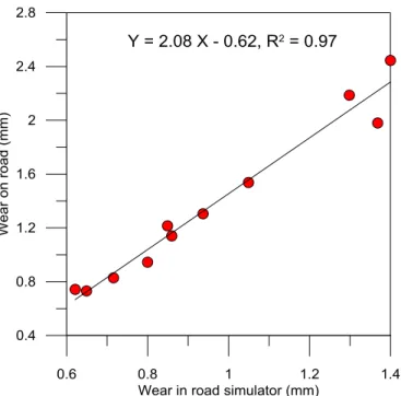
From wear studies it is well known that the wear in the simulator is accelerated but with a good correlation to test surfaces of the same pavements on real road (Jacobson och Wågberg, 2007). In Figure 2 results from a study where the wear of pavement slabs on roads was compared to the wear of the same pavement constructions in the road simulator. If the correlation is as high for PM10 is difficult to investigate, but previous studies show a good correlation between wear and

PM10 production (Gustafsson och Johansson, 2012) in the simulator, why it is reasonable to

(17)

Figure 2. Wear on a number of pavements slabs on roads compared to the wear of the same pavement constructions in the VTI road simulator. From (Jacobson och Wågberg, 2007).

2.2. Pavement

A pavement ring, used for a previous wear test, including 14 different asphalt pavements with different rocks, and constructions, tested for wear in a previous project was used for the tests.

Table 1. Pavement types in the ring used for the tests. SMA = stone mastic asphalt, AC = asphalt concrete, NBM = Nordic ball mill value.

1 SMA16 PMB KGO (polymer modified bitumen, flow mixed asphalt)

2 SMA16 GMB (rubber modified bitumen)

3 SMA16 100/150

4 SMA 16 70/100 +1% cement; ball mill value<7

5 SMA 11 GMB (rubber modified bitumen)

6 SMA 11 GMB LTA (rubber modified bitumen, low temperature asphalt)

7 SMA11 70/100

8 SMA 11 GMB KGO (rubber modified bitumen, flow mixed asphalt)

9 SMA 11 70/100

10 SMA11 PMB (polymer modified bitumen)

11 GAP11 KÅ (rubber pavement with size distribution gap, Kållered)

12 AC16 100/150 GMB NBM<5 (rubber modified bitumen, NBM<5)

13 AC16

(18)

2.3. Tyres and stud characteristics

Six studded tyres (dimension 205/55R16) on the market were chosen together with one tyre of an older type. The types and tyres tested were:

1. Studded tyres complying with current regulations in Norway today and regulations in Sweden and Finland before 1/7 2013. 130 studs

a. Nokian Hakkapeliitta 5

2. Studded tyres complying with regulations in Sweden and Finland after 1/7 2013, but has passed the over-run test. 130 studs

a. Pirelli Ice Zero

b. Goodyear Ultragrip Ice Arctic c. Continental Ice Contact

3. Studded tyres complying with new regulations in Sweden and Finland after 1/7 2013. 96 studs

a. Michelin X-Ice North b. Gislaved Nord Frost 100

4. Studded tyres that have passed the over-run test despite more studs that both old and new regulations. The only tyre not approved in Norway but with an exemption. 190 studs.

a. Nokian Hakkapeliitta 8

Tyre 4.a. is used as a reference tyre in the tests. The tyres and their studs are described in the following.

(19)

Figure 3. Stud appearance. From left to right: Nokian Hakkapeliitta 8, Nokian Hakkapeliitta 5, Continental, Goodyear, Gislaved, Michelin, Pirelli. Photos: Mats Gustafsson, VTI.

Figure 4. Mean weight of studs of the different tyres. Error bars are standard deviation. 0 0,2 0,4 0,6 0,8 1 1,2

(20)

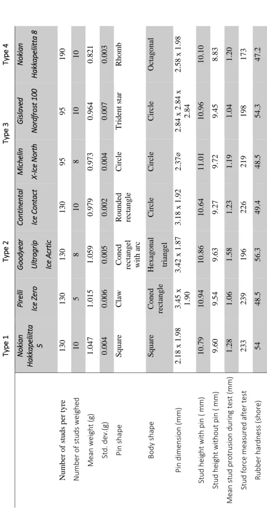
Table 2 St u d and tyr e pr o p er ti es . Ty p e 1 Ty p e 2 Ty pe 3 Ty pe 4 N o ki a n H a kk a pel iitt a 5 P ir el li Ic e Z er o G oo dy ea r U lt ra g ri p Ic e A crt ic C on ti n en ta l Ic e C o nta ct M ic hel in X-Ic e N ort h G is la ve d N ord fro st 10 0 N ok ia n H ak ka pel iitt a 8 N um ber of st u ds pe r ty re 130 130 130 130 95 95 190 N u mb er of s tu ds we ighe d 10 5 8 10 8 10 10 Mea n w ei ght ( g) 1.047 1.015 1.059 0.979 0.973 0.964 0.821 Std. de v. (g) 0.004 0.006 0.005 0.002 0.004 0.007 0.003 Pin shape Squar e C law C oned rec tang el w it h a rc R ounded rec tang le C ir cl e T ri de nt st ar R hom b Body s ha pe Squar e C oned rec tang le H exa g onal tr iang el C ir cl e C ir cl e C ir cl e O ct ag onal Pin dime ns ion ( mm ) 2.18 x 1.98 3.45 x 1.90 3.42 x 1.87 3.18 x 1.92 2.37 ⌀ 2.84 x 2.84 x 2.84 2.58 x 1.98 Stud he ight w ith pi n ( m m) 10.79 10.94 10.86 10.64 11.01 10.96 10.10 Stud he ight w ithout pin ( m m) 9.60 9.54 9.63 9.27 9.72 9.45 8.83 Mea n st ud pr otr us io n d ur in g te st ( mm ) 1.28 1.06 1.58 1.23 1.19 1.04 1.20 Stud fo rce m ea sur ed af te r te st 233 239 196 226 219 198 173 Rub be r h ar dn es s (s hor e) 54 48.5 56.3 49.4 48.5 54.3 47.2

(21)

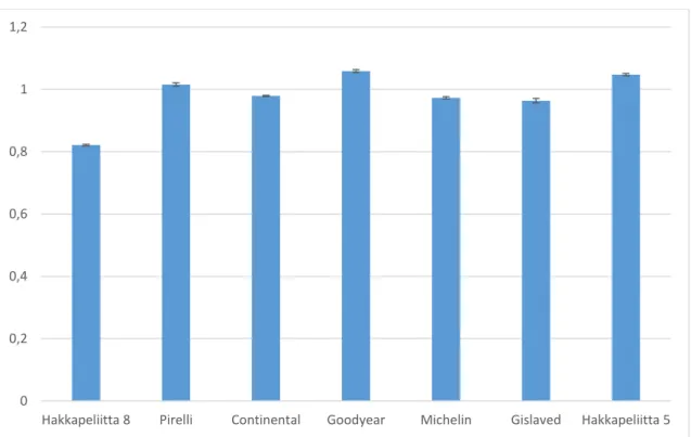
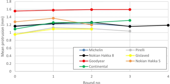
Stud protrusion was measured before and after each run (for procedure, see section 2.4). The mean values of 40 studs of each tyre set are presented in Figure 5. All tyres, except the

Goodyear tyre fluctuate around 1.2 mm protrusion. The Goodyear tyres are stable at around 1.6 mm protrusion.

Figure 5. Stud protrusion during measurements. Each point represents the mean value of 40 studs (10 studs measured on each of four tyres).

2.4. Test procedure

Before the very first day of the tests the simulator hall has been cleaned using a high pressure water cleaner. The hall is then dried and cooled to about 0º C. The pavement temperature is often slightly higher, but never higher than 2º C. Before every following test day, the hall is not cleaned with water again, but resuspension is minimized using compressed air blowing as described below.

Tyres are stored in room temperature outside the simulator hall. Two sets of rims are used to be able mount one set of tyres as another is tested. The test procedure is as follows:

1. Tyres are inflated to 2 bars

2. Stud protrusion is measured before mounting tyres on simulator (always the same ten studs on each tyre).

3. Tyres are mounted (always the same tyres on the same rim and axle) 4. Cooler is turned off

5. Simulator is started and accelerated to 50 km/h

6. After 1 hour, if PM10 level is constant or decreasing, simulator is stopped. If PM10 is

still rising, test is run until PM10 levels out.

7. Cooler and a large air filtering fan are started to reduce deposition and lower the PM10

concentration to initial level

8. Pavement track and tyres, when mounted on the simulator, are blown with compressed air to reduce resuspension of dust in the following test.

9. Tyres are switched to next set.

10. When PM10 concentration reaches initial level, cooler and air filtering fan are turned off

0 0.2 0.4 0.6 0.8 1 1.2 1.4 1.6 1.8 0 1 2 3 4 Me an p ro tru sion (mm ) Round no Michelin Pirelli

Nokian Hakka 8 Gislaved

Goodyear Nokian Hakka 5

(22)

2.5. Particle measurement

PM

10

and PM

2.5

air concentration

Regarding concentration of PM2.5 and PM10, three different techniques were used.

 Tapered Element Oscillating Microbalance (TEOM)

The instrument is based on gravimetric technique using a microbalance. A value of mass concentration PM10 is given every 5 minutes. The method is certified for air

quality standard monitoring within the EU.

 DustTrak (DT)

Two of these optical instruments were used during the measurements; one measured mass concentration PM2.5 and the other PM10. The time resolution of the sampling was 3

s for both instruments.

Particle size distributions

Particle size distributions describe how airborne particles are distributed in size according to mass and number (volume and surface area is also a possibility, but not of interest in this study). The size distributions were measured using an APS (aerodynamic particle sizer) model 3321 (TSI, USA) measuring mass distribution and an SMPS-system (scanning mobility particle sizer) model 3934 (TSI, USA) measuring number distribution. The SMPS-system was setup to measure and count particles from 7.37 nm to 311 nm. The APS was equipped with a PM10 inlet

and hence, measured particles with aerodynamic diameter from 0.523 to 10 µm. Size distributions of particles measured with the SMPS system are presented as number size

distributions and particles measured with the APS are presented as mass size distributions. This is because the fine fraction below 1 µm makes up very little of the mass but contain the majority of the particles while the coarser particles are very few, but dominate the mass concentration. When presenting data from APS and SMPS it is common to normalize the measured particle mass distribution. The normalization means that measured mass for a specific particle size range (=dM) is divided by the logarithm of the measured particles size interval = d log(dp) (often written as dlogDp). This means that mass distributions measured using instrument with different particle size intervals could easily be compared.

2.6. Statistical analysis of PM

10

, PM

2.5

and number concentration

data

The choice of an experimental design depends on the details of the analysis and vice versa and they need to be decided upon simultaneously. Here, we start by describing the analysis

procedure.

Analysis

For all analyses, a 15-minutes mean value of PM10 and number concentration at the end of each

simulator run was used. The data can be described as a sum of general behaviour, tyre effects and a random component. The general behaviour is specific for each day. It includes changes in the experimental environment that is assumed to have a linear shape during the day. That is supposed to include change in temperature and humidity but also any other drift with linear shape. The general behaviour can be modelled as straight lines, one for each day. Also, each tyre except the reference should be compared to the reference. The tyre effects, one for each tyre except the reference tyre, are not assumed to change between or within days and are modelled as constants.

(23)

A multiple linear regression was used to analyse general behaviour and tyre effects

simultaneously. The tyre effects, when comparing other tyres to the reference, are estimated in this analysis. Comparing other tyres than the reference to each other is also possible, though this cannot be immediately read as results from the analysis.

To explain the shape of the explanatory variables, think of a reduced experiment where data are collected for a reference tyre labelled A and 3 other tyres labelled B, C and D during 2 days. The order is described in Table 3.

Table 3. Order of tyres in a reduced experiment with a reference tyre and 3 other tyres.

Day Order during day

1 2 3 4 5

1 A B C D A

2 A C D B A

Because each day has its own intercept and slope, the model does not need to have a general intercept. A design matrix, a matrix that combines all the explanatory variables, for this analysis is: 𝑋 = ( 1 1 0 0 0 0 0 1 2 0 0 1 0 0 1 3 0 0 0 1 0 1 4 0 0 0 0 1 1 5 0 0 0 0 0 0 0 1 1 0 0 0 0 0 1 2 0 1 0 0 0 1 3 0 0 1 0 0 1 4 1 0 0 0 0 1 5 0 0 0)

The regression coefficients for columns 1 and 2 describe the general behaviour (intercept and slope) during day 1, the coefficients for columns 3 and 4 describe the general behaviour day 2 and the coefficients for columns 5 to 7 compares tyre B with A, C with A and D with A

respectively. Tyres B and C can be compared by comparing the coefficients for column 5 and 6 etc.

The reference tyre does not need to be tested each day. If a tyre E is also included in the reduced experiment, a possible design is described as in Table 4

.

Table 4. Order of tyres in a reduced experiment with a reference tyre and 4 other tyres.

Day Order during day

1 2 3 4 5

1

A B C D A

(24)

Though the design allows a comparison of E with A it may possibly not be very efficient for that comparison.

Design of experiment

It is not obvious which one is the most efficient of all possible experimental designs. The design needs to be found by first defining some quantity that measures efficiency in the analysis method and then find the best design according to this measure.

In the chosen analysis method, the differences between tyres and the reference tyre are expressed as regression coefficients. As a measure of efficiency we use the variance of these regression coefficients, with the goal to make these variances as small as possible. The variance of a regression coefficient is the product of the random variation times the corresponding diagonal element in the (𝑋𝑡 _{∙ 𝑋)}−1_{matrix. The first factor, the random variation, has a fixed}

expected value that cannot be changed by the design. However, one can choose the best in a set of suggested designs by finding the one that minimizes the second factor. Because the design must be allowed to be unbalanced, meaning that the variations of the regression coefficients becomes unequal, we chose the maximum of the diagonal elements in the (𝑋𝑡_{∙ 𝑋)}−1_{matrix as}

our measure of efficiency. This maximum is found over only those elements that represent tyre effects (elements representing general behaviour have been left out).

It was decided that the reference tyre should be used 4 times during the experiment while the other tyres should be used 3 or 2 times to avoid very different wearing of the tyres. We wanted to avoid two consecutive runs with the same tyre or any repeated sequence of tyres. Tough we have this restriction on the number of times each tyre should be used and we know how to compare possible designs, it is not straightforward to exactly figure out which one is the best. The solution was to search for the best design by scanning through a huge set of randomly generated designs. The design matrix was found the same way as in the examples above but with 20 rows and 14 columns. The first 8 columns corresponds to the general behaviour and the remaining 6 (numbered 9—14) corresponds to the coefficients comparing each tyre with the reference. A design for which 𝑋𝑡_{∙ 𝑋 does not have an inverse was immediately rejected. We}

chose the one that had the smallest maximum of diagonal elements 9—14 of the (𝑋𝑡_{∙ 𝑋)}−1

matrix. The results indicate that it is efficient to use the same tyre on the first and last run each day. Therefore, the random generating algorithm of designs was tuned to only scan through such designs and the search was restarted. The procedure does not guarantee that we found the best design, but it has a high probability that de design is at least close to being the best. The tyres were labelled 0—6 where 0 is the reference and the chosen design is shown in Table 5. The design does not have any repeated sequence. It allows comparisons between any pair of tyres though it is primarily chosen for comparisons with the reference.

Table 5. Chosen design for analyses.

Day Order during day

1 2 3 4 5

1 4 1 0 5 4

2 2 0 6 1 2

3 0 3 5 6 0

4 3 1 4 2 3

(25)

Statistical analyses of tyre properties and experimental environment

When choosing an analysis for this data, the difference between tyres can be thought of as only constants without any lower level structure or as a function of tyre properties that explains these differences. It is not generally possible to combine those analyses into one analysis with both tyre levels expressed as constants and tyre levels explained by tyre properties. In a similar way, general behaviour during days may be modelled as a shape without any other explanation to why that shape occurs, or it may be modelled as a function of variables that are supposed to have the ability to explain the particle emissions, but not generally both ways in one analysis. The analyses above quantify the difference between tyres without any attempt to find out how properties like stud weight may explain such differences. It also assumes a linear drift during days without trying to explain such a drift. In this section we model particle emissions as a function of tyre properties and variables describing the experimental environment. Multiple linear regression is used for this analysis.

The available explanatory variables are road temperature, air temperature, humidity, tyre temperature, speed, stud protrusion, number of studs, stud weight, rubber hardness and stud force. Some interactions can also be expected, possibly number of studs * stud weight and number of studs * stud force being the most obvious. However, it is advised that all these variables should not be used in the same analysis because using all of them results in multi-colinearity.

Comparing the statistical analysis procedures

For a comparison of the tyres “as is” without trying to explain the differences, the first approach is better. If the aim was to really find out how stud weight etcetera can explain particle

emissions, the second approach could be better, but only if no important explanatory variable has been left out. Some important explanatory variables, not included here, could be rubber compound, stud geometry, etc.

For the general behaviour, the first approach allows a drift during a day that may be modelled as a straight line. Possibly, a line is too simple and the analysis should allow a more complicated shape. The second approach can be better if changes in the environment should be explained in terms of changed wind speed etc. but, once again, only if no important variable has been left out. Also, the experiment is not designed to find the best estimates of the effects of changes in the environment variables. The environment is controlled to keep temperature etc. constant. To get better estimates one must allow, or even force, more variation in the environment.

It has been said above that it is not generally possible to combine the two types of analyses. If the explanatory variables are divided into an environment section and a tyre section, it is allowed to use one type in one section and the other type in the other section. An analysis using tyre effects as constants and air temperature etc. to describe the environment can be used. In this case, we are primarily interested in the comparing the tyres as is adjusting for change in the environment but we are not primarily interested in explaining the difference between tyres or finding estimates of the effects of air temperature etc. We chose primarily to use the first approach as a main analysis.

(26)

3. Results

The main focus of this study was to compare the production of PM10 particles from different

types of studded tyres, due to their importance for current PM10 limit values. Even though

studded tyres not are considered a problem for PM2.5 limit values particle number

concentrations, these data are also presented, since they are of general interest from a health point of view.

The studied tyres were:

Label Tyre

Colour code

in diagrams

0 Nokian Hakka 8

1 Pirelli

2 Goodyear

3 Continental

4 Michelin

5 Gislaved

6 Nokian Hakka 5

3.1. Statistical analyses of PM

10

, PM

2.5

and number concentration

Statistical analyses of PM

10

data

Test time series data for PM10 for all four test days are shown in figures in Appendix C. The

results of the regression analysis are shown in Table 6.

Table 6. Results of the regression analysis of PM10-data.

Estimate Std. Error t value P-value

Intercept day1

12.78

0.56

22.93

0.000 Slope day1

-0.43

0.15 -2.90

0.027 Intercept day2

11.92

0.51

23.48

0.000 Slope day2

-0.36

0.15 -2.47

0.048 Intercept day3

10.96

0.52

20.94

0.000 Slope day3

-0.24

0.15 -1.61

0.158 Intercept day4

9.62

0.58

16.59

0.000 Slope day4

0.14

0.15

0.94

0.385 Pirelli compared to ref

-2.55

0.40 -6.41

0.001 Goodyear compared to ref

-4.03

0.40 -10.04

0.000 Continental compared to ref

-2.75

0.40 -6.89

0.000 Michelin compared to ref

-3.82

0.40 -9.62

0.000 Gislaved compared to ref

-6.51

0.41 -15.92

0.000 Nokian Hakka 5 compared to ref

-1.77

0.41 -4.32

0.005

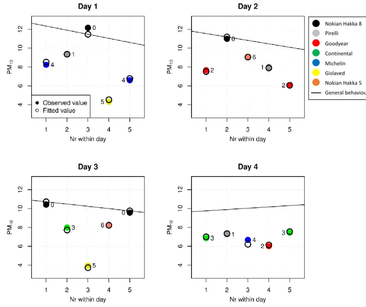
The PM10 data are shown in Figure 6. The bullets show the observations and the circles show

the fitted values. The vertical distances between circles and bullets are estimates of the random variation. The reference lines represent the general behaviour during the days, which is also the fitted emission for the reference tyre if it would have been tested on any day as any number within day.

(27)

Figure 6.Observed and fitted PM10 values with tyre labels for all days. Nokian Hakka 8 Pirelli Goodyear Continental Gislaved Nokian Hakka 5 Michelin General behaviour

(28)

The coefficients 9-14 describe the estimated differences between any other tyre and reference tyre (Nokian Hakkapeliitta 8). A negative sign shows that the other tyre has lower particle emission than the reference tyre. The reference tyre has an average particle emission of about 10 (Figure 6) and all other tyres have significantly lower emissions. The P-values in Table 6 are not adjusted for multiple comparisons. R2_{for this analysis is 0.985. R}2_{may be problematic in}

designs without a general intercept. R2_{was found in a model with a general intercept but}

without an intercept for day 1. This model gives the same estimates and inference for the tyre effects but uses another parametrization of the general behaviour.

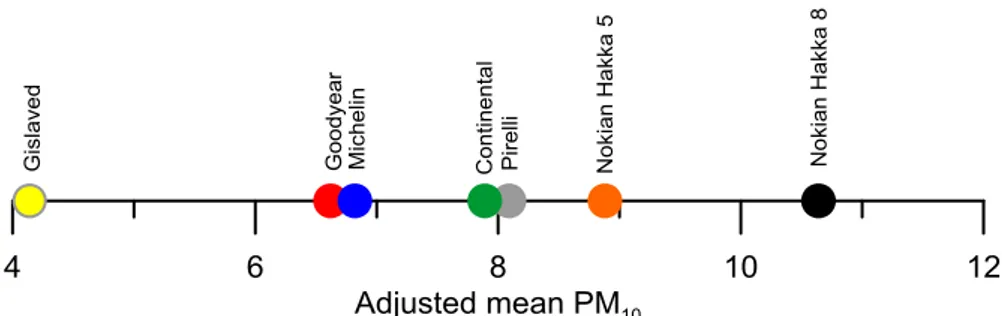
Table 7 shows the mean PM10 for each tyre. The sample means are averages of the observations

without any adjustment. These are simple estimates without any ability to adjust for the

assumed structure with general behaviour that vary between days. There are some differences in general behaviour between days and the tyres are not uniformly distributed between or within days. The differences between days should be adjusted for though they are small. The adjusted means represent the sample means after being adjusted for the varying general behaviour. That is an estimate of the mean if the tyre was tested an equal number of times each day,

symmetrically distributed within each day. For the reference tyre, the adjusted mean is found by taking the mean intercept for the four days plus the mean slope times 3 (3 is the middle of the order 1—5 within days). For the other tyres, the adjusted mean is found by also adding the estimated difference between that tyre and the reference tyre.

The fitted values in Figure 6 show the data after trying to remove only the random component while keeping tyre effects, day specific intercept and day specific slope, while the adjusted values in Table 7 show the data after also levelling out the difference in general behaviour between and within days. The fitted values are better to use when checking the underlying model assumptions. The adjusted values are easier to use for comparing the tyres.

Table 7. Mean PM10 values (in mg/m3) without and with adjustment for general behaviour.

Tyre Sample mean Adjusted mean

Type

Nokian Hakka 8

10.79

10.64

4 Pirelli

8.20

8.09

2 Goodyear

6.58

6.62

2 Continental

7.43

7.89

2 Michelin

7.17

6.82

3 Gislaved

4.13

4.14

3 Nokian Hakka 5

8.64

8.88

1

Looking at the results in order from highest to lowest emission, we observe that the tyres can be divided into 4 groups (Figure 7 and Table 8), where the tyres within groups do not differ significantly on 5 % level while the P-values between closest neighbours in groups are written in the list. P-values are not corrected for multiple comparisons.

(29)

Figure 7. Order of adjusted mean PM10.

Table 8. Significantly separated tyre groups for PM10 results.

Group Tyre

Type

1 Nokian Hakka 8 4

0.005

2 Nokian Hakka 5 1

2 Pirelli

2

2 Continental

2

0.043

3 Michelin

3

3 Goodyear

2

0.003

4 Gislaved

3

Table 9 gives difference (gray background) and unadjusted P-value (white background) in comparisons between pairs of tyres other than the reference. The difference is defined as the PM10-value for the tyre named by column name minus the value for the tyre named by the row

name.

Table 9. Differences in PM10 between tyres other than the reference and adjusted P-values.

Goody

ear

C

onti

ne

ntal

M

iche

li

n

Gisl

av

ed

N

ok

ian Hak

ka 5

Pirelli -1.47 -0.20 -1.27 -3.95

0.79 0.011 0.647 0.019 0.000 0.143

Goodyear

1.28 0.21 -2.48

2.26 0.024 0.657 0.003 0.002

Continental

-1.07 -3.75

0.99 0.043 0.000 0.088

Michelin

-2.68

2.06 0.001 0.006

Gislaved

4.74

0.000 Statistical analyses of PM

2.5

data

The data for PM2.5 have different level than PM10 but the assumed structure of the data is the

same and the data are collected from the same experimental design. It should be noted that the data used for PM2.5 is from an optical DustTrak instrument not considered as reliable as the

gravimetric TEOM instrument used for the PM10 analysis. We use the same analysis for number

(30)

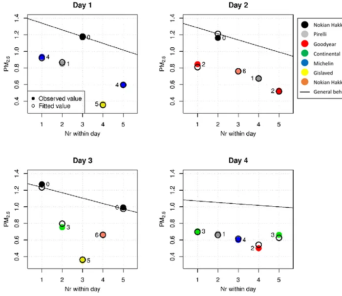
Figure 8 .Observed and fitted PM2.5 values with tyre labels for all days.

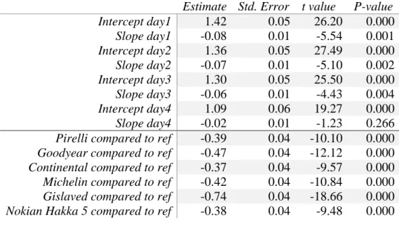
The results of the regression analysis are shown in Table 14. R2_{for this analysis was 0.991.}

Nokian Hakka 8 Pirelli Goodyear Continental Gislaved Nokian Hakka 5 Michelin General behaviour

(31)

Table 10. Results of the regression analysis of PM2.5

Estimate Std. Error t value

P-value

Intercept day1

1.42

0.05

26.20

0.000 Slope day1

-0.08

0.01 -5.54

0.001 Intercept day2

1.36

0.05

27.49

0.000 Slope day2

-0.07

0.01 -5.10

0.002 Intercept day3

1.30

0.05

25.50

0.000 Slope day3

-0.06

0.01 -4.43

0.004 Intercept day4

1.09

0.06

19.27

0.000 Slope day4

-0.02

0.01 -1.23

0.266 Pirelli compared to ref

-0.39

0.04 -10.10

0.000 Goodyear compared to ref

-0.47

0.04 -12.12

0.000 Continental compared to ref

-0.37

0.04 -9.57

0.000 Michelin compared to ref

-0.42

0.04 -10.84

0.000 Gislaved compared to ref

-0.74

0.04 -18.66

0.000 Nokian Hakka 5 compared to ref

-0.38

0.04 -9.48

0.000

The table of sample means and adjusted means are shown in Table 11.

Table 11. Mean PM2.5 without and with adjustment for general behaviour

Tyre Sample mean Adjusted mean

Type

Nokian Hakka 8

1.15

1.11

4 Pirelli

0.73

0.72

2 Goodyear

0.62

0.64

2 Continental

0.71

0.74

2 Michelin

0.71

0.70

3 Gislaved

0.36

0.37

3 Nokian Hakka 5

0.71

0.74

1

The order is not the same as for PM10 and that the tyres group differently. The tyres can be

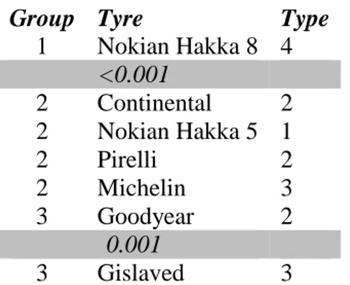
divided into 3 groups (Figure 9 and Table 12).

(32)

Table 12. Significantly separated tyre groups for PM2.5 results.

Group Tyre

Type

1 Nokian Hakka 8 4

<0.001

2 Continental

2

2 Nokian Hakka 5 1

2 Pirelli

2

2 Michelin

3

3 Goodyear

2

0.001

3 Gislaved

3 The P-value when comparing Continental and Goodyear is 0.04972 which is less than

0.05. Despite this, we have decided not to go into some deeper discussion about if these

tyres should be regarded as belonging to different groups.

Table 13 gives differences and unadjusted P-values when comparing tyres other than the reference in pairs.

Table 13. Differences in PM2.5 between tyres other than the reference and adjusted P-values.

Goody

ear

C

onti

ne

ntal

M

iche

li

n

Gisl

av

ed

N

ok

ian Hak

ka 5

Pirelli

_{-0.082 0.019 -0.027 -0.350 0.014} 0.085 0.646 0.503 0.000 0.762

Goodyear

_{0.101 0.054} _{-0.268 0.096} 0.050 0.255 0.001 0.070

Continental

_{-0.047 -0.370 -0.005} 0.293 0.000 0.920

Michelin

_{-0.323 0.042} 0.000 0.418

Gislaved

_0.365 0.000

(33)

Statistical analyses of number concentration

The data for number concentration of particles have different level than PM10 but the assumed

structure of the data is the same and the data are collected from the same experimental design. We use the same analysis for number concentration as for PM10 data and show the results with

the same figures and tables.

The number concentration data are shown in Figure 10.

Figure 10. Observed and fitted concentrations with tyre labels for all days

The results of the regression analysis are shown in Table 14. R2_{for this analysis was 0.965.}

Nokian Hakka 8 Pirelli Goodyear Continental Gislaved Nokian Hakka 5 Michelin General behaviour

(34)

Table 14. Results of the regression analysis of number concentration.

Estimate Std. Error t value P-value

Intercept day1

127668

9553

13.36

0.000 Slope day1

-308

2568

-0.12

0.908 Intercept day2

135203

8701

15.54

0.000 Slope day2

-4784

2528

-1.89

0.107 Intercept day3

118696

8973

13.23

0.000 Slope day3

-2594

2572

-1.01

0.352 Intercept day4

109781

9943

11.04

0.000 Slope day4

-926

2532

-0.37

0.727 Pirelli compared to ref

1177

6832

0.17

0.869 Goodyear compared to ref

-15490

6878

-2.25

0.065 Continental compared to ref

-11877

6848

-1.73

0.134 Michelin compared to ref

-43794

6808

-6.43

0.001 Gislaved compared to ref

-65745

7002

-9.39

0.000 Nokian Hakka 5 compared to ref

-15080

7008

-2.15

0.075

The table of sample means and adjusted means are shown in Table 15.

Table 15. Mean number concentration without and with adjustment for general behavor.

Tyre Sample mean Adjusted mean

Type

Nokian Hakka 8

118552

116378

4 Pirelli

118193

117555

2 Goodyear

100436

100888

2 Continental

97294

104501

2 Michelin

76369

72583

3 Gislaved

52930

50633

3 Nokian Hakka 5

99505

101297

1

The order is not the same as for PM10 and the tyres group differently. The tyres can be divided

into 3 groups (Figure 11 and Table 16).

(35)

Table 16. Significantly separated tyre groups for number concentartion results.

Group Tyre

Type

1 Pirelli

2

1 Nokian Hakka 8 4

1 Continental

2

1 Nokian Hakka 5 1

1 Goodyear

2

0.010

2 Michelin

3

0.029

3 Gislaved

3

Table 17 gives difference and unadjusted P-value when comparing tyres other than the reference in pairs.

Table 17. Differences in number concentration between tyres other than the reference and adjusted P-values.

Goody

ear

C

onti

ne

ntal

M

iche

li

n

Gisl

av

ed

N

ok

ian Hak

ka 5

Pirelli

_{-16667 -13054 -44971 -66922 -16257} 0.054 0.114 0.001 0.000 0.089

Goodyear

₃₆₁₃ _{-28304 -50255 410} 0.637 0.010 0.001 0.959

Continental

_{-31917 -53868 -3203} 0.004 0.001 0.713

Michelin

_{-21951 28714} 0.029 0.015

Gislaved

₅₀₆₆₅ 0.001

Results for tyre properties and experimental environment

(36)

Table 18. Results of statistical analysis of parameters influencing PM10.

Estimate Std.Error P(>|t|)

₎

_-0.709

_0.247

_0.017

Speed (mg m

-3

km/h

-1

)

0.298

0.460

0.532 Mean protrusion during test (mg m

-3

_mm

-1

₎

_2.273

_1.423

_0.141

Number of studs (mg m

-3

stud

-1

)

0.047

0.010

0.001 Stud force (mg m

-3

N

-1

)

0.037

0.009

0.002 Rubber hardness (mg m

-3

shore

-1

)

-0.133

0.075

0.107

R2_{for this analysis is 0.952. The first set of variables describes the environment. Three}

significant result can be seen, that PM10 emission increase with higher air temperature and

humidity and decrease with higher tyre temperature. The second set of variables describes the tyres. Emissions increase with higher number of studs and higher stud force, and decrease with higher rubber hardness (not significantly, though). Possibly, the studs wearing of the surface should be expressed as the number of studs times the stud force, but adding this interaction to the model did not improve the explanation significantly.

Two types of analyses have been done here. The first type only models tyre effects as constants, the second tries to describe the tyre effects as a function of stud weight etc. Both have high R2_,

indicating that both models fit good to the data. Also, in Figure 6 and Figure 10, the similarity in level and pattern between circles and bullets indicate that the model fits well and has the same structure as the data.

For PM2.5, the result of the regression analysis is presented in Table 19. Table 19. Results of statistical analysis of parameters influencing PM2.5.

Estimate Std.Error P(>|t|)

₎

₎

_-0.020

_0.009

_0.055

The results are similar in shape as PM

10

. R

2

for this analysis was 0.954. Compared to

PM

10

, road temperature has become significant while tyre temperature has lost its

significant result. There are one significant tyre variable coefficient, the number of

studs. The analysis did not improve significantly when adding interaction between stud

force and number of studs. The size of the coefficients cannot easily be compared with

the coefficients in the analysis of PM

10

data because PM

10

and PM

2.5

have totally

different levels.

(37)

For concentration, a model that does not use stud force or any interactions is supported by the data and does not leave any obviously important variable out. The result of the regression analysis is presented in Table 20.

Table 20. Results of statistical analysis of parameters influencing number concentration..

Estimate Std.Error P(>|t|)

(Intercept) -611686

286282

0.058 Road temp (# m

-3

Cº

-1

)

-14588

13740

0.313 Air temp (# m

-3

_Cº

-1

₎

₁₃₀₃₁

concentration have totally different levels.

3.2. PM

10

size distributions

Mass size distributions from APS instrument

The APS instrument is not a gravimetric method and uses the aerodynamic diameter considering all particles as spherical. Also a particle density must be set from assumptions or measurements. In this experiment, the particle source is of constant composition why comparison between concentrations and size distributions can be made. During the first day an error (probably a larger dust particle that disturbed the nozzle) corrupted the data that could not be used for analyses.

The geometric mean size of the particles from the tyres are fluctuating around 4 µm. The Continental and Goodyear tyres tended to produce slightly smaller particles with each proceeding test, but this is not a general trend (Figure 12).

(38)

Figure 12 Geometric mean size of particles analyzed using the APS instrument.

As can be seen in Figure 13, mass size distributions are similar and seem to be bi-modal (or even tri-modal), with mass peaks at 2-3 µm, 4-5 µm and one at 7-8 µm close to the PM10

cut-off. Generally, the coarser modes seem to contribute relatively more in the first test with each tyre and become weaker at later tests, while the finer mode seems is relatively less affected by repeated tests. This behaviour is most obvious in the type 2 tyres, while the size distributions for the Nokian Hakkapellitta tyres in type 1 and 4 do not change much from test to test. Being a complex test pavement, it is likely that the modes are associated with different pavement rocks with different wear resistances.

0 1 2 3 4 5 G eo. m ean (µm)

(39)

Figure 13. Mass size distributions during 15 minutes before each test stop. Legend numbers refer to “testday:tyre test number during day”.

T

y

pe

1 T

y

pe

2 T

y

pe

4 T

y

pe

3

(40)

Plotting the time series of mass size distributions reveals an initial decrease in particle size in each run, probably reflecting some initial resuspension before a balance between production and deposition is reached (Figure 14 and Figure 15).

(41)

Figure 15. Time series of mass size distributions from the APS instrument during day 4.

From the APS data the proportion of PM2.5 has been calculated and is shown in Figure 16. The

mean is 24 %.

Figure 16. Proportion of PM10 that is PM2.5.

Number size distributions from SMPS instrument

PM10 is a mass based measure, why coarser particles within the size fraction are contributing

0% 5% 10% 15% 20% 25% 30% % P M2.5 o f P M10

(42)

not regulated by environmental quality standards, but might be at least as important from a health point of view.

The geometric mean size is generally around 25 nm, except for the Gislaved and Michelin tyres, which generate slightly smaller particles at just above 20 nm (Figure 17).

Figure 17. Geometric mean size of ultrafine particles analyzed using the SMPS system.

In Figure 18, number size distributions from the tests are shown. The distributions are uni-modal, with a maximum number peak at 20-40 nm. All tyres have geometric mean particle size at approximately 25 nm, but for the Michelin and Gislaved tyres, the mean size is 22 and 20 nm, respectively. As for the APS distributions, but with some more data to support this result, the Michelin and especially the Gislaved tyres, produce lower number concentrations of ultrafine particles than the other tyres.

Studying the temporal evolvement of the number size distributions, a particle size growth can be seen during each test. This is a result of ultrafine particles agglomerating into larger aggregates. The size distribution development is similar for all tyres, but on different concentration levels.

0.00 5.00 10.00 15.00 20.00 25.00 30.00 G eo . m ean (n m )

(43)

Figure 18 Mean number size distributions during 15 minutes before each test stop. Legend numbers refer to “testday:tyre test number during day”.

T

y

pe

1 T

y

pe

2 T

y

pe

4 T

y

pe

3

(44)

Figure 19. Time series of number size distributions from the SMPS instrument during days 1 and 2.

(45)

Figure 20. Time series of number size distributions from the SMPS instrument during days 3 and 4. The extreme values the first minutes of day 4 is due to an erroneous setting of the SMPS.

3.3. Estimation of implications for air quality

Laboratory results in a road simulator are, naturally, not directly applicable for estimating effects on air quality in cities by changing type of studded tyre. Using the NORTRIP emission model, where road wear is included together with meteorological, road operation and traffic

(46)

been in use for some years. Despite the ban, the studded tyre use is about 30% during the winter season. In the rest of Stockholm the figure is about 50%. The modelled PM10 concentrations in a

situation where everyone using studded tyres used the lowest and the highest emitting tyres in this study is shown in comparison to the observed and the modelled reference concentrations. The modelled reference is what the wear and resulting PM10 emission that the model produces

when using standards settings for studded tyre use and wear. The highest emitting tyre has about 2.6 times higher PM10 emission than the lowest emitting tyre. The modelled reference is the

wear used in the model. If the reference road wear is assumed to be on a level right between the results of the tyres used in this test, the highest emitting tyre is 1.6 times higher than the

reference and the lowest emitting tyre 1.6 times lower. Figure 21 show the results of this calculation on the mean total PM10 concentration and the number of exceedances of the PM10

directive during October – May. The increase in net (only the local contribution of PM10 from

the street environment) and mean total (including background PM10) PM10 concentration is 41

and 22 % respectively compared to the reference case and the limit value is exceed 17 more days. The corresponding decrease is 25 and 14% and 18 exceedance days less.

(47)

20.4

18.4

25.9

13.7

Mean net concentration PM₁₀(ug/m3₎

Oct 2012 -May 2013 Hornsgatan

Observed Reference Stud wear x 1.61 Stud wear / 1.61

36.4

34.4

42.0

29.7