Mathematical description of railway alignments and some preliminary comparative studies

(1)

Mathematical description

of railway alignments and some

preliminary comparative studies

ij'rn Kufver

h

m

6)

Fl

<

9..

N

v I

L-c

a.

as

_h '5, 1 3E 9* 7?,r rej , 1 V7 * 7

*

Swedish National Road and

SWEDISH TRANSPORT

(2)

VTI rapport 420A - 1997

Mathematical description of railway alignments and some

preliminary comparative studies

ij'rn Kufver

Swedish National Road and

(3)

(4)

Publisher: Publication

VTI Rapport 420A

Published Project code

Swedish National Road and 1997 70041

' anspart Research Institute

Project

Optimisation of track geometry

Author Sponsor

Bj 6m Kufver Adtranz Sweden, SwedishNational Rail Administration

(BV), Swedish State Railways (SJ), Swedish Transport and Communications Research Board (KFB) and Swedish National Road and Transport Research Institute (VTI)

Title

Mathematical description of railway alignments and some preliminary comparative studies

Abstract

This report consists of two parts. The first part defines certain characteristics of railway alignments and introduces the use of curvature and slew diagrams for evaluating and comparing alignments.

In the second part, a base is formed to compare equally costly alignment alternatives. A parametric representation of the alignment is introduced. The axes in the parametric representation consist of the variables to be evaluated, and within the space (with at least two dimensions) boundary conditions are defined which are related to obstacles along the alignment. Comparisons without such boundary conditions cannot be regarded as being based on equal costs. The comparisons in this document are regarded as preliminary since the vehicle reactions are not adequately predicted.

Three sets of alignment problems are discussed in detail. First, the choice of radius and length of transition curve for a single curve between two straight lines is analysed. With the help of slew diagrams, it is concluded that a binding obstacle in the middle of the curve and a binding obstacle on the connecting straight line define two extremes where a lengthening of the transition curves requires the smallest and the largest compensation respectively in the curve radius.

With the positions of the obstacles in mind, different types of transition curves are evaluated and compared. The first, second and third derivatives of curvature are calculated and related to the associated lateral shifts and the shortenings of adjacent elements.

Finally, the horizontal alignment in crossovers is discussed. When different curvature patterns are compared, the boundary condition should define the length of the entire crossover (at a predefined lateral distance between the through tracks).

ISSN: Language: No. of pages:

(5)

(6)

Preface

This work has been carried out at the Division ofRailway Technology, Department of Vehicle Engineering, Royal Institute of Technology (KTH), Stockholm and the Railway Systems Group, Division of Transport Systems, Swedish Road and Transport Research Institute (VTI), Linkoping.

The work is part of the joint project concerning track/vehicle interaction commissioned by Adtranz Sweden, the Swedish National Rail Administration (Banverket), the

Swedish Transport and Communications Research Board (KFB), the National Swedish

Board for Technical and Industrial Development (NUTEK), the Swedish State Railways (SJ) and the Swedish National Road and Transport Research Institute (VTI).

The financial support provided by Adtranz Sweden, Banverket, KFB, SJ, and VTI for the present work is gratefully acknowledged. Parts of the present work have been developed for the Nordic Seminar on Track Technology, Swederail seminars and courses at Banverket s Railway Training Centre (Banskolan). Hence, also the Danish State Railways (DSB), Finnish State Railways (VR), Norwegian State Railways (NSB), Swederail AB and Banskolan have contributed to the financing of this report.

I would also like to thank Professor Evert Andersson at KTH for his support during the course of the work.

Linkoping, May 1997

Cover photo: Up line 1 and up line 2 of the Northern Main Line/Arlanda Line, Sollentuna. The bridge andplatform are binding lateral obstacles.

KTH TRITA FKT Report 1997:30 VTI Rapport 420A

(7)

KTH TRITA-FKT Report 1997230 VTI Rapport 420A

(8)

References

₆₉

Appendix 1 Terminology

Appendix 2 Notations

Appendix 3 Computer drawn curvature and slew diagram

(9)

KTH TRITA FKT Report 1997230 VTI Rapport 420A

(10)

Summary

This report consists of two parts. The first part defines certain characteristics of railway alignments and introduces the use of curvature and slew diagrams for evaluating and comparing alignments.

In the second part, a base is formed to compare equally costly alignment alternatives. A parametric representation of the alignment is introduced. The axes in the parametric

representation consist of the variables to be evaluated, and within the space (with at

least two dimensions) boundary conditions are defined which are related to obstacles along the alignment. Comparisons without such boundary conditions cannot be regarded as being based on equal costs. The comparisons in this document are regarded as preliminary since the vehicle reactions are not adequately predicted.

Three sets of alignment problems are discussed in detail. First, the choice of radius and length of transition curve for a single curve between two straight lines is analysed. With the help of slew diagrams, it is concluded that a binding obstacle in the middle of the curve and a binding obstacle on the connecting straight line define two extremes where a lengthening of the transition curves requires the smallest and the largest compensation respectively in the curve radius. The necessary compensation in curve radius also depends on the angle between the two straight lines.

With the positions of the obstacles in mind, different types of transition curves are

evaluated and compared. The first, second and third derivatives of curvature are

calculated and related to the associated lateral shifts and the shortenings of adjacent elements. The derivatives of the curvature might be expected to be correlated to the lateral jerk and its derivatives in the vehicle body, even though these relations are complex.

When binding lateral obstacles are placed in the adjacent elements, the derivatives should be related to the lateral shift. When a longitudinal obstacle (turnout) is placed in

an adjacent element, the derivatives should be related to the shortening of the adjacent element. It is concluded that a simplified version of the transition curve according to Ruch gives the lowest values of the first and second derivatives of curvature, both when the derivatives are related to lateral shifts and shortenings of adjacent elements respectively. In this comparison, the clothoid and the Helmert curve are regarded as special cases of the Ruch curve. With the Ruch curve, it is also easier to balance the magnitudes of the first and second derivatives of curvature. The Ruch curve and the clothoid are also more convenient (compared with other types of transition curves) for defining geometries in elements connected to the branch line of a curved turnout.

Finally, the horizontal alignment in crossovers is discussed. When different curvature patterns are compared, the boundary condition should define the length of the entire

crossover (at a predefined lateral distance between the through tracks). With such an

approach, it is obvious that turnouts with a transition curve at the heel in the branch line do not necessarily require a smaller radius in the main part of the turnout curve, as stated by others. The benefit of such a transition curve must be evaluated with simulations (or full scale testing) of vehicle reactions.

KTH TRITA-FKT Report 1997:30 i

(11)

On the other hand, if a transition curve is placed at the tip of a turnout, this transition curve will require a reduction of the radius. Hence, the advantage of these transition curves is assumed to be smaller compared to the advantage of those in the middle part of the crossover.

Keywords: Alignment, track geometry, transition curve, turnout, crossover, curvature,

track irregularity, misalignment, slew, lining machine, regression analysis, acceleration, jerk, passenger comfort.

ii KTH TRITA-FKT Report 1997230

(12)

PART I INTRODUCTION

1. Background

This report is one of a number in a project concerning optimisation of the alignment of railways. Railway alignment has a high degree of permanence. Installations such as

track superstructure, catenary system etc., are less permanent since these subsystems are

commonly renewed without alteration of the alignment. When building new lines,

obstacles along the route are relatively few, and the available terrain corridor should be

used in the best possible way to adapt the alignment for future requirements.

In track renewals, the number of obstacles along the railway is higher, since these include the original obstacles plus the railway-specific installations (such as catenary masts, bridges etc.) along the railway. Therefore, the possibilities of improving the

alignment are limited. However, insight into design (as shown by Baluch 1982, 1983, Hashimoto 1989, Schramm 1977, and Weigend 1988) should nevertheless enable

improvements to be made.

Analysis of the alignment improvements involves several areas of science. The evaluation of passenger comfort is analysed in Kufver (1997a) and the evaluation of track/vehicle interaction is analysed in Kufver (1997b). In this report, the geometrical basis for comparing alignments will be analysed.

When designing a curve between two straight lines, or a crossover between two adjacent

tracks, there are an infinite number of element combinations which can be used. It is not

possible to evaluate all these combinations. Also, if the alignment alternatives are chosen arbitrarily, this might lead to the wrong conclusion.

Some type of boundary condition must be introduced to make the comparisons meaningful and relevant. Two curve combinations which are compared should have the same lateral position in at least one cross-section of the line (where an obstacle is assumed to be placed). If two alignment alternatives can pass the same obstacles, they are assumed to be equally expensive to build. In order to enable general conclusions to

be drawn, the cross-sections where all the alternatives have the same lateral position

must be chosen with care. Such comparisons are analysed in Chapters 7 and 8.

At another level of optimisation, it might be interesting to compare alignment alternatives which do not fulfil the same boundary conditions, for example one alternative which passes an existing installation and another alternative which requires the installation to be removed. In such an analysis, it seems reasonable to compare the best alignment alternative fulfilling the boundary condition in question with the best alignment alternative where the condition is relaxed (derived with the methods in this

document). Such higher level comparisons, which show the net improvement

achievable at a higher cost, will not be discussed further in this document.

When different curvature patterns in a crossover are analysed, it seems reasonable to compare crossover alternatives with equal lengths (at a predefined track spacing). Such comparisons will be discussed in Chapter 9.

KTH TRITA-FKT Report 1997230 1

(13)

Earlier studies in the area of track alignments have not fulfilled these conditions. For example ORE (1974, 1976) sought to compare crossovers with radius 2000 m but lacking transition curves with crossovers with radius 2300 m and relatively long transition curves. As will be shown in Chapter 9, these comparisons cannot be regarded as relevant (if the purpose is to evaluate the net effect of the use of transition curves). Kruse (1984) compared existing alignments with the traditional type of transition curves (the clothoid) with alignments with an other type of transition curve. However, he did not use boundary conditions related to the position of the track. He noted that his type of alignment elements requires insignificantly more space than traditional alignments

elements and claimed that a sufficient solution would still be achieved. However, this

argument does not hold. It is obvious that the clothoid alternatives could have been improved and therefore his comparisons are irrelevant to the present study. Also, in the absence of boundary conditions related to the position, some of the alignments with clothoids, with which he compares his own layouts, are remarkably poor (since they have unnecessary compound curves and unnecessarily short clothoids).

Herbst et a1 (1987) used a few boundary conditions when they optimised the alignment with an advanced type of transition curve (the cosine curve). In one of their examples, with 6 fixed points, they used 4 straight lines (2 with zero length), 7 circular curves and 11 transition curves (2 with zero length) for the clothoid alternative. For the cosine curve alternative, they used 2 straight lines, 6 circular curves (all with zero length) and 7 transition curves. It seems very odd that they used so many degrees of freedom for the clothoid alternative and it is obvious that with these very few fixed points, the clothoid

alternative could have been improved. The criticism reported in Gurr (1988), that

2 transition curves have zero length and that the minimum radius was 190 m (instead of the 210 m in the cosine curve alternative), proves nothing since the clothoid alternative was not optimised.

Also Broman (1982) compared the traditional transition curve (the clothoid) with a new

type of transition curve (the p-curve). However, his boundary conditions do not seem relevant for road and railway design in practice. When justifying the need for a new type of transition curve, he forced the length of an adjacent straight line to a predefined value, instead of using a minimum length. In another comparison between the clothoid and his p-curve, he forced the length of a circular curve to be zero. If this condition is relaxed (by allowing a positive length of the circle), a clothoid alternative can be designed with both smaller curvature and smaller first derivative of curvature than the

p-curve alternative, and the conclusion of Broman would not hold.

However, Hashimoto (1989) has used relevant comparisons. For example, hestudied

alternatives where the alternative with a longer transition curve had a smaller radius in

the circular portion. However, since the necessary reduction of radius, depends on the

angle between the adjacent straight lines, it is not clear whether or not the relatively few comparisons he presented can lead to general conclusions.

In order to create a sound basis for the comparisons of alignments, the analysis of slew diagrams is carefully introduced in Chapter 4, and the use of a parametric representation of the alignment (R-Lt plane and R Ls plane respectively) is introduced in Chapter 7 and used in Chapters 7 and 9.

2 KTH TRITA FKT Report 1997230

(14)

It must be pointed out that the comparisons in this report are to be regarded as preliminary. The reason for this is that the vehicle reactions are not adequately predicted and that the criteria for track/vehicle interaction discussed in Kufver (1997a, 1997b) are not used.

KTH TRITA FKT Report 1997:30 3

(15)

(16)

2. Definitions

Track alignment refers to the designed position of the centre line of the track.

In this document the Cartesian coordinates x, y and z are defined according to Swedish surveying standards. The x coordinate runs in the northward direction and the y coordinate runs in the eastward direction. Both are expressed in metres. The direction

of the track, ([1 , is defined as zero if the track runs in the northward direction and is

defined clockwise if not. In Sweden, the direction is normally expressed in grades, but in this document the direction will be expressed in radians in order to simplify the equations.

The height of the track is defined by a z coordinate expressed in metres and the z-direction is upwards. (The x-y-z coordinate system constitutes a left hand coordinate system.)

The coordinates x, y and z, are normally expressed as functions of a chainage s, which runs in a horizontal projection of the alignment. The chainage is also expressed in

metres.

The trajectory in the horizontal plane of the mass centre line of a vehicle is in uenced by the cant D. When the superelevation is calculated as an angle, the lateral distance

between wheel rail contact patches is assumed to be 1500 mm, which corresponds to a

standard gauge of 1435 mm.

Curve radius R is positive for both right and left hand curves. Curvature k is positive for right hand curves and negative for left hand curves. In certain comparisons of derivatives, the magnitude is of interest, but not the sign. Therefore, k (s) is used in this

, , d k S

document to express the absolute value of the derivative of curvature d( ) . s

The relations which are described in this document are general. It does not matter whether the surveying of the track is performed with geodetic methods or other methods. If the track is measured with the versine method, manually or with track recording cars, the versines can easily be transformed into a set of local coordinates

(Kufver 1995a).

(17)

(18)

3. Differential equations for the direction w and the

coordinates x and y

3.1 General expressions and equations for straight lines and circular

curves

Figure 3.1 shows an arbitrarily curved track. The direction 90(5) can be calculated by

integration of the curvature k(s), which follows from the definition of radians

mm) = Jolt/1: jk(s)ds

[3.1]

{X(S), Y(S)}

Figure 3.1 An arbitrarily curved track in the x-yplane.

The coordinates {x(s), y(s)} for the alignment may then be calculated by double

integration

x(s) = J. cos w(s)ds = JcosJ k(s)ds ds

[3.2]

y(s) = J sin l//(S) dS = JsinJ k(s) ds ds [3.3]

These integrals can be solved analytically if the track is placed in a straight line or in a

circle. In these cases the curvature k(S) has a constant value. When the track is placed on

KTH TRITA FKT Report 1997130 7

(19)

a transition curve with a mathematical form used in railway applications, these integrals must be calculated with numerical methods. There are many computer programs

available for solving the equations involved, such as STEPP and DRD90 from the

Swedish National Road Administration and TOPORAIL from the Swiss Federal Railways. Typically, the coordinates are calculated with an accuracy of residual errors smaller than 10 3 m and the errors thus have no practical in uence in road and railway applications. Algorithms which are not difficult to implement in a computer have been

published by Broman (1982), Furmetz (1985a, 1985b) and Schuhr (1979a, 1979b, 1980,

1981, 1984, 1985, 1986).

However, there are many situations where track engineers must analyse and discuss different alignment alternatives, without having to calculate the alternatives with good accuracy using a computer. This will also be done in this document since the aim is to make general comparisons between different alignments, and these comparisons will be significantly easier if we make some approximations. In this document, the track geometry will usually be calculated approximately according to the assumption of small angles. If the track is not running northward in the global coordinate system, it is of course always possible to define a local coordinate system in which the track is running approximately in the x-direction.

When assuming small angles (1,0 << 1) the following approximations can be made

sin 1,0 z w z tan (,0 [3.4]

cos 1p z 1 [3.5]

If the curvature is zero, which corresponds to a straight line, the solutions to [3.1], [3.2] and [3.3] are

u =1/20

[3.6]

x=x0 +S-COSl/lo _[3,7] y=y0 +S°Sin {/10 [3.8] if IMO): I//() 13-9]

x(0) = x0

[3.10]

y(0)= yo

[311]

If the curvature is non zero but constant, which corresponds to a circular curve, the solutions to [3.1], [3.2] and [3.3] are

w=w0+k-s [3.12]

8 KTH TRITA-FKT Report 1997230

(20)

x = x0 + I: - (sin(w0 + k - s) Sin(l//0

[3.13]

1

y 2 yo + E - (COS(l//0) cos(l//0 + k - S»

_[314]

According to the assumption of small angles, approximate solutions to equations [3.1],

[3.2] and [3.3] applied to a circle are

l//(s) =[kds =w0+k-S

[3.15]

x(s)=Icost/l(s)dsz[1ds=x0+s [3.16]

S2

y(s) = JSi l/(S) dszj dedS =I(w0 +k-s)ds=y0 + WC -s+k-3 [3.17] Taylor expansions of equations [3.12] - [3.14] give the same results.

The integration constants 1,00, x0 and y0 may be eliminated by using an appropriate local chainage and appropriate local coordinates.

3.2 Some remarks about transition curves

Transition curves are normally inserted between two elements with constant curvature in order to avoid discontinuities in the curvature function along the alignment. (Such

discontinuities create unfavourable vehicle reactions.) The curvature within the transition normally starts with the same value, k0, as in the adjacent element before the

transition curve, changes continuously and ends with the same value as in the immediately following element, k1.

An interesting quantity of a transition curve is the absolute value of the derivative of

curvature, k (s) , which is defined as 'dk(s)

k (s) :1 ds

[3.18]

There are also types of transition curves where the second derivative k (s) and the third

derivative k (s) have finite values, within the transition curves as well as at the tangent

points. When these types of transitions are evaluated, it is also interesting to investigate the magnitude of these high order derivatives. Such investigations are made in Chapter 8.

The disadvantages with transition curves are a necessary lateral shift of one of the adjacent elements, w, and the fact that the transition curves replace parts of the adjacent elements. The lateral shift, w, and the necessary shortenings of adjacent elements will be derived in Section 3.3 and Chapter 8.

(21)

3.3 Equations for the clothoid

The most common type of transition curve is the clothoid. This type of transition curve is also called a cornu spiral and is often approximated as a third degree parabola.1 The third degree parabola was suggested by Pressel as early as 1854 (Schuhr 1985) and was

first used in the construction of Brennerbahn in 1864 1867 (Weber 1990).

In the clothoid, the curvature is a linear function of chainage S

k(s)=k0+Az [3.19]

if s = so = 0 at the start of the transition curve.

In equation [3.19] A is a constant. The nominator A2 may have a positive or a negative sign. The (positive) root of the magnitude of A2 is often called the clothoid parameter. If

the clothoid starts from a straight line (k0=0), has the length Lt (t = transition) and ends

at a circle with the radius R, we will have the following relation

[A2] = Lt - R

[3.20]

The absolute value of derivative of curvature k (s) is constant within the clothoid

1 A2

k1 k0

Lt

k' = [3.21]

Since the derivative of curvature, k (s), is not a continuous function at the tangent points where the clothoid starts and ends, the higher order derivatives of curvature

(k (s), k (s) etc.) are not defined.

Equation [3.19] combined with equations [3.1] and [3.3] - [3.4] gives

2

w(s)=[k(s)ds=[[k0+Ejds=w0+k0s+2i42

[3.22]

2

y(s) z [sin w(s) ds z Hk(s)dsds = [(1% + k0 os+ 2:12st

32 s3

= + . + k . +

for 0 _<_ s S Lt .

Here, chains of elements with and without clothoids are compared. The first chain consists of two elements, with length L0 and curvature k0, and length L1 and curvature k1 respectively. The chainage is defined with s = 0 at the beginning of element 0 and the

1 A parabola is by definition a second degree curve, but in the railway sector the expression third degree parabola is commonly used for a third degree polynomial.

(22)

coordinate system is defined with x = O, y = O and 1/2 = 0 at the same point. With these definitions and the assumption of small angles, we will obtain the following stationing and coordinates at the end of element 1

s 2 L0 + L1 [3.24]

x z L0 + Ll

k k

yzEQ.L(2)+kO.LO.Ll+_2l.L%

_[3.26]

W :kO'LO +k1'L1 [3.27]

With an inserted clothoid having length Lt, the lengths of the adjacent elements must be

reduced. The reduced length of element 1' will be denoted L0,. (6 = constant curvature).

Thus, if we want the reduced element 1 to end up with the same x coordinate and the same direction w as the original element 1, we will obtain the following equations for the second chain of elements

x z LCO+LI+L61 [3.28]

Lt2

W=kO'LCO+kO'Lt+ 2+k1 LC1:

Z-A

Lt

ZkO LCO+kO'Lt+(/C1 k0) ?+k1'LCIZ

Ll Ll

=kO'LCO+k0-?+k1-?+k1-Lcl

The first simplification of [3.29] follows from the continuity in curvature

Lt

k =k +1 0 A2 [3.30]

By comparing [3.25] and [327 329] we find

Lt

ALO 2 L0 LCD z 3

[3.31]

Lt

AL1 = L1 .Lc1 z 7

[3.32]

Equations [3.31] and [3.32] state that the clothoid is placed halfway in the first element

with constant curvature and halfway in the second.

(23)

Even if the alignment including a clothoid ends up with the same direction w as the original alignment, the lateral position will not be the same. The lateral shift can be calculated approximately by comparing the y coordinates. The alignment with a clothoid ends up at the following y coordinate

k0

2 k0

2 U3

yz E-Lc0+k0-LCO-Lt+ 2*-Lt +6 A2+

Liz

k

+[kO-LCO+kO'Lt+M]-Lcl + 2 1-L612

=-k

k

L12

=é)'L%)+k0'L0'L1+EL'Li+(k1 k0)'a]: _{[3 33]}

By comparing [3.33] and [3.26], the magnitude of lateral shift w will be found as

L12

W =5 E; - jkl koj [3.34]

By inserting different signs and magnitudes in the curvatures kO and k1 in expression

[3.33], it will be found that element 1 will have an inward shift, unless element 0 and l

have the same sign and the absolute value of k1 is less than the absolute value of kg, or if

element 1 is a straight line. (In these cases we may perhaps call the shift for an outward shift.)

When combining chains of elements, it will be found that when inserting clothoids, or

increasing lengths of existing clothoids, the lateral shift of elements will be similar to

shifts which follow from increasing the radii in the elements with the smallest radii. When there are obstacles along the alignment, such as bridges, catenary masts, etc., there are con icts between the desire for large radii of the circular curves and the desire for long clothoids. The fact that the clothoid replaces parts of the adjacent elements will cause similar con icts; one such situation is when one of the adjacent elements is a straight line with turnouts. These con icts will be analysed in more detail in Chapters 7-9.

To sum up, when a clothoid is inserted between two elements with constant curvatures k0 and k1 respectively, we will have a finite rate of change of curvature, k , a lateral shift, w, and shortenings of adjacent elements ALO and ALI, which are related in the following ways

wz1.k1"k0

_[335]

24 k'2

'

ALO zAL1~l- k1 k0

₂

_k

[3.36]

(24)

4. Analysis of curvature diagrams and slew diagrams

4.1 Comparisons between alignments

The original application of the techniques presented here was to compare the track geometry of an existing track with an unknown geometry and superimposed misalignments with a calculated geometry where all the misalignments had been eliminated. The following remarks about such comparisons should be noted:

Firstly, even though the railway company has geometry data in its files, such data often have insufficient accuracy for use in alignment and corresponding slew calculations. This is the reason why the existing track is assumed to have an unknown geometry. Secondly, if the position of the existing track is surveyed, it will not be obvious which geometry best describes the present track. The misalignments and the surveying errors will make it necessary to use redundancy, such as surveying at a minimum of 5 points on a circular curve. Normally, it will not be possible to find a solution where a calculated alignment passes through all surveyed points (with zero slew). It should be noted that even if the surveying errors are small and randomly distributed, which could justify the use of a least squares regression analysis (where the sum of the squared slew values is minimised), the track misalignments are normally not.

Thirdly, the purpose of ordinary alignment work is to reduce the misalignments with a minimum of associated slewing (in order to minimise maintenance costs). This makes it necessary to distinguish between misalignments and mistakes in the calculations (faulty lateral position, faulty direction, faulty radius and faulty lengths of transition curves in

the calculated alignment). In this document, the term best fit is used for an alignment

which has non-zero slew values only where the track has irregularities.

The term existing track will be used for the surveyed existing track with unknown geometry and superimposed misalignments and surveying errors. The term calculated track will be used for the calculated alignment which represents an adjusted track. The objective in this Chapter is not to discuss how to improve the alignment, for example to arrange the track for higher speeds, but to identify the effects on the position of the track when the alignment parameters (as such curve radii and lengths of transition curves) are changed. In Chapter 7, the techniques derived here will be used in comparisons between two calculated alignments rather than between surveyed existing track and calculated adjusted track. In these situations, one of the alignments will be regarded as an existing track and the term slew will still be used, even if the track is non-existent and no slewing takes place. The only difference between such a comparison and the slew calculation of an existing track is that there will be no misalignments or surveying errors. In this case, the slew is purely an effect of the alteration of the alignment.

KTH TRITA-FKT Report 1997:30 13

(25)

4.2 Curvature and slew diagrams versus x-y planes

Kruse (1984) and Ablinger (1987) claimed that making railway alignment calculations with computer programs for road design is very cumbersome. However, the same types of alignment elements are used in railway alignment as in road alignment. The only important difference might be that in railway applications very small lateral variations in the position of the track are analysed. Especially when existing tracks are re calculated, associated slew values in the magnitude of 50 mm might be regarded as large. This makes it difficult to analyse the track geometry from ordinary drawings of the x-y plane. Such maps would have to be very large scale and would therefore also need to be very long.

In short, the problem with ordinary alignment programs is the graphic output. The input is the same and the result lists with coordinates of tangent points and lateral distances from the calculated alignment element to points with known coordinates are exactly the same in road and railway applications.

In order to obtain more informative diagrams than the ordinary maps, the use of curvature diagrams and slew diagrams has been developed. The slew diagram shows basically the lateral distance between the calculated and the surveyed track as a function of chainage in the calculated track. The scales in such a diagram are normally 200 mm/km for chainage and 1 mm/ 10 mm for slew. With these scales, the proposed re alignment work is easily analysed. The scale of 1mm/1 mm is sometimes used in quality assessment after lining operations.2

However, even if it is difficult (or impossible) to see the slew values on the x y plane, it

is possible to see the proposed geometry. Also, the acceptance of the slew values might depend on whether the slew is suggested in a straight line or it is an inward or outward slew on a curve. It is therefore appropriate to show the track geometry in a diagram parallel to the slew diagram. It has been found that the most efficient way of doing this is to show the resulting curvature diagram for the calculated track. The scales in this curvature diagram are normally 200 mm/km for chainage and 12.5 mm/(IOOO m) 1 for curvature. These two scales are the same as on versine diagrams for horizontal alignment, obtained from track recording cars with 10 m chord length.

Where appropriate, the curvature and slew diagrams might also contain certain information on turnouts and installations, such as platforms and catenary masts. An example of curvature and slew diagrams is shown in Appendix 3.

2 It should be noted that Kruse (1984) and Herbst et a1 (1987) did use x y planes instead of slew diagrams to compare the positions of the alignment alternatives. In the x-y planes, it is normally impossible to analyse the differences in detail and this may explain why they did not observe that the clothoid alternative could have been improved, see Chapter 1.

l4 KTH TRITA FKT Report 1997:30

(26)

4.3 The curvature function and the change in direction

One interesting feature of the curvature diagram is that the total change in direction from the beginning to the end of a sequence of elements corresponds to the integral of the curvature which corresponds to the area under the curvature function. When two different alternatives of the track alignment are analysed, they must, if they connect to the same track at the beginning and at the end respectively, have equally large areas

under the curvature function, see Figure 4.1.

k(s) /\ > s k(s) A > S k(s) /h > S

Figure 4.1 Curvature diagramsfor alignment alternatives with equal change ofdirection.

The fact that a clothoid inserted between two elements with constant curvature is placed halfway in the first element and halfway in the second according to [3.31] and [3.32] is obvious when the curvature diagrams are analysed, see Figure 4.2.

(27)

k(S) /\

k1

k0 I

/

_\

ALO \/

_/\

AL1

_>

> s Figure 4.2 Curvature diagrams for alignment alternatives with and without a

clothaid respectively.

4.4 Slew diagrams and calculations of straight lines

A common working procedure when re-calculating an existing track is to start with the straight elements. Such a calculation may result in the following slew diagram, Figure 4.3: Slew A e... / w mww. / \\ My \\ / W \N I

tOI

> s Figure 4.3 Slew diagramfrom an initial calculation.

One question might be how this slew could be minimised in order to minimise the corresponding work with an alignment machine. By using the small angle approximation (1,0 <<1 rad) it can be seen that the lateral distance between the calculated track and the surveyed track is approximately equal to the difference in y coordinates. If zero slew is desired at the first point in Figure 4.3, this could be achieved by a lateral shift to of the straight line. This means that yo in equation [3.8] should be replaced by (yo t0). As a result, all the slew values in Figure 4.3 should be reduced by the term to. It is not necessary to recalculate the straight line to achieve this result. The result can be illustrated in Figure 4.3 by lowering all slew values a distance to (alternative 1)

or, more conveniently, by drawing a new zero line to above the existing one (alternative 2), see Figures 4.4 and 4.5.

16 KTH TRITA-FKT Report 1997:30

(28)

Slew /\

M !

Kg k/ W M

\Ow-W'. /

be

> 5

Figure 4.4 Slew diagram after a lateral shift to of the calculated track, alternative I.

Slew /\

"W

Figure 4.5 Slew diagram after a lateral shift to ofthe calculated track, alternative 2.

If the straight line is rotated around the first point, this corresponds to a change in the existing direction 1/20 to a new direction 1,00 + Al/J This will result in a reduction of the slew values which increases linearly with the longitudinal distances from the point 0

Aslewl- z Al/l-(Si S0) [4.1]

Slew /\

Figure 4.6 Slew diagram after a rotation A 1/1.

(29)

This can be illustrated by a new zero line, with the gradient Al/f , in the slew diagram. Figure 4.6 shows the result from this minimising process. It should be noted that this result is not the same as that from a least squares regression analysis. Such a calculation is shown in Figure 4.7. The least squares method generally gives a result where the track is not fully adjusted in large misalignments and where the track is shifted laterally also where there are no misalignments.

Slew /\ Whit . . . s . /. "u k ' ' ' ' ' ' ' ' ' ' ' ' '' :LI/' 1""/r .... . \ «pm- 0" > s

Figure 4. 7 Slew diagram after a least squares calculation.

4.5 Slew diagrams and calculations of circular curves

Figure 4.8 shows the general result from a slew calculation on a circular curve. The slew diagram contains the same misalignments as in Figures 4.3-4.7 above, and also contains a faulty lateral position of the calculated circle at the first surveyed point, a faulty direction at the first point and a faulty curvature.

Slew A

an

\0.

FW /

> s

Figure 4.8 Slew diagramfrom calculation of circular curve.

(30)

The lateral position and the direction can be analysed in the same way on circular curves as on straight lines. The specific problem with circular curves is to determine which curvature ke best represents the existing track.

If the existing track has no misalignments, it can be represented by the equation

~

E. 2

ye(S)~ye0+WeO'S+ 2 '5

In the same way, the calculated track may be represented by the equation

~

5: 2

yc(S)~yCO+WCO'S+ 2 'S

The slew is approximately the difference between the y coordinates, which gives

S2

Slew(s) z (yeo yco)+ (V80 m0)- 5 + (ke kc)- 3 [4.4]

If the calculated circle has the same curvature as the existing track, the last term will be

zero and the calculations may be manipulated in the same way as calculations of straight lines. However, if the calculated circle has a different curvature, a second degree parabola can be identified in the slew diagram (dotted curve in Figure 4.9).

Slew /F .////// /,_, K I / _ fig/x ' ' ' ' ' ' ' i ~// 06 (x / e/ \/ \ / ' \ S / . . . 2 . .

Flgure 4.9 Ident catton of curvaturefrom the 5 -term m the slew dlagram. The mismatch in curvature may be analysed from the sz-term. In Figure 4.9, the magnitude of the factor (kg-kc) may be determined from the following equation

(31)

a2

,3 (ke kc)'7 _[4.5]

where 05 and ,6 are identified in the slew diagram.

Since kc is known, the curvature of the existing track can be calculated from

ke z kc + 2 - 0:62 [4.6]

Again, it should be noted that this result is not the same one as that from a least squares regression analysis. The least squares method generally gives a result where the track is not fully adjusted in large misalignments and where the track is shifted laterally also where there are no misalignments. This will also have an in uence on the determination of the curvature. Figure 4.10 illustrates a curve where the misalignment will deceive the regression analysis into creating an insufficiently large curvature.

x

LEAST SQUARES FIT

BEST Fr:

\

.\

> y

Figure 4.10 r Circular curve determination with least Squares calculation compared with best t.

The examples in Figures 4.8-4.10 show circular curves with a number of misalignments. Certain other common diagrams are illustrated below in Figures 4.11-4.12.

(32)

Slew /\

MMNW MK.

u\\ I . "N...

mike» /

.Nmm m A r x _{.5. \} _S

Figure 4.11 Slew diagram when a curve contains two different circles.

In Figure 4.11, a curve, which is assumed to have a constant curvature, consists of two

circular parts with different curvature. This is obvious since the slew diagram consists of two different second degree parabolas. In this case, the track engineer has to make a decision as to whether a constant curvature is required or two circles might be acceptable in order to reduce the associated slew.

Slew /P

NW_N. _M

Figure 4.12 Slew diagram at a kink.

In Figure 4.12, the calculated curve has the same curvature as the existing track since the slew diagram consists of straight lines. In the middle of the curve there is a kink. In

this case, the track engineer may choose between a solution with three circular curves, with zero slew values in the first and third circles, or a solution with only one circular

curve which may have zero slew values in at a most 4 points.

(33)

0 4

Slew /\

/\

o 5 t4 Vs" o a

1 --- ... "

3

2 \ S /

Figure 4.13 General analysis of slew diagram with calculated curvature k1. In Figure 4.13, a general analysis is illustrated. An initial calculation has given the slew

diagram as a result. If the curve is re-calculated with the same curvature (k1) as in the

first calculation, but with a change of initial lateral position, this can be illustrated in the slew diagram with a shift of the zero-level. If the curve is re-calculated with a new initial direction, this can be illustrated with a sloping zero line. Finally,if the curve is

re calculated with a new curvature (k2) this can be illustrated with a second degree

parabola from which the slew values should be measured. This parabola will have the second derivative (kg-k1). If zero slew is desired at points 1, 2 and 3, a prediction of the

resulting slew value of curvature kg at point 4 is t4.

4.6 Slew diagrams and analysis of chains of elements

Here, a chain of elements will be analysed. The chain consists of one entering transition, one circular curve and one run-out transition. This chain of elements is inserted between two fixed elements, straight lines or circular curves with different curvature than the curvature in the circle in the chain. The term fixed elements means that the curvatures,

the directions and the lateral positions of the elements are fixed, but the lengths are variable. Sooner or later in the design process, the adjacent elements will be fixed in this

way.

In this stage, there are three unknown variables to be determined. These variables are the length of the entering transition, the curvature of the circle and the length of the run-out transition.

(34)

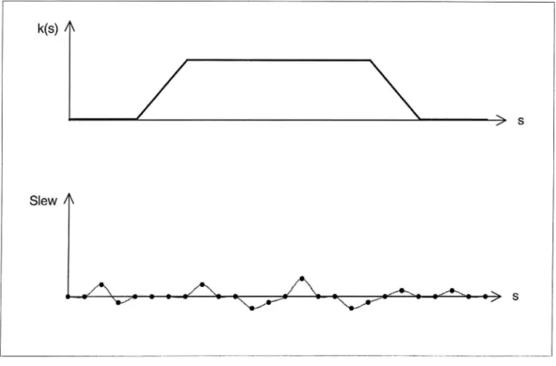
In this case, we will have full use of the analysis of curvature and slew diagrams. The calculation is assumed to create a theoretically correct alignment which reduces the misalignments but which does not include any unnecessary slew where there are no misalignments.3 Figure 4.14 shows the expected result from such a calculation.

k(s) /\

V m

Slew /\

4 W 5 S

Figure 4.14 Expected resultfrom a realignment calculation.

However, this result is normally not achieved in the first calculation. The following diagrams show a number of common patterns.

3 The objective in this chapter is not to improve the alignment, but to identify the effects in a slew diagram when changing the alignment.

(35)

k(s) A

V (D

Slew /\

Figure 4.15 Correct radius, faulty lengths of transition curves.

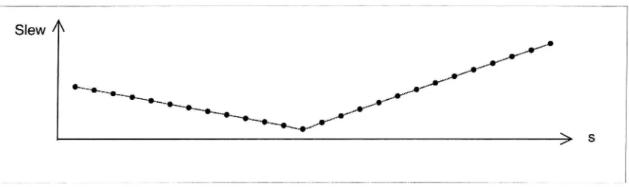
In the case of Figure 4.15, where the slew in the circular part is constant but non zero, the track engineer should not change the radius in the following calculation. The radius is correct. The slew in the circular partresults from the fact that the calculated lengths of the two transition curves are not the same as the lengths of the existing transition curves. In the next case, Figure 4.16, where the slew in the circular part changes linearly, the radius is also correct. It also seems that the length of the entering transition is correct. In order to minimise the slew, the track engineer should change the length of the run out

transition.

24 KTH TRITA FKT Report 1997:30

(36)

k(s) A

Slew 4

Figure 4.16 Correct radius, faulty length ofrun-out transition.

In Figure 4.17, the radius of the curve is not correct. This is concluded from the non linear slew in the circular part. The correct radius should be determined with the

methods discussed in Section 4.5. After a second calculation, the slew diagram will have

a basic pattern resembling one of Figures 4.14 4.16 (unless thecurve has the type of misalignment illustrated in Figures 4.11-4.12).

k(s) A V m Slew A ' a 3 f I A A... v V

Figure 4.1 7 Faulty radius.

(37)

26 KTH TRITA-FKT Report 1997:30 VTI Rapport 420A

(38)

5. Turnouts

A turnout is a device used to split one track into two. The principal parts of the turnout are the set of switches, the common crossing and the set of long sleepers, see Figure 5.1. Switches and crossings may form other combinations than a turnout, i. e. diamond crossings, single slips, but the mathematics for these types of switches and crossings work are of the same type as for a turnout.

Stock rail joint Heel of the turnout

Toe Set of switches

/

Common crossing X

Long sleepers

Figure 5.1 Principalparts ofa turnout.

There are two different types of switches. In order to avoid a thin tip, older switches have a secant geometry. In mathematical terms, this means that the branch line starts with a kink Al/f. The tip of the switch also has a specially planed geometry.

(39)

More modern switch designs have a tangent geometry and in order to avoid extremely thin switch tips, planing is essential, see Figure 5.2. This planing of the tangent geometry (and secant geometry) introduces a small lateral misalignment, which will be neglected in this document.

_ ..~ Hn' _= -: - ---.-u_{u u - n . y c - u u} u.'w-._ ---.. --u_ / / A P / /

Toe of the switch

Planing

Figure 5.2 Secant geometry and tangent geometry ofswitches.

The common crossing of a turnout may form a straight branch line or a curved one. The most common type of turnout has one or more circles in the branch line to connect the pair of switches to the common crossing. Modern turnouts may include transition curves. The tangent of the angle between the tracks at the end of the common crossing (heel of the turnout) is called the turnout angle.

(40)

The rails after the common crossing normally have such lengths that the distance between the through track and the branch line is approximately 1.75 m in order to make the turnout as short as possible. (The track spacing should not be smaller since it must be possible to insert the bolts in the fishplates at the joints of the rails.) With such small track spacings it is impossible to use single sleepers with an area large enough to carry the traffic loads. Behind the heel of the turnout there is usually a set of long sleepers which carry the four rails from the through track and the diverging track. Such sleepers are used until the track distance has increased to approximately 2.4 m. When these long sleepers are made of concrete, the standard geometry in the diverging track consists of a straight line or a curve with the same curvature function as in the common crossing. If another horizontal geometry is used, the longitudinal position of each sleeper must be adjusted since each sleeper has its specific track spacing.

Using the small angle approximation, the y coordinates for the through track yts and the branch line ybs in a straight turnout may be expressed as

yrs (S) z kts (S)dsds = HOdeS i [5.1]

mm z [Ikb.(s)dsds

[5.2]

where the function kbs(s) normally has a constant value, but may change continuously in

modern turnouts and may have an infinite value at the toe of an old type of turnout (with a switch having secant geometry).

If the turnout is placed on a curve where the through track has the curvature ktc(s), the y coordinates for the through track ytc and the branch line ybc may be written as

Ms) z [j ktc(s)dsds

[5.3]

ybc<s>z Hkbxsmsds

[5.4]

If the cant is zero, the sleepers define the track distance to be the same in the curved turnout as in the straight turnout, which may be expressed as

ybs(S)_yts(S)zybc(S)_ytc(S)

(Formula [5 .5] introduces a new approximation since it does not regard the longitudinal shifts of sleeper positions. These longitudinal shifts are not made in the same way by all railway companies. For example, the Swiss Federal Railways, SBB, apply other rules than the German Federal Railways, DB.)

The second derivative of [5.5] gives the formula of superposition4

kbc (s) z kbs (S) + km (S) [5.6]

4 The approximation [5.6] was derived for a special case (turnout with a circular branch curve, placed on a circular main line and bent according to the German rules for longitudinal sleeper shifts) by B'aseler (1931).

(41)

which may be used to approximately describe the curvature in the branch line kbc in an arbitrarily curved turnout. Expression [5.6] is accurate enough to calculate the cant deficiency inside a curved turnout, but should not be used to calculate the exact position in the x-y plane.

The turnout angle is dependent on the lengths (track spacings) and the longitudinal positions of the two last sleepers in the turnout. Even though different railway companies have different rules forthe longitudinal shifts of the sleepers, these shifts are made so that the turnout angle is unaffected by the bending of the turnout.

Formula [5.6] may be used not only to determine the curvature within a curved turnout,

but also to determine a feasible curvature pattern in an entire crossover between two parallel through tracks on curves, see Figure 5.3.

MSW?

/

/ \ / \ \ / \ /

Crossover on straight lines Crossover on curves

Figure 5.3 Curvature of crossovers placed on straight lines and on curves respectively.

(42)

6. Maintenance with lining and levelling machines

Because of imperfections in the underground and dynamic traffic load, the track geometry deteriorates non-uniformly. The reduction of track irregularities is an important part of track maintenance. This work is carried out by lining (adjustment of the lateral position of the track) and levelling machines (adjustment of the vertical position of the track). Since these machines also tamp the ballast under the sleepers, they are also called tamping machines. Since some alignments are occasionally blamed for being difficult to maintain, it is important to understand the mathematics involved in the lining and levelling operations.

There are two principal measuring systems for a lining machine; three-point lining system andfour-point lining system. (Levelling is performed With a three-point system.) When these systems are used without external orientation (i.e. calculated slew and/or lift values) the machine is working in automatic mode. If slew (and/or lift) values are used to orient the machine, it is working in design made.

x

A Working direction

b

b V

Figure 6.1 T[tree-point lining system on a straight line and on a circular

curve.

The three point system, Figure 6.1, is very simple. The track is measured at three points

A, B, C and, on straight track sections, the track at the midpoint B is slewed to a position

8 onthe straight line through the adjacent measuring points A, C. In the automatic mode, the performance of the machine is dependent on the wavelengths of the track irregularities and on the geometry of the alignment machine, which may be shown in

transfer functions (Esveld 1989). On circular curves, the track should not be slewed to

KTH TRITA FKT Report 199730

31

(43)

the point B: but to a point B where the versine [7 (distance between B and B is dependent on the radius. If the small angle approximation is used (in a local coordinate system), the versine may be expressed as

~(a+c)2 (c a)2)_a-c

~ 8-R

8-R

_2-R

[6.1]

At tangent points and within transition curves, the magnitude of the versine changes continuously. As long as the transition curve has a standardised curvature pattern, normalised versines may be calculated in advance and these normalised versines should be multiplied by a factor dependent on the change in curvature between the two adjacent elements, and distributed over the length of the transition curve. Nowadays, many lining machines are equipped with microcomputers to handle the equations involved. With the correct versines, the transfer functions will be the same on curves as on straight lines. If higher performance is required, the machine should be used in the design mode. In this case, the lateral position of measuring point A is shifted laterally according to the precalculated slew value. The smoothing of the automatic mode system is still applied and reduces the in uence of surveying errors.

X Working direction

>

a w. _ v Actual track \ - H Extrapolated ~~~~..~.circu|ar curve R > V

Figure 6.2 Four-point lining system on a circular curve and at a tangent point.

In the four-point lining system, Figure 6.2, the track is measured at four points A, B, C,

D. The measuring points A, C and D are used to determine the radius in the track. With this knowledge, the lining machine automatically feeds in the corresponding versine to measuring point B where the track is slewed. This procedure gives correct results only when all the four measuring points are placed in a straight line or when all the points are

32 KTH TRITA FKT Report 1997:30

(44)

located on a circular curve. When a tangent point T is located within the measuring base A D or when all the measuring points are placed in a transition curve, some kind of

correction values (distance between A and A ) must be fed into the measuring system.

As with the three point system, these correction values may be calculated by using a set of normalised correction values.

The arrangement of cant is based on a damped pendulum, which measures the cant. The deviation of the pendulum should be constant where the cant is constant, and should change continuously in the superelevation ramps. Neither the mathematical form of a ramp (constant gradient or S-shaped) nor the magnitude of the cant gradient has any importance for the maintenance operations, since actual cant is compared with the designed cant cross section by cross section.

It should be obvious that alignments difficult to maintain are those with very short elements, where more than one tangent point is located between the first and the last measuring points (Kufver 1990), at least when the lining machine is not equipped with a microcomputer. In this case, the correction values in three-point and four-point lining systems will not follow the standard patterns.

(45)

34 KTH TRITA FKT Report 1997:30 VTI Rapport 420A

(46)

PART II PRELIMINARY COMPARATIVE STUDIES

7. Comparisons of clothoid - circle - clothoid combinations

As shown in Chapters 3 and 4, the lateral position of the track is in uenced both by the radii and lengths of transition curves. The consequences will be investigated further in this chapter.

Figure 7.1 illustrates a curve in the x-y plane. In order to simplify the discussion, the following assumptions will be made: The lateral position and the directions of the straight lines E1 and E5 are fixed. There is only one circular part E3 in the alignment and

the two transition curves E2 and E4 have the same lengths. On these assumptions, the

curve geometry can be defined with two variables, and in this case it is reasonable to use the radius R and the length of a transition curve Lt.

Figure 7.1 Clothoid - circle - clothoid combination in the x-y plane.

In reality, it may be possible to create compound curves, to have different transition lengths and to alter the positions and directions of the adjacent straight lines. But sooner or later in the design process, the straight lines will be fixed, and normally compound curves are neither desired nor necessary. The element combination and the assumptions made in this discussion correSpond to the most frequent case in a design process.

Figure 7.1 also illustrates a number of obstacles along the railway, three catenary masts

01, 02, 03 and one turnout 04. The three masts define three lateral obstacles and the

turnout defines a longitudinal obstacle, since a turnout should preferably be located on a straight line.

(47)

Figure 7.2 A double slip as a-(binding) longitudinal obstacle in the up line of the Nyna's Line, Alvsjo'.

Figure 7.3 The parsonage as a lateral obstaclefor the Svealand Line, Eskilstuna.

(48)

The objective should now be to choose the best5 combination of radius R and lengths of the transition curves Lt. These two variables define the axes in the parametric representation in Figure 7.4. Some conditions are shown in the R Lt plane. The diagonal through the origo defines the transition length where the length of the remaining circular part is zero. The R-axis defines the zero lengths of the transition curves. The length chosen for the transition curves must be within the sector defined by these two border lines. In Figure 7.4, also inequalities, which are defined by the obstacles, are illustrated. In reality, there is at least one binding constraint (otherwise there would be no curve at all). In Figure 7.4, the obstacle 01 is never binding and may be disregarded in the analysis. It should be noted that it is necessary to make distinctions between obstacles and fixed points, since the obstacles normally define inequalities.

500 Lcircle = O _ ObStaCIG 2 \

\

Obstacle 3 300 -A / . E _\ _\ I \ Obstacle 1 .4 200 Obstacle 4 100 -\ -\ O l l l l \ 0 500 1 000 1 500 2000 2500 R (m) Figure 7.4 Curve design in the R-Ltplane.

The equation for the obstacle in the midpoint of the curve 02 and an approximate equation for the longitudinal obstacle04 may be derived from equations given in Baluch

(1983).

For the midpoint condition, the equation for comparing alignment alternatives may be expressed as

(R1+W1)

(R2 +W2)

_{[7_1]}

( l R (Ml R2

COS 2 COS 2

5 Possible object functions are discussed in Kufver (1997aand 1997b).

(49)

where Al//= the angle between the adjacent straight lines

R,- = radius in alternative i W, = lateral shift for alternative i

and for the endpoint condition, an approximate equation may be expressed as

'Ay/ Lil Aw L12

(R1+w1)-tan_2*+7z(R2+w2)-tan7+7 [7.2]

where Lt,- = length of the transition curve in alternative i

In order to systematise comparisons, slew diagrams will be used. In Figure 7.5, comparisons of five different alignments are made. As a basis for the comparison, there

is a curve combination with short transition curves A0 (rather than surveyed track, which

formed the basis for comparisons in Chapter 4). The curve combination A1 has the same

radius as A0, but longertransition curves. Since A1 is always on the inside of A0, a

comparison is not relevant. If the lateral position of A1 is acceptable, the curve combination A0 with the short transition curves can be improved by a larger radius. The

alignments should have the same lateral positions in at least one cross-section, defined

by the obstacles, as the alignment combinations Az-A4 which have the same lengths of the transition curves as A1 but slightly smaller radii.6

k(S)

Slew /b

> s

Figure 7.5 Comparisons in the slew diagram.

6 The alterations of the alignments in Figure 7.5 consist of combinations of the alterations presented in Figure 4.15 and Figure 4.17.

(50)

If the binding obstacle is placed in the midpoint of the curve, as 02 in Figure 7.1, a

comparison between A2 and A0 is relevant. If the binding obstacle is a longitudinal one

(04 in Figure 7.1) a comparison between A4 and A0 is relevant, and if the binding obstacle is placed as 03 in Figure 7.1, a comparison between A3 and A0 is relevant.

From Figure 7.5, it may be concluded that the obstacles 02 and 04 represent two

extremes. An obstacle in the midpoint of the curve requires the smallest radius compensation when changing the lengths of the transition curves. The compensation is necessary due to the change in lateral shift of the transition curve, w. A longitudinal obstacle requires the largest radius compensation when changing the lengths of the transition curves. The compensation is necessary due to the corresponding shortenings of adjacent elements.

Some numerical examples of the relations are given in Table 7.1 and Table 7.2.

Angle between Lt=l40 m Lt=180 m Lt=220 m Lt=260 m

adjacent straight lines

0.2 rad R=1947.168 m R=1888 m R=1807.860 m R=1699.424 m

0.4 rad R=1902.333 m R=1888 m R=1869.767 m R=1847.390 m

Table 7.1 Some combinations ofR and Lt which pass through the same midpoint.

Angle between Lt=140 m Lt=180 m Lt=220 m Lt=260 m

adjacent straight lines

0.2 rad R=2087.6l6 m R=1888 m R=1688.276 m R=l488.4l9 m

0.4 rad R=l986.948 m R=1888 m R=l788.960 m R=1689.816 m

Table 7.2 Some combinations ofR and Lt which fulfil the same endpoint condition.

When calculating the optimal length of a transition curve, we may expect the solution to depend on the angle between adjacent straight lines as well as the position of the binding obstacle.

In the discussion in this chapter, the obstacles have been regarded as distinct and uniquely defined, which might correspond to realignments of existing lines or new alignments in urban areas. If the curve is arranged to avoid a hill in a rural area, the obstacle may not be uniquely defined, and hence the restriction in the R-Lt plane will not be represented by a distinct curve but rather a grey shaded zone. However, the same kind of analysis should be applied, even though the distinction between permissible and non-permissible alignments may be slightly diffuse (if the restriction in question is binding).

(51)

40

KTH TRITA FKT Report 1997230 VTI Rapport 420A

(52)

8. Comparisons of different types of transition curves

8.1 General considerations

The main purpose of inserting transition curves in the alignment is to achieve a

continuous curvature function. In the literature (Alias 1984, Bloss 1936, Broman 1982, D. L. Cope 1993a, Herbst et a1 1987, Herbst, Rickert & Schiitte 1989, Gubar 1990, Gurr

1988, Kerkapoly & Lengyel 1985, Kohler 1981, Kruse 1984, Mieloszyk & Koc 1991,

Petersen 1932, Ruch 1903, Schramm 1931, 1934, 1936, 1937, 1963, 1975, Schuhr 1985,

Vojacec 1868, Zeuge 1975) there is a discussion that also the first (and sometimes also

the second) derivative of the curvature (and/or cant7) should be a continuous function.

These derivatives are correlated to the jerk and its derivatives in the vehicle body, even though these relations are of a complex nature according to the non linear mass/spring/damper system which constitutes the interaction between the track and the vehicle. In this chapter, a number of different types of transition curves, which create continuous derivatives of curvature in the alignment chain, will be presented and compared. Sometimes, these types of transition curves are justified because they are believed to be longer than the clothoid (Schuhr 1984, Weigend 1975).

The disadvantages of transition curves have already been described in Chapter 7. When lateral obstacles are present along the curve, the lateral shift requires a reduction in the radius. When longitudinal obstacles are present in the adjacent elements, a limit of the shortenings of these elements may be required.

Baluch (Rail International report from IRCA/UIC Congress 1985) criticised transition curves with continuous first derivatives since the first derivatives of cant and curvature are larger than in the clothoid type. However, it was not stated how this comparison was

made. Kohler (1981), Weigend (1987) and Weigend (1988) compared the first

derivative of cant (and hence indirectly the first derivative of curvature) for some types

of transition curves with the same lateral shift, while Herbst, Rickert & Schijtte (1989)

and Gubar (1990) compared the derivatives of curvature for different types of transition

curves with the same lengths. However, Schramm (1934, 1936, 1937, 1975) had already

observed that the cost of improvements in the second derivative (of cant) is a higher first derivative, although he meant that this price was worth paying. In this report, the comparison of different types of transition curves will be based on both the magnitudes

of the first, second and sometimes third derivatives of curvature, which will be

calculated and related to both the corresponding lateral shifts and shortenings of the adjacent elements.

Sometimes, other types of considerations could be found. Schramm (1942) noted that the discontinuities in the cant gradient in the ends of linear superelevation ramps cannot be arranged. However, in his View the smoothed ends are no longer than 5 metres and hence too short to create good train riding. Alias (1984) stated that it is impossible to arrange and accept the kinks in the cant gradient. The kinks are avoided by an empirical introduction of doucines without mathematical definition.

7 Generally, the superelevation ramp and the transition curve are assumed to coincide, and the function of cant is assumed to be of the same type as the curvature function.

Mathematical description of railway alignments and some preliminary comparative studies

Mathematical description

of railway alignments and some

preliminary comparative studies

ij'rn Kufver

h

6)

Fl

<

9..

N

L-c

a.

a.

as

*

Swedish National Road and

VTI rapport 420A - 1997

Mathematical description of railway alignments and some

preliminary comparative studies

ij'rn Kufver

Swedish National Road and

TABLE OF CONTENTS

References

69

Summary

PART I INTRODUCTION

1. Background

2. Definitions

3. Differential equations for the direction w and the

coordinates x and y

3.1 General expressions and equations for straight lines and circular

curves

mm) = Jolt/1: jk(s)ds

[3.1]

{X(S), Y(S)}

x(s) = J. cos w(s)ds = JcosJ k(s)ds ds

[3.2]

u =1/20

[3.6]

x(0) = x0

[3.10]

y(0)= yo

[311]

x = x0 + I: - (sin(w0 + k - s) Sin(l//0

[3.13]

y 2 yo + E - (COS(l//0) cos(l//0 + k - S»

[314]

l//(s) =[kds =w0+k-S

[3.15]

k (s) :1 ds

[3.18]

3.3 Equations for the clothoid

[A2] = Lt - R

[3.20]

k1 k0

w(s)=[k(s)ds=[[k0+Ejds=w0+k0s+2i42

[3.22]

yzEQ.L(2)+kO.LO.Ll+_2l.L%

[3.26]

Lt2

Lt

ALO 2 L0 LCD z 3

[3.31]

Lt

AL1 = L1 .Lc1 z 7

[3.32]

k0

2

k0

2 U3

Liz

k

=-k

k

L12

L12

have the same sign and the absolute value of k1 is less than the absolute value of kg, or if

wz1.k1"k0

[335]

₆₉

_[314]

_[3.26]

_[335]

₂

_k

_{[7_1]}