COLLISION PREDICTION MODELS WITH LONGITUDINAL DATA: AN
ANALYSIS OF CONTRIBUTING FACTORS IN COLLISION
FREQUENCY IN ROAD SEGMENTS IN PORTUGAL
Jocilene Otilia da Costa
Academic Centre of Agreste Region - University Federal of Pernambuco Road BR-104, Km 59, s/n - Nova Caruaru, 55002-970, Caruaru - Pernambuco, Brazil
Phone: + 55 84 99866 9319 E-mail: jocilene.mt@gmail.com
Elisabete Fraga Freitas, Territory, Environment and Research Centre (C-TAC) - University of Minho; Maria Alice Prudêncio Jacques, Departement of Civil and Environmental Engineering, University of Brasilia, Brazil; Paulo António Alves Pereira, Territory, Environment and Research Centre (C-TAC) - University of Minho.
ABSTRACT
In spite of the strategic importance of the national Portuguese road network, there are no recent studies concerned with either the identification of contributory factors to road collisions or collision prediction models (CPMs) for this type of roadway. This study presents an initial contribution to this problem by focusing on the national roads NR-14, NR-101 and NR-206, which are located in Portugal’s northern region. This study analyzed the collisions frequencies, average annual daily traffic (AADT) and geometric characteristics of 88 two-lane road segments through the analysis of the impact of different database structures in time and space. The selected segments were 200-m-long and did not cross through urbanized areas. Data regarding the annual traffic collision frequency and the AADT were available from 1999 to 2010. The GEE procedure was applied to ten distinctive databases formed by grouping the original data in time and space.
The results show that the different observations within each road segment present mostly an exchangeable correlation structure type. This paper also analyses the impact of the sample size on the model’s capability of identifying the contributing factors to collision frequencies, therefore must work with segments homogeneous greatest possible. The major contributing factors identified for the two-lane highways studied were the traffic volume (AADT), two-lane width, horizontal sinuosity, vertical sinuosity, density of access points, and density of pedestrian crossings. Acceptable CPM was identified for the highways considered, which estimated the total number of collisions for 400-m-long segments for a cumulative period of six years.
1. INTRODUCTION
The increasing number of collisions in rural has created the need to develop strategies to help highway agencies reducing these events. The World Health Organization revealed that more than 1.2 million people die and 50 million people are injured on the world’s roads every year, and in Portugal, these figures for 2011 were 689 and 42,162, respectively, for a country with a population of 10.5 million (WHO, 2013).
Properly registered and analyzed road collision data allows for the identification of the areas or sites where safety measures have a greater potential for success and effectiveness (Lord and Mannering, 2010). Therefore, collisions prediction models (CPMs) are important tools in promoting traffic safety in different roadway facilities. They can provide accurate estimates for the total collision frequency for a location per unit of time, which is usually a function of the roadway’s traffic and geometric characteristics. However, the interpretation of a CPM coefficient as the true effect of an incremental change in an associated roadway feature is not usually satisfactory (Hauer, 2004). According to the referenced authors, this situation can arise due to problems such as (i) the cause-effect assumed between some roadway characteristics and collisions may be not always true; (ii) the presence of a strong correlation among the model’s independent variables; and (iii) the lack of important explanatory variables in the model, which causes the coefficient of one or more variables in the model to represent the unavailable variable rather than their own effect.
The development of CPMs is based on discrete, nonnegative, and over dispersed data. Additionally, in some cases, the available data may present temporal or spatial correlations, which impose specific statistical considerations for the model development (Wang and Abdel-Aty, 2006). A comprehensive analysis of the data and the methodological issues regarding the development of analytic approaches to study the factors related to road collisions can be found in the works of (Lord and Mannering, 2010) and (Mannering and Bhat, 2014). Additionally, some modeling difficulties imposed by databases with many records of zero collisions have caused the usage of different statistical modeling approaches for CPM development, which are not easy to justify from a traffic engineering perspective (Lord et al., 2005). When the use of these approaches cannot be justified and the database is formed by temporal and/or space-related data, it is possible to develop the CPM based on aggregated number of collision observation through some time period or given space. However, the impact of this aggregation on the identification of the significant explanatory variables to the observed collision frequency need to be further investigated.
Due to the intrinsic characteristics of collision data, CPMs are commonly developed using the Poisson and negative binomial regression models (Kumara and Chin, 2003; Hauer, 2004; Caliendo et al., 2007; Anastasopoulos et al., 2012; Castro et al., 2012; Bhat et al., 2014). The form of the CPM usually consists of the product of the exposure measures’ powers multiplied by an exponential term related to the other explanatory variables. Models containing additive terms have also been referred to in the literature, where the additive component aims to account for the influence of hazard points (Hauer, 2004; Caliendo et al., 2007). Therefore, Lord and Mannering (2010) and Mannering and Bhat (2014) present an analysis of different methodological alternatives which can be used in the development of CPMs, while also point out the potentialities and limitations of each approach according with the characteristics of the available database.
An important issue related to the model’s parameters is whether one can assume that the parameters vary across observations. For the purpose of collision frequency modeling, it is usually assumed that they are constant from year to year, as referred to by Anastasopoulos and Mannering (2009) in a study regarding a comparative analysis between fixed-parameters and random parameters models (the
intercept or others parameters varies across years). They indicate some advantages of the latter models specially for applications as before-and-after studies and traffic collision trend analysis and also to incorporate the effects of the variables in models not recorded. Other papers on investigating random-parameters models can be found in the literature (Anastasopoulos et al., 2012; El-Basyouny and Sayed, 2009; Venkataraman et al., 2013). Although this modeling approach is promising, for the purpose of the present paper, the parameters constants from year to year will be considered in the models.
The collision records can be grouped by taking into account the period of the observation (usually, but not necessarily, the year) or clustered according to some spatial or other characteristics observed at a specific time period (Wang and Abdel-Aty, 2006). The observation within these groups may or may not be statistically independent from each other, but the groups are independent among themselves. The existence and type of correlation within the groups of data that form the entire database is extremely relevant when determining the complexity of the parameters’ estimation using different model types.
When the data within groups are not correlated, the basic GLM can be applied by considering the inclusion of dummy variables for time (or space) in the model. For the case of longitudinal data, the procedures for estimating the parameters are derived from the GLM procedure. For non-Gaussian outcomes, the procedures may be separated into a marginal model family, which are the generalized estimating equations (GEE), as one example, and a random-effects family, a generalized linear mixed model (GLMM) that is a more complex family of models. The latter procedure will not be considered in the present work.
The GEE procedure was developed by (Liang and Zeger, 1986) as an extension of the GLM for the analysis of longitudinal data when the primary focus of the analysis is the dependence on the model’s response to the explanatory variables. The GEE can be applied for both Gaussian and non-Gaussian response variables and is a general method for analyzing clustered data where the following are true (Wang and Abdel-Aty, 2006): (i) observations within a cluster may be correlated; (ii) observations in separate clusters are independent; (iii) a monotone transformation of the expectation is linearly related to the explanatory variables; and (iv) the variance is a function of the expectation. Regarding the correlation among the observations in a given cluster, the GEE allows for different choices including the non-correlation condition. Furthermore, different studies worked the modeling of the road safety with the GEE (Lord and Persaud, 2000; Wang and Abdel-Aty, 2006; Lord and Mahlawat, 2009; Mohammadi et al., 2014).
The main objective of this study is to identify the factors that contribute to fatal and injury collision frequency for road segments, through of the analysis the impact of different database structures in time and space. These segments are located on the Portuguese national roads NR-14, NR-101 and NR-206, which are located in Portugal’s northern region.
The type of correlation within the data related to each road segment will also be evaluated using the generalized estimating equations procedure (GEE) for modeling the longitudinal data. It is expected that the identification of the correlation type (other than the “independent” correlation) may call other modelers’ attention for the fact that this data characteristic must be evaluated in advance to the selection of the method to estimate the coefficients of CPMs.
The importance of studying collisions to improve road safety in the Portuguese northern national road system is justified by the fact that these roads serve a high concentration of cities and industrial zones. Despite its importance, recent studies concerning the promotion of road safety in those roads are
scarce. Among these studies, the work of (Gomes and Cardoso, 2012) must be highlighted. These authors studied the impact of low-cost engineering measures on the decrease of accidentalness in some stretches of a multilane national road, the NR-6. As for the identification of contributory factors for road collisions in Portuguese road system, the main focus of recent studies made in the country has been on the elements of urban roads (Couto and Ferreira, 2011; Gomes, 2013).
2.
DATA
The initial traffic collision database includes the number of fatal and injury collisions, volume and geometric characteristics data on two-lane 200-m-long highway road segments belonging to sections of highways located in northern Portugal. The data are available for the years 1999 to 2010 and these data were extracted from the database of the National Authority for Road Safety, ANSR (Autoridade
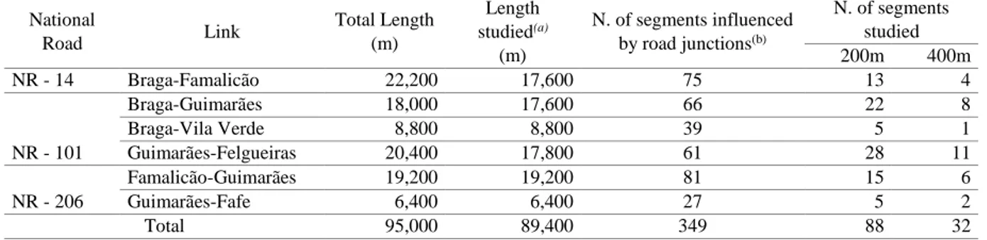
Nacional de Segurança Rodoviária). The highways and respective links are presented in Table 1. Table 1: Road 200-m-long Segments Considered for the CPMs Development
National Road Link Total Length (m) Length studied(a) (m) N. of segments influenced by road junctions(b) N. of segments studied 200m 400m NR - 14 Braga-Famalicão 22,200 17,600 75 13 4 NR - 101 Braga-Guimarães 18,000 17,600 66 22 8 Braga-Vila Verde 8,800 8,800 39 5 1 Guimarães-Felgueiras 20,400 17,800 61 28 11 NR - 206 Famalicão-Guimarães 19,200 19,200 81 15 6 Guimarães-Fafe 6,400 6,400 27 5 2 Total 95,000 89,400 349 88 32
(a) Considers only two-lane extensions not located within urban areas.
(b) 200-m-length segments presenting road junctions or containing part of a given road junction approach.
In Portugal, according to the ANSR, the analysis of critical safety points for two-lane highways must be based on 200-m-long road segments (ANSR, 2013).Therefore, the links considered were divided into 200-m-long fixed segments for which the geometric characteristics, traffic flow (expressed in average annual daily traffic) and number of collisions from the years 1999 to 2010 were registered. Some segments of these links were not included in the sample studied because they present one or more characteristics that do not fit the purpose of this study. These characteristics are the following: (i) more than two lanes; (ii) cross through urbanized areas; and (iii) contain road junctions or portions of junction approaches (with roadways for accessing cities or with interchanges for the national expressway system). Because of these criteria, only eighty-eight 200-m-long segments are present in the initial (more disaggregated) database, as shown in Table 1. To study alternative spatial variations on collision data collection reference (by means of defining different lengths for the segments considered), the original 200-m-long segments were grouped into consecutive units of 2 segments, which formed 400-m-long.
2.1. Geometric Characteristics
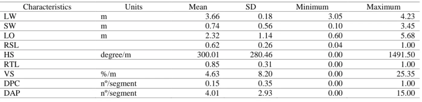
For the purpose of this study, the following geometric characteristics of each segment were considered: (i) Lane width (LW); (ii) Shoulder width (SW); (iii) Lateral offset (LO); (iv) Rate of the length in horizontal tangent per total segment length (RSL) calculated by dividing the length of straight line (tangent in horizontal alignment) by the length of the segment in horizontal projection considered (200m or 400m); (v) Horizontal sinuosity (HS), calculated by dividing the road alignment curvature at the horizontal curve (in degrees) by the length of the segment in horizontal projection considered (200m or 400m); (vi) Rate of the length in vertical tangent per total segment length (RTL) calculated by dividing by the length of straight line (tangent in vertical alignment) and SL is the length
of the segment in horizontal projection considered (200m or 400m); (vii) Vertical sinuosity (VS), calculated by dividing algebraic difference in grades (in percentage) observed at the sag or crest vertical curve by the length of the segment in horizontal projection considered (200m or 400m); (viii) Density of pedestrian crossings (DPC), which is defined as the number of pedestrian crossing facilities per length of the segment (200m or 400m); and (ix) Density of access point (DAP), which is calculated as the number of accesses to private properties (and/or to secondary roadways without exits) per length of the segment (200m or 400m).
The geometric data were collected in the field, and some statistics related to the observed values for the 200-m-long segments are presented in Table 2. It is important to highlight that these characteristics were treated as initial explanatory variables for the observed collision frequency for each road segment.
Table 2: Descriptive Statistics of the Segments’ Geometric Characteristics
Characteristics Units Mean SD Minimum Maximum
LW m 3.66 0.18 3.05 4.23 SW m 0.74 0.56 0.10 3.45 LO m 2.32 1.14 0.60 5.68 RSL 0.62 0.26 0.04 1.00 HS degree/m 300.01 280.46 0.00 1491.50 RTL 0.85 0.31 0.00 1.00 VS %/m 4.63 8.20 0.00 25.35 DPC nº/segment 0.15 0.35 0.00 1.00 DAP nº/segment 4.01 2.93 0.00 15.00
2.2. Traffic Data
The average annual daily traffic (AADT) close to the road segments is an essential indicator for the collision risk and, therefore, its presence is mandatory in prediction models. In Portugal, Estradas de Portugal - EP (Roads of Portugal) is responsible for the gathering of traffic data in the road network. Therefore considering the period in study comprises the years 1999 to 2010, there was a need to get a historic series from the segments’ AADT for that period according to the analysis and treatment of the data made available by EP. These data was complemented by data collection in loco in some of the studied road segments. The AADT values varied from 2,165 to 32,857 vehicles, with mean and standard deviation of 12,936 and 6,323, respectively.
2.3. Collision Data
The collision data for this study were provided by the National Authority for Road Safety, ANSR (Autoridade Nacional de Segurança Rodoviária), and cover the period from 1999 to 2010. The ANSR maintains a database with information gathered from the Traffic Crash Registration Form, BEAV (Boletim Estatístico de Acidentes de Viação), which is filled out at the time of the crash. In the BEAV the crash are classified into collision, run-off-road and vehicle-pedestrian collision.
The initial database, which has 12 records for each of the eighty-eight 200-m-long segments, is formed using 1,056 records, of which 815 recorded zero collisions. That is, the database is zero inflated. Therefore, a preliminary analysis aimed at verifying whether there are plausible reasons for these zeros was performed. This analysis could indicate the convenience of using a zero-inflated regression model (zero-inflated Poisson, ZIP, or zero-inflated negative binomial, ZINB). Taking into account the total number of traffic collisions registered per 200-m-long segment during the overall analysis period (12 years), the frequency distribution of the total number of collisions per segment was determined and is presented in Table 3.
Table 3: Frequency Distribution of the Number of Collisions per Segment in 12 Years
Number of collisions 0 1 2 3 4 5 6 7 8 9 11 13
Number of 200-m-long segments 9 17 12 18 5 9 5 5 2 3 2 1
The main characteristics of the nine segments with zero collisions were analyzed against correspondent characteristics observed at the six segments presenting nine or more collisions. This analysis reveals that, based on the characteristics listed in Table 2 and on the traffic volume levels, there is no technical justification for assuming that the zero-collision segments can be treated as potentially safe segments. Therefore, it was decided not to use of a zero-inflated regression model. In this case, as recommended by (Lord et al., 2005),alternative time periods for aggregating the number of collisions were considered for modeling as a means to reduce the number of records (observations) with zero collisions, as shown in Table 4.
Table 4: Number of Zero (ZR) and Total Collision (TR) Records for Different Time Observation Periods
Segment length Type of records Time observation period (in years)
1 2 3 4 6 12 200 m ZR 815 323 175 117 56 9 TR 1,056 528 352 264 176 88 (%) of ZR 77 61 50 44 32 10 400 m ZR 233 82 42 28 11 0 TR 384 192 128 96 64 32 (%) of ZR 61 43 33 29 17 0
3. METHODOLOGY
3.1. Model Formulation
The CPM for the Portuguese two-lane highway segments was developed using the generalized estimating equations (GEE) with the negative binomial link function. Therefore, the analysis considers only models with the general expression presented in Equation 5.
Volumemt
j jxjmtmt
y
E
exp
ln , (5)Therefore, it is a fixed-parameters model type from which the GLM version is derived:
j j jmt mt mt Volume x y E ln ln , ln (6)where: E(ymt) = the expected number of collisions at segment m over time period t; Volumemt = AADT
observed at segment m over time t; xj,mt = value of explanatory variable i observed at segment m over
time t; and α, γ, βj = model parameters to be estimated.
The modeling procedure followed a backward elimination starting with the AADT and all candidate variables (presented in Table 2). The final model for each combination of segment length and time observation period, which considered the three correlation structure provided by the GEE, present only the explanatory variables that are statistically significant at 5% significance level.
The identification of the factors affecting the frequency of collisions defined by the combinations of time and space was based on the model that best fit the field data. The best model for a given combination was selected based on the conditions presented in Section 3.2.
The overall best model was selected on the CURE (cumulative residuals) plot and on the marginal R2,
because the quasi-likelihood information criterion (QIC) statistic is relevant for the correlation structure evaluation. Another important consideration for model selection was the analysis of the model parameters’ sign. The parameters’ sign must be compatible with the expectation from a traffic engineering point of view.
3.2. Model Assessment
Three elements were considered for examining the goodness-of-fit for each CPM generated: the cumulative residual test (CURE), the marginal R2 and the Akaike’s information criterion (AIC) in the
GEE, which is called the quasi-likelihood information criterion (QIC) and cross validation.
The CURE test considers the difference between the number of observed and predicted collisions (the residual) as the basic element for judging the CPM fit (Hauer, 2004). The CURE plot allows for the examination of the cumulative residuals against the variable of interest, which is the Volume,it (AADT
observed at segment i over time t) for the present study. A good fit means that the CURE plot oscillates around the zero value of the cumulative residuals. Additionally, the CURE plot presents two additional curves formed by acceptable limits for the cumulative, as described (Hauer, 2004).
One fit measure introduced by Zheng (2000) for models adjusted with GEE was R2 marginal, for
which it is necessary to calculate the predicted values for the model in order to get the R2 marginal
value and then, these values are compared to the observed values. The R2 marginal value indicates
how much the response variable variance is explained by the variability of the fitted model.
In 2001, was proposed a modification for the AIC in the GEE (Pan, 2001). The modification was developed to address a model selection problem in the GEE concerning the selection of the type of correlation among observations in a given cluster (working correlation structure). The modification involves using the quasi-likelihood constructed from the estimating equations (QIC) using the working independence model and any general working correlation structure in the GEE. To select a working correlation structure in the GEE, it is necessary to calculate the QIC for various candidate working correlation structures (independent – Ind, exchangeable – Ex and autoregressive – Ar). The correlation structure to be adopted is the structure that produces the smallest QIC.
In order to ensure that the models developed in this study represent the population (generalization) and are appropriate to the conditions they are used (portability), the theory of validation is used. In this study to validate the models the cross-validation is used as suggested by Hastie et al. (2009). It is an alternative when the ability to collect new data is limited or impractical due to factors like cost and time because the original sample is used. The software used in the study was SAS 9.3®.
4. RESULTS AND DISCUSSION
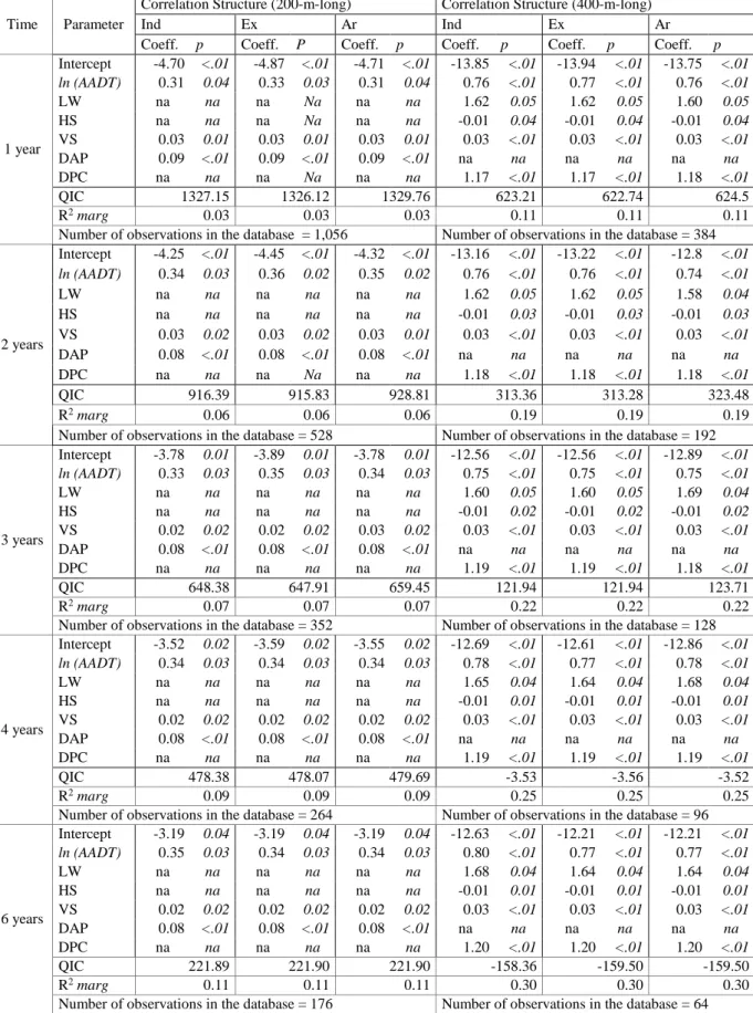
The main results for the models generated in the cases of the 200-m-long and 400-m-long segments are presented in Table 5. The AADT of grouped observations segments (2-year, 3-year, 4-6-year and year) was calculated as the arithmetic mean of the time interval considered, while collisions were summed up in this period. From Table 5, it can be observed that according to the QIC parameter, the correlation structure that best fits the longitudinal data considered is the exchangeable correlation for the first four models (1-year, 2-year, 3-year, and 4-year), according to which the correlations between any two observations within a group is constant, whereas for the latter model (6-year) the best correlation structure was the independent.
Table 5: Model Estimates for Road Segments
Time Parameter
Correlation Structure (200-m-long) Correlation Structure (400-m-long)
Ind Ex Ar Ind Ex Ar
Coeff. p Coeff. P Coeff. p Coeff. p Coeff. p Coeff. p
1 year Intercept -4.70 <.01 -4.87 <.01 -4.71 <.01 -13.85 <.01 -13.94 <.01 -13.75 <.01 ln (AADT) 0.31 0.04 0.33 0.03 0.31 0.04 0.76 <.01 0.77 <.01 0.76 <.01 LW na na na Na na na 1.62 0.05 1.62 0.05 1.60 0.05 HS na na na Na na na -0.01 0.04 -0.01 0.04 -0.01 0.04 VS 0.03 0.01 0.03 0.01 0.03 0.01 0.03 <.01 0.03 <.01 0.03 <.01 DAP 0.09 <.01 0.09 <.01 0.09 <.01 na na na na na na DPC na na na Na na na 1.17 <.01 1.17 <.01 1.18 <.01 QIC 1327.15 1326.12 1329.76 623.21 622.74 624.5 R2 marg 0.03 0.03 0.03 0.11 0.11 0.11
Number of observations in the database = 1,056 Number of observations in the database = 384
2 years Intercept -4.25 <.01 -4.45 <.01 -4.32 <.01 -13.16 <.01 -13.22 <.01 -12.8 <.01 ln (AADT) 0.34 0.03 0.36 0.02 0.35 0.02 0.76 <.01 0.76 <.01 0.74 <.01 LW na na na na na na 1.62 0.05 1.62 0.05 1.58 0.04 HS na na na na na na -0.01 0.03 -0.01 0.03 -0.01 0.03 VS 0.03 0.02 0.03 0.02 0.03 0.01 0.03 <.01 0.03 <.01 0.03 <.01 DAP 0.08 <.01 0.08 <.01 0.08 <.01 na na na na na na DPC na na na Na na na 1.18 <.01 1.18 <.01 1.18 <.01 QIC 916.39 915.83 928.81 313.36 313.28 323.48 R2 marg 0.06 0.06 0.06 0.19 0.19 0.19
Number of observations in the database = 528 Number of observations in the database = 192
3 years Intercept -3.78 0.01 -3.89 0.01 -3.78 0.01 -12.56 <.01 -12.56 <.01 -12.89 <.01 ln (AADT) 0.33 0.03 0.35 0.03 0.34 0.03 0.75 <.01 0.75 <.01 0.75 <.01 LW na na na na na na 1.60 0.05 1.60 0.05 1.69 0.04 HS na na na na na na -0.01 0.02 -0.01 0.02 -0.01 0.02 VS 0.02 0.02 0.02 0.02 0.03 0.02 0.03 <.01 0.03 <.01 0.03 <.01 DAP 0.08 <.01 0.08 <.01 0.08 <.01 na na na na na na DPC na na na na na na 1.19 <.01 1.19 <.01 1.18 <.01 QIC 648.38 647.91 659.45 121.94 121.94 123.71 R2 marg 0.07 0.07 0.07 0.22 0.22 0.22
Number of observations in the database = 352 Number of observations in the database = 128
4 years Intercept -3.52 0.02 -3.59 0.02 -3.55 0.02 -12.69 <.01 -12.61 <.01 -12.86 <.01 ln (AADT) 0.34 0.03 0.34 0.03 0.34 0.03 0.78 <.01 0.77 <.01 0.78 <.01 LW na na na na na na 1.65 0.04 1.64 0.04 1.68 0.04 HS na na na na na na -0.01 0.01 -0.01 0.01 -0.01 0.01 VS 0.02 0.02 0.02 0.02 0.02 0.02 0.03 <.01 0.03 <.01 0.03 <.01 DAP 0.08 <.01 0.08 <.01 0.08 <.01 na na na na na na DPC na na na na na na 1.19 <.01 1.19 <.01 1.19 <.01 QIC 478.38 478.07 479.69 -3.53 -3.56 -3.52 R2 marg 0.09 0.09 0.09 0.25 0.25 0.25
Number of observations in the database = 264 Number of observations in the database = 96
6 years Intercept -3.19 0.04 -3.19 0.04 -3.19 0.04 -12.63 <.01 -12.21 <.01 -12.21 <.01 ln (AADT) 0.35 0.03 0.34 0.03 0.34 0.03 0.80 <.01 0.77 <.01 0.77 <.01 LW na na na na na na 1.68 0.04 1.64 0.04 1.64 0.04 HS na na na na na na -0.01 0.01 -0.01 0.01 -0.01 0.01 VS 0.02 0.02 0.02 0.02 0.02 0.02 0.03 <.01 0.03 <.01 0.03 <.01 DAP 0.08 <.01 0.08 <.01 0.08 <.01 na na na na na na DPC na na na na na na 1.20 <.01 1.20 <.01 1.20 <.01 QIC 221.89 221.90 221.90 -158.36 -159.50 -159.50 R2 marg 0.11 0.11 0.11 0.30 0.30 0.30
Number of observations in the database = 176 Number of observations in the database = 64 na = not applicable
Table 5 shows that for the 400-m-long segments the exchangeable correlation is also found for the first four models (1-year, 2-year, 3-year, and 4-year). For the 6-year model, the results show that both the exchangeable and autoregressive correlation structures are valid. The independence correlation, which allows the longitudinal data to be treated as independent records, is only suitable for the current database for the 200-m-long segments over 6-year time period.
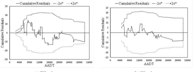
All CPMs developed are acceptable from both a statistical and traffic engineering point of view. In these models it is possible to verify that among the contributing variables studied, the major contributing factors to the collision frequency are the traffic volume, expressed in terms of annual average daily traffic (AADT), the lane width (LW), the horizontal sinuosity (HS), the vertical sinuosity (VS), the density of access points (DAP), and density of pedestrian crossings (DPC). All of these variables have a positive impact on the dependent variable (coefficients with positive sign). One important aspect to highlight is that the lane width in the database varies from 3.05 m to 4.23 m. What the results show, therefore, is that in this range, larger traffic lanes can have a negative effect on traffic safety. As a final evaluation of the previously considered acceptable models, the CURE plot for each case was developed. Figure 1 shows these plots for 200-m-long and 400-m-long segments.
(a) 200-m-long (b) 400-m-long
Figure 1: CURE Plots for the CPMs
Finally, it is necessary to ensure that the developed models represent the population (generalization) and are appropriate to the conditions they are used (portability). Therefore, in this section is showed the validation of the CPMs fitted for road segments (200-m-long and 400-m-long). The results obtained in this study are presented in terms of error models. The statistical parameter used in the analysis of the validation of these models was the root mean square error (RMSE).
The validation of CPMs was taken through the K-fold cross-validation type leave one out, since the sample size of the models allowed to leave one out cross-validation without much computational costs. Therefore, the fitted model can be considered valid if it presents error (RMSE) similar to the ones obtained by the cross-validation method.
In Table 6 are described the statistical parameters of the analysis of validation. The variation of RMSE was -1.6% to -0.8%, for 200-m-long and 400-m-long segments, respectively. Therefore, the models fitted for collisions discussed here can be considered valid, since they had small differences between the statistics of validation and adjustment. Finally, it can be concluded that the best CPM is fitted for 400-m-long segments and 6 years data aggregation.
Table 6: Statistical Parameters of the CPMs and of the Leave One Out Cross-Validation
Segment Time Means QIC Correlation
Structure R
2 mar Fitted Cross-Validation ΔRMSE
RMSE RMSE
200m 6 years 1.72 221.89 Ind 0.11 1.75 1.72 -1.6%
400m 6 years 3.58 -159.50 Ex/Ar 0.30 2.70 2.68 -0.8%
5. SUMMARY AND CONCLUSIONS
The main objective of the present study was the identification of the major contributory factors to road collision frequency for road segments of Portuguese two-lane highways located in the northern region of the country, through of the analysis the impact of different database structures in time and space. The importance of this work is to contribute to the promotion of road safety in the Portuguese northern national road system, which serves many cities and industrial zones.
The initial database considered for this study was formed by the fatal and injury collision frequency, the average annual daily traffic (AADT) and the geometric characteristics of eighty-eight 200-m-long segments during the years 1999 to 2010. This database contains 1,056 data records, of which 815 have zero annual collisions. To reduce the number of zero collision records, different databases were developed from the initial database by taking into account variations on the space and time scale of the data, as suggested by Lord et al. (2005). In terms of time, four options for aggregating the data were considered, all of which were aimed at including all of the 12-year data available. These options included 2-year groups, 3-year groups, 4-year groups, and 6-year groups. For the space scale, in addition to the 200-m-long original segments, 400-m-long segments were also considered. Therefore, including the 1-year collision data, ten different databases were analyzed.
For the studied databases of the 200-m-long road segments, the results showed that the models were able to capture the same significant contributory factors to the observed collision frequencies. These factors were the traffic volume (expressed in AADT), vertical sinuosity (VS), and density of access points (DAP). As these factors result in positive coefficients in the models, which are acceptable, when they increase, it is reasonable to expect that the collision frequency increases as well. Moreover, in the studied databases of the 400-m-long road segments, the results also showed that the models were able to capture the same significant contributory factors to the observed collision frequencies. However, these factors were the traffic volume (expressed in AADT), lane width (LW), horizontal sinuosity (HS), vertical sinuosity (VS), and density of pedestrian crossings (DPC). As these factors also result in positive coefficients in the models, which are acceptable, when they increase, it is reasonable to expect that the collision frequency increases as well.
Another important finding is that the application of the GEE procedure showed that for the road segments (200-m-long and 400-m-long), the traffic data observations (two or more) are effectively correlated; the corresponding correlation structure was the exchangeable correlation (exceptionally 6-years observations for the 200-m-long segments - correlation structure independent). So, this means that the presence and type of correlation among the observations in the database must be investigated before the development of the CPM when each location (segment or intersection) is observed over different time periods.
Regarding the validation of CPMs, with the results of cross-validation leave one out it was possible to verify that the models perform well, which is translated by low values of the statistics parameters obtained in the fit of the models and in the validation.
Finally, the study shows that the database with 400-m-long road segments and with collision data grouped for a 6-year period produces the best fitted acceptable collision prediction model according to the statistical and traffic engineering analyses, CURE plots and marginal R2, developed for the
different combinations studied. Therefore, it is observed that the different aggregations time of the collision data does not affect the contributing factors of the models, but the spatial aggregation affects. The main limitation in this study was the number of 200 meters homogenous segments included in the sample, 88, partly due to the high costs associated with the data collection and the lack of logistical resources and equipment. This sample size may have impeded the identification of the significance of some of the researched variables. Other limitation was the lack of detailed information related to all the interventions that took place in the studied NR, which didn’t allow the inclusion of other variables related to the road conditions in the models (road surface, friction coefficient, others).
Considering the promising results already obtained, it was concluded that the current study should be continued. From the databases already created, the impact of modelling with random parameters model (using GEE with trend) on the identification of contributing factors for collisions in the studied highways will be investigated, whereas this technique allows to incorporate in the model the effects of the missing variables. Studies presented in literature indicate that this type of modelling is promising and it is particularly useful for complementary analysis using CPMs such as before-and-after studies and studies aimed at identifying accentuated variations in collision frequencies in the road elements researched throughout the units of time included in the analysis’ period.
REFERENCES
Anastasopoulos, P.; Mannering, F. (2009). A note on modeling vehicle accident frequencies with random-parameters count models. Accident Analysis and Prevention, Vol. 41, pp. 153-159.
Anastasopoulos, P.; Mannering, F.; Shankar,V.; Haddock, J. (2012). A study of factors affecting highway accident rates using the random-parameters tobit model. Accident Analysis and Prevention, Vol. 45, pp. 628-633.
ANSR - National Authority for Road Safety. (2013). Road Crashes (in Portuguese). Road Safety Observatory. Lisbon, Portugal.
Bhat, C.; Born, K.; Sidharthan, R.; Bhat, P. (2014). A count data model with endogenous covariates: Formulation and application to roadway crash frequency at intersections. Analytic Methods in Accident Research, Vol. 1, pp. 53-71.
Caliendo, C.; Guida, M.; Parisi, A. (2007). A crash-prediction model for multilane roads. Accident Analysis and Prevention, Vol. 39, pp. 657-670.
Castro, M.; Paleti, R; Bhat, C. (2012). A latent variable representation of count data models to accommodate spatial and temporal dependence: Application to predicting crash frequency at intersections. Transportation Research Part B, Vol. 46, 2012, pp. 253-272.
Couto, A.; Ferreira, S. (2011). A note on modeling road accident frequency: A flexible elasticity model. Accident Analysis and Prevention, Vol. 43, pp. 2104-2111.
El-Basyouny, K.; Sayed, T. (2009). Accident prediction models with random corridor parameters, Accident Analysis and Prevention, Vol. 41, pp. 1118-1123.
Gomes, S. (2013). The influence of the infrastructure characteristics in urban road accidents occurrence. Accident Analysis and Prevention, Vol. 60, pp. 289-297.
Gomes, S.; Cardoso, J. (2012). Safety effects of low-cost engineering measures. An observational study in a Portuguese multilane road, Accident Analysis and Prevention, Vol. 48, 2012, pp. 346-352. Hastie, T.; Tibshirani, R.; Friedman, J. (2009). The Elements of Statistical Learning: Prediction, Inference and Data Mining. Springer, Verlag.
Hauer, E. (2004). Statistical Road Safety Modeling. Transportation Research Record, 1897, pp. 81-87. Kumara, S.; Chin, H. (2003). Modeling Accident Occurrence at Signalized Tee Intersections with Special Emphasis on Excess Zeros. Traffic Injury Prevention, Vol. 4, pp. 53-57.
Liang, K.; Zeger, S. (1986). Longitudinal data analysis using generalized linear models. Biometrika, Vol. 73, pp. 13-22.
Lord, D.; Mannering, F. (2010). The statistical analysis of crash-frequency data: A review and assessment of methodological alternatives. Transportation Research Part A, Vol. 44, pp. 291-305. Lord, D.; Mahlawat, M. (2009). Examining the application of aggregated and disaggregated Poisson-gamma models sub-jected to low sample mean bias. Transportation Research Record, 2136, pp. 1-10. Lord, D.; Persaud, B. (2000). Accident Prediction Models With and Without Trend – Application of the Generalized Estimating Equations Procedure. Transportation Research Record, 1717, pp. 102-108. Lord, D.; Washington, S.; Ivan, J. (2005). Poisson, Poisson-gamma and zero-inflated regression models of motor vehicle crashes: balancing statistical fit and theory, Accident Analysis and Prevention, Vol. 37, 2005, pp. 35-46.
Mannering, F.; Bhat, C. (2014). Analytic methods in accident research: Methodological frontier and future directions. Analytic Methods in Accident Research, Vol. 1, pp. 1-22.
Mohammadi, M.; Samaranayake,V.; Bham, G. (2014). Crash frequency modeling using negative binomial models: An application of generalized estimating equation to longitudinal data. Analytic Methods in Accident Research, Vol. 2, pp. 52-69.
Pan, W. (2001). Akaike’s Information Criterion in Generalized Estimating Equations. Biometrics, Vol. 57, pp. 120-125.
Venkataraman, N.; Ulfarsson, G.; Shankar, V. (2013). Random parameter models of interstate crash frequencies by severity, number of vehicles involved, collision and location type. Accident Analysis and Prevention, Vol. 59, pp. 309-318.
Wang, X.; Abdel-Aty, M. (2006). Temporal and spatial analysis of rear-end crashes at signalized intersections, Accident Analysis and Prevention, Vol. 38, pp. 1137-1150.
WHO - World Health Organization. (2013). Global status report on road safety 2013: supporting a decade of action. Geneva, World Health Organization.
Zheng, B. (2000). Summarizing the goodness of fi of generalized linear models for longitudinal data. Statistics in Medicine, Vol. 19, pp. 1265-1275.