Using k-means and PCA in construction of a stock portfolio

(1)

MASTER (1 YEAR) THESIS IN MATHEMATICS / APPLIED MATHEMATICS

Using k-means and PCA in construction of a stock portfolio

by

Alagie Malick Jeng

Magisterarbete i matematik / tillämpad matematik

DIVISION OF APPLIED MATHEMATICS

MÄLARDALEN UNIVERSITY SE-721 23 VÄSTERÅS, SWEDEN

(2)

Master (1 year) thesis in mathematics / applied mathematics

Date:

2014-06-01

Project name:

Using k-means and PCA in construction of a stock portfolio

Author(s):

Alagie Malick Jeng

Supervisor(s):

Ying Ni, Christopher Engström

Reviewer: Daniel Andrén Examiner: Sergei Silvestrov Comprising: 15 ECTS credits

(3)

Abstract

There is a various analysis that has been presented on the issues that pertain to risk when con-structing stock portfolios in the financial market. The information given by most researchers is insufficient to warrant conclusions on the issues of conditional volatility and unconditional volatility hence the need for the study. The operations that take place in the financial market often rely on the different instruments like stocks, bonds, funds, and commodities. With this paper, we are using K-mean clustering and PCA (principal component analysis) in order to try to minimize risk when constructing Stock Portfolio. Results of both methods will be evalu-ated and compared experimentally (by implementing the methods and looking at the resulting portfolio).

(4)

Acknowledgements

I thank The Almighty God for the good health and well-being that were needed for the thesis. I am very grateful to my supervisors for their endless efforts in guiding me all the way through this process. Special thanks to Ying Ni and Christopher Engström for many constructive and useful comments and proposals which guide and helped me positively to improve my thesis work. Also, my sense of gratitude to all those who directly or indirectly have lent a hand in this venture. Finally, I would like to extend my deepest gratitude to Awa Samba-Jeng, Penda Njie-Jeng and all my kids without whose love, support, and understanding I could never have completed this master’s degree.

(5)

Chapter 1 Introduction

Principal Component Analysis (PCA) is a data reduction technique used to accentuate vari-ation and display robust patterns in a data set. It is often used to make data simple in order to examine and envision. It is a simple, non-parametric technique for extracting important information from a complex data set. With little efforts, Principal Component Analysis can generate a road-map for how to reduce a large data set to a lower dimension, in order to reveal the hidden, simplified structure that often underlie it. Johnson and Wichern (1998) [12] stated that Principal Component Analysis explains the variance-covariance structure of a group of variables through a few linear combinations of these variables. It aims to transform the ob-served variables to a new set of variables which are uncorrelated and arranged in decreasing order of importance.

K-means clustering is a partitioning technique. With this technique, a cluster is represen-ted by the center of mass of their members. It is among the simplest autonomously learning techniques that solve the renowned clustering problem. The method follows an easy route to categorize a given data over a specific number of clusters. Also, calculating the center of each cluster as the centroid of its member data vector is equal to finding the minimum of the sum of square cost function by using coordinate descent method. In k-means clustering, each cluster in the partition is identified by its member’s object and by its centroid. The point to which the sum of the distance from all objects in that cluster is minimized is the centroid of each cluster. K-means clustering aims to partition n observation into k clusters in which each observation being part of the cluster with the closest mean, serving as a prototype of the cluster. It locates a partition in which objects within each cluster are as close to each other as possible. K-means clustering uses an iterative algorithm that reduces the sum of distances from each object to its clusters centroid, above all clusters. This algorithm shifts objects between the clusters to a point that is not possible for the sum to decrease further. The outcome is a set of clusters that are compact and well-divided.

A collection of stocks pursued together is called a stock portfolio, and from that portfolio, a firm or person can purchase and sell stocks in order to generate money. Portfolios are usu-ally managed by financial experts or held directly by investors. Portfolios are selected in such a way as to minimize the risk. The risk of stock portfolios depends on the proportions of the

(8)

individual stocks, their covariances, and variances. The risk of the portfolio will change if there is a change in any of these variables. When stocks are randomly selected and combined in equal proportions into a portfolio, the systematic risk of a portfolio decline as the number of different stocks in it increases.

1.1 Aims of the project

The goal of this project report is to provide the reader with a wider understanding of how both methods (the PCA and k-mean clustering) can be used, in order to minimize risk when constructing a stock portfolio. Hence, it impossible to avoid risk in investment, we then try to find ways to minimize it.

To explore the connection between these two widely used methods (k-means clustering and PCA), we will introduce mathematical concepts that are used in k-mean clustering and PCA methods. That is before getting into more details about the PCA and k-mean clustering. To realize our objective, we will use the software system XLSTATS as an implementation of PCA and k-mean clustering. Other software that could be used are MATLAB, SAS, SPSS, SPAD, STATAetc. We used the XLSTATS, since the system has the ability to contain a large amount of data, and also because of its availability. We will also try to make some generalizations re-lating to the potential gains, and pitfall of using k-means clustering and Principal Component Analysis in relation to the interpretation of our results.

(9)

Chapter 2 Literature survey

The literature survey includes publication by Richard A. Johnson and Dean W. Wichern, pro-fessors at the University of Wisconsin and Texas A and M University, respectively, namely Johnson, A.R., and Wichern, W.D. (1998). Applied multivariate analysis, 4th ed. New Jersey: Pretence-Hall, Inc.; and other articles in Dings, C., and He, X. 2004. K-means clustering via Principal Component Analysis. Pro. International Conference on Machine Learning. Banff, Canada.

We will use the theoretical perspective on the statistical methods or techniques for describ-ing and analyzdescrib-ing multivariate data in the work by Johnson and Wichern (1998), and Ddescrib-ings and He (2004). As supporting knowledge necessary for making a proper interpretation, se-lecting appropriate techniques, and understanding their strength and weaknesses. Previous research and reviews on large data analysis using either k-means clustering or Principal Com-ponent Analysis or both will be our main resources examining and evaluating various issues on the data analysis in a comparative context.

For analyzing the ever-growing massive quantity of high dimensional data, data analysis meth-ods are significant for analyzing. According to Duda et al., (2000); Hastie et al, (2001); Jain and Dubes, (1988), cluster analysis attempts to pass through the data quickly to gain first or-der comprehension. This is done by partitioning data point into disjoint groups such as data point belonging to different clusters are dissimilar. The k-means method is one of the most popular and efficient clustering methods. The method uses prototypes (centroids) to represent clusters by optimizing the squared error function Hartigan and Wang, (1979); Lloyd, (1957); MacQueen, (1967). MacQueen, (1967), suggest the term k-means for illustrating an algorithm of his that allocates each item to the cluster having the closest mean (centroid). The process is illustrated in chapter four.

Johnson and Wichern, (1998) suggested that it is desirable to rerun the algorithm with a new original partition. That is to ensure the stability of the clustering. As the clusters are resolved, intuitions regarding their interpretations are assisted by rearranging the list of items as a result that those in the first cluster occur first. Then, follow by those in the second, third, and so on and so forth. A table of the within-cluster variance and cluster mean or centroid assists to

(10)

delineate differences of the group.

The importance of single variables in clustering must be judged from a multivariate perspect-ive (Johnson, A.R., and Wichern, W.D. 1998). Multivariate observations (all the variables) decide the reassignment of items and the cluster centroids. They further mentioned the values of the descriptive statistics measuring the significance of single variables are functions of the final configuration and a number of clusters. And on the contrary, descriptive measures can be of importance in recapturing the success of the clustering process.

Johnson and Wichern (1998) emphasized on a strong argument for not fixing a number of clusters, K, in advance, including the following:

A. If two or more seed’s point, unintentionally lie in the midst of an individual cluster, resulting clusters will be badly differentiated.

B. The presence of an outlier might generate the least group with very disperse items. C. The sampling technique may be such that the data from the unusual group does not

prevail in the sample. Even if the population is known to contain K groups, forcing the data into K groups would lead to not meaningful clusters.

When a single run of the algorithm requires the user to specify K, for different alternatives, it is always good to rerun the algorithm.

According to Jollife (2002), high dimensional data are often transformed into lower dimen-sional data through the Principal Component Analysis (or singular value decomposition) where logical patterns can be noticed clearly. It is also stated that such unsupervised dimensional re-duction is used in wider areas. Given examples are information retrieval, image processing, genomic analysis, and meteorology. With reference to Zha et al., (2002), it is usual that Prin-cipal Component Analysis is the used data in a lower dimensional subspace while k-means is the applied data in the subspace. However, in other cases, Ng et al., (2001), data are rooted in a low dimensional space such as the eigenspace of the graph Laplacian, and k-means are then applied. The principal components are really the continuous solution of the cluster mem-bership indicators in the k-means clustering method (Ding and He, 2004). For example, the Principal Component Analysis dimension reduction automatically performs data clustering according to the k-means objective function. This generates a significant justification of PCA-based data reduction.

The Principal Component Analysis takes up the dimension with the largest variance, which is the main basis of PCA-based dimension reduction. Eckart and Young, (1936) mentioned that, mathematically, this is equal to finding the best low-level estimation (in L2 norm) of the

data through the SVD (singular value decomposition). Jonhson and Wichern, (1998) stated that; an analysis of principal component often discloses relationships that are not suspected before. Thus, permits an interpretation that would not normally result. They further described

(11)

the analysis of principal components as more of a means to an end rather than an end in them-selves. They often serve as middle steps in the much larger investigation. A given example is that principal components may be input to a multiple regression or cluster analysis.

Minimizing risk in the construction of stock portfolio is an important task. Since investors can generate steady returns, if the risk can be minimized in the portfolio construction. Ac-cording to S. -H. Liao et. al, (2008), there is no universal model that can predict everything well for all problems or even be a single best forecasting method for all situations. To do a stock portfolio management, different analysis methods have been applied by many research-ers, including the use of the Markowitz model (Tiwari, M. K., Nanda, S.R., and Mahanty, B. (2010)).

2.1 Previous studies

There is a conviction about stock markets like high risk and high returns. Albeit there were numeous of prospective investors, and only a very small number of them are investing in the stock market. The inability of risk taking know how of investors is the main reason be-hind it. They want to save their money if they get low returns. They do not have a proper guidance for choosing their portfolio, which is one significant for this problem [19]. Finding effectual ways to summarize and envisage the stock market data to give individuals or estab-lishments meaningful information about the market behavior for investment decisions is one of the most significant problems in modern finance. In this day and age, traders are required to use different forecasting methods rather than a single method to gain multiple signals and more information about the future of the market. Existing clustering algorithms encounters a problem in handling multidimensional data. The intrinsic scarceness of the points creates multidimensional data challenges for data analysis. Researchers have made a lot of attempts for the improvement of the performance of the k-means clustering algorithm. Generally, by applying the methods from statistics or linear algebra such as Principal Component Analysis, the dimensionality reduction is accomplished [5].

Tiwari, M.K., Nanda, S.R, and Mahanty, B. (2010) indicated that k-means build the most compact cluster as related to other techniques such as Fuzzy c-means for stock classification data. Whereby, stocks can be selected from the clusters in order to construct a portfolio, minimizing portfolio risk and related the returns to that of the benchmark index. Hierarch-ical agglomeration and recursive k-means clustering are assumed to be an effective clustering method to predict the short-term stock price trends after the publication of a financial report. According to H. Kopeti (2010), the share price moving of each individual company creates a time series graph with dissimilar patterns. To select the right to invest in, the investors require identifying and comprehend all the patterns of the share price trend and select the share with the favorable pattern.

Recent research recommends that Principal Component Analysis data reduction can help in market or data segmentation. PCA generates a way to diminish large data-sets to vital

(12)

vari-ables. To conduct segmentation analysis on this diminished data-set turns out to be more effective in many cases rather that the total dataset, since the most important problems in modern finance are finding effectual ways to summarize and envisage the stock market data to provide individuals or establishments useful information about the market behavior for in-vestment decisions. The huge amount of valuable data created by the stock market has enticed researchers to explore this problem domain using various methodologies.

(13)

Chapter 3 Mathematical Background

In order to conduct a Principal Component Analysis and k-mean clustering on a data set, many measures were taken and procedures followed. Therefore, regarding our procedures, we will manage to provide our best explanation and information as possible for the reader to under-stand. This section will provide mathematical concepts that will be required to understand the process of k-mean clustering and the process of PCA.

We now introduce the definitions to sample statistics, namely sample mean, variance/standard deviation matrix, which are unbiased estimates of the population counterpart.

3.1 Statistics

Sample mean

Sample mean refers to the sum of list numbers divided by the size of the list. For example, if we have a sample of observations of random variable A. There exists S observations for random variable A:

A₁, A2, A3, ...., AS−1, AS

The sample mean of A is given by ¯ A= A1+ A2+ A3+ .... + AS−1+ AS S = 1 S S

∑

i=1 A_i (3.1) Sample variance

Sample variance is a measure of the spread of the observation around the mean, we therefore can compute the variance by: We begin first by taking the difference between A1 and ¯A, and

square it (A1− ¯A)2. Likewise, the squared deviations of the other observation from the mean

are (A2− ¯A)2, ...., (AS− ¯A)2. The sample variance is defined as the sum of these terms, divided

by S − 1 :

Variance(A) =(A1− ¯A)

2_{+ (A}

2− ¯A)2+ ... + (AS− ¯A)2

(14)

=∑i(Ai− ¯A)

2

S− 1 (3.3)

Sample standard deviation

Sample standard deviation (s) is an alternative measure of the spread, which merely is the square root of the variance. So

s_A= s

∑i(Ai− ¯A)2

S− 1 (3.4)

The sample standard deviation shows the amount of variation or dispersion from the average that exists. A high sample standard deviation indicates that the data points are spread over a large range of values, while a low sample standard deviation indicates that the points tend to be close to the mean.

Sample covariance

Sample covariance is used to determine how two variables vary together. Thus Covariance(A, B) =∑i(Ai− ¯A)(Bi− ¯B)

S− 1 (3.5) in the event, we find that the covariance is negative, this means that B is often below it’s mean or average when A is above it’s mean or average, and vice versa. Therefore, the one variable tends to go down while the other goes up. But, if we find that the covariance is positive, this means that B is often above its mean or average when A is above its mean or average, vice versa. Therefore, the variables increase together and decreases together. If we normalize the covariance by dividing it by the square root of the product of the variances, a very significant statistic arises: SA,B= ∑i (Ai− ¯A)(Bi− ¯B) S− 1 · 1 q ∑i(Ai− ¯A)2 S−1 · ∑i(Bi− ¯B)2 S−1 (3.6) S_A,B=_p ∑i(Ai− ¯A)(Bi− ¯B) ∑i(Ai− ¯A)2· ∑i(Bi− ¯B)2 (3.7) S_A,Bis called the correlation coefficient, and one can show that −1 ≤ SAB ≤ 1

Covariance matrix

Covariance matrix is defined as a matrix whose element in the i, j position is the covariance between the ithand jthelements of a random vector. Therefore, the definition of the covariance matrix for a set of data with n dimension is:

(15)

where Cmxn is a matrix with n rows and n columns, and dimx is the xth dimension. Equation

(3.8) signifies that, if we have a n-dimensional data set, then the matrix has n rows and columns and each entry in the matrix is the result of calculating the covariance between two separate dimensions [6].

3.2 Matrix Algebra

eigenvalues or eigenvectors of a matrix Definition 3.1

If Ax = λ x where A ∈ Mnxn(K), λ ∈ K, v ∈ Mnxn(K) then λ is an eigenvalue of A and x is a

(right) eigenvector if x 6= 0. An eigenvalue with corresponding eigenvector x is an eigenpair (λ , x).

Matrices usually have multiple eigenvalues and eigenvectors, but a single eigenvalue can also be associated with multiple eigenvectors. We will get the same multiple of a vector as a res-ult if we scale the vector by some amount before we mres-ultiply it because its resres-ult to another property of eigenvectors. This happens because scaling a vector by some amount does not change its direction, but makes it longer. All the eigenvectors of a matrix are perpendicular regardless of the number of dimensions we have, and it is important since it means that we can transmit the data in an expression of these perpendicular, regardless how many dimensions you get. Instead of expressing the data in terms of y and x-axes, we can express them in terms of perpendicular eigenvectors.

Definition 3.2

Where two nxn matrices A, B are given, we say that A and B are similar if there is an invertible nxnmatrix P such that

B= P−1AP (3.9) As a result of this, similar matrices share not only eigenvalues but many properties.

Theorem 3.1

Let matrices A, B be similar, this result to A, B having the same • Rank

• Eigenvalues (but generally not the eigenvectors) • Trace

• Determinant, det(A) = det(B)

(16)

The Euclidean distance

The Euclidean distance or simply distance examines the root of squared differences between the coordinates of two objects.

d(a, b) = s n

∑

k=1 (a_k− b_k)2 _(3.10)

Where a = (a1, a2, ..., an) and b = (b1, b2, ..., bn) are two points in the Euclidean n-space.

3.3 Markowitz portfolio optimization model (1952)

Markowitz invented a model for creating an efficient portfolio. According to Markowitz’s model, the risk of a stock is the standard deviation and the return of a stock is the mean return. The portfolio that offers the greatest return for each level of risk is the efficient frontier of portfolios. A graph of the lowest possible variance that can be achieved for any given level of expected return is the minimum variance frontier. The portfolio of risky assets that has the lowest variance of all risk asset portfolios is the total minimum portfolio. The efficient frontier is also referred to as the limit of all investments that are within the minimum-variance and have higher returns than the total minimum variance portfolio. The weighted return of the stocks is the portfolio return. The expected return for a portfolio is calculated as:

E(R_ρ) =

k

∑

j=1

vjE(Rj) (3.11)

The weights in stock i and j are vjand vl, and Rjis the returns on stock j .

The variance of a portfolio containing two assets j and l is calculated as:

σ_ρ2= v2_jσ2_j + v2_lσ_l2+ 2vjvlCov(Rj, Rl) (3.12)

If σρ is the portfolio risk and k the number of underlying stocks, generalizing the equation to

accommodate more than two assets result in the equation σ_ρ2= k

∑

j=1 k

∑

l=1 v_jv_lCov(Rj, Rl) (3.13)

where the covariance between the stock price of j and l is σjl. With fixed returns, we can state

the problem of minimization of risk as: minimize

σ_ρ2= vTSv (3.14) subject to

(17)

vTR= Re (3.16) where v is valued between 0 and 1 which signifies the weight vector. S signifies the covariance matrix of stocks, the expected return is Re and the mean return of each stock (R) is defined as R_t = log( Pt

Pt−1). Where the price of the stock at time ’t’ is Pt.

Since we are working on more than two-assets portfolio, we used the matrix multiplication to determine our expected return in the the portfolio.

The expected return for the portfolio is calculated as: Re= vTR= [vj...vl]       E(Rj) . . . E(Rl)      

where: v is the vector of the weights of the individual asset and R is the vector of the expected returns of the individual assets ( j through l) in the portfolio.

The portfolio standard deviation is calculated as σρ = √ vT_Sv₌       [vj...vl]       σj j ... σjl . . . . . . σl j ... σll             v_j . . . V_l             1 2

where S is denoted as the variance-covariance matrix returns in the portfolio. The variance of the asset’s returns is the covariance of an asset’s returns with returns for the same asset (such as σjl. The definition of v remains the same as in the previous section.

The optimal weights for the asset in a portfolio are the ones that maximize the value of the Sharpe Ratio for the portfolio.

S_ρ =E(Rρ) − rf σρ

(3.17) rf= risk free rate

To find the optimal risky portfolio, we can use assets weights (wi) that maximize the Sharpe

Ratio. We know that for two risky assets, the portfolio expected return and standard deviation is given by

Re= wE(Rj) + E(Rl)(1 − w) (3.18)

σp=

q

(18)

So, we require to maximize the Sharpe Ratio

S_p= _q wE(Rj) + E(Rl)(1 − w) σ2_jw2+ δjl2w(1 − w) + σ_l2(1 − w)2

(3.20) by selecting w appropriately. By using Solver in Excel, this can also be done. The following method can also generates the weights for the optimal portfolio with only two assets:

wj=

σ_l2(E(Rj) − rf) − σjl(E(Rl) − rf

σ_l2[E(Rj) − rf] + σ2j[E(Rl) − rf] − σjl[E(Rj) − rf+ E(Rl) − rf]

(3.21) w_l = (1 − wj) (3.22)

Similarly through the use of some matrix algebra you can also find the solution for N > 2. Using Solver to solve the optimal risky portfolio weights (with N risky assets), we can use the following steps; identifying all of the risky assets to part of the whole investment, calculate returns series(from prices) for each risk free asset and the risky asset and find out the average for each of the mentioned, calculate the covariance matrix of the risky assets, insert the method for the Sharpe ration into a cell, create a column of cells for the portfolio weights, and utilize Solver to maximize the Sharpe ratio by altering the weights, under the condition that the weights are non-negative and add up to one.

Capital Allocation and Separation Property

The optimal mix of weights for assets in the risky portfolio is the mix that created a portfolio along the efficient frontier that is tangent with the Capital Allocation Line. The results in the CAL with the largest shape ratio is the optimal risky portfolio.

Separation property says that there are two independent tasks involved with the portfolio choice property. We begin by determining the optimal risky portfolio. The risky portfolio is the best regardless of the level of risk aversion of the investors. The following task is the capital allocation between the risky portfolio and the risk-free asset, which is based on the individual investor’s risk aversion and the relative rates of return for the risky portfolio and risk-free assets.

x∗= E(Rρ) − rf Bσ2

ρ

(3.23) where x∗is the proportion of the portfolio invested in the risky portfolio and B is a measure of the investor’s risk aversion.

The method we used to find our optimal weights is called solver. First, we calculated the optimal portfolio and to see whether we can do better than the results we got, we used solver to determine the optimal weights and at the same time to maximize the Sharpe Ratio.

(19)

3.3.1 Recent developments in the methods use

According to Andrews, N. O., and Fox, E. A., (2007) many recent developments have basis in hierarchical and partitional algorithms which have been the dominant clustering methods. Hierarchical algorithms function by consecutively combining stocks converging at the bot-tom of the hierarchy or tree. In this method, the number of clusters are not required to be provided beforehand, and the resulting cluster’s hierarchy is browsable, which are its advant-ages. On the other hand, partitional method, of which the k-means is the classical example, begins by selecting K initial stocks as clusters. It iteratively allocates stocks to clusters while updating the centroid of these clusters. It is usual to regularize stock’s vectors and use a co-sine similarity other than Euclidean distance. The forthcoming algorithm is called spherical k-means.

3.4 Limitations

Similar to another algorithm, both the PCA and the k-mean clustering methods have some limitations: The limits of the Principal Component Analysis branch from the fact that it is a projection method and occasionally the mental picture lead to wrong interpretation. There are some ways to avoid such pitfalls. With PCA, dimension reduction can only be achieved if the original variables were correlated. In the event that the variables were uncorrelated, PCA does nothing other than ordering the variables according to their variance. In Principal Component analysis, the directions with the largest variance are assumed to be of most interest. We only consider orthogonal rotations of the original variables, and PCA is based only on the covari-ance matrix of the data and the mean vector. Some distributions such as multivariate normal are completely characterized by this and others are not.

With k-mean clustering different partitions can result in different final clusters. To compare the result achieved, it is helpful to rerun the program using the same as well as different K values. In k-mean clustering, fixed number of clusters can make it difficult to predict what K should be. The difficulty also in comparing the quality of the clusters produced, such as different initial partitions. And it does not work well with non-globular clusters. It is also vulnerable to outliers and noise.

3.5 Methodology

In the methodology, we illustrate the procedure that was taken to collect the data for this re-port, the reason behind choosing the techniques followed in this rere-port, and the significance of each of the techniques applied in this project report.

The paper will be processed using quantitative analysis since it is deemed relevant and most adequate for such type of report. It will be based on secondary data analysis. In other words, secondary data will be studied and analyzed for the purpose of this thesis paper. And we draw

(20)

our conclusion from the collected and processed data using k-means clustering and principal component analysis. To conduct our project report, the following procedures were taken: Ini-tially, was deciding on the area of interest and topic. Since, minimizing risk in a construction of stock portfolio is a common area of interest, and is chosen as a topic for the project report. Followed by, establishing the information, research trait. The research trait was prepared to be k-means clustering, Principal Component Analysis, and Stock Portfolio used in searching secondary data from databases, such as journals, books, websites, etc. The literature review relating to the trait processed concept and conceptual framework chosen.

3.6 The data

We collected data on 85 stocks historical prices (2010-10-14 to 2014-05-02) each consisting of 899 observations from the website of Euroinvestor [7]. That is to say that there are 899 observations and 85 variables, each a time series. The variables are composed of stocks from different branches, like banking, fashion, mining, construction, etc. The variables are Aarhus-Karlshamn AB, Active Biotech AB, Addtech AB ser B, ABB Ltd, Alfa Laval AB, Assa Abloy AB ser B, AstraZeneca PLC, Atlas Copco AB ser A, Atlas Copco AB ser B, Atrium Ljun-gberg AB ser B, Avanza Bank Holding AB, Axis AB, Beijer AB G & L ser B, Beijer Alma AB ser B, Bilia AB ser A, BillerudKorsnäs AB, BioGaia AB ser B, BioInvent International AB, Björn Borg AB, Boliden AB, Bure Equity AB, Clas Ohlson AB ser B, Diös Fastigheter AB, Electrolux AB ser B, Ericsson Telefonab L M ser, Eniro AB, Fagerhult AB, Fast Partner AB, Fastighets AB Balder ser B, Fenix Outdoor AB ser B, Getinge AB ser B, Gunnebo AB, Haldex AB, Heba Fastighets AB ser B, Hennes & Mauritz AB H & M ser, HiQ International AB, Industrial & Financial Systems, Indutrade AB, Intrum Justitia AB, Investor AB ser B, JM AB, KappAhl AB, Klövern AB, Kungsleden AB, Lindab International AB, Lundin Petroleum AB, Medivir AB ser B, Modern Times Group MTG AB ser, Net Insight AB ser B, New Wave Group AB ser B, Nibe Industrier AB ser B, Nobia AB, Nolato AB ser B, Nordea Bank AB, Nordic Mines AB, Nordnet AB ser B, Proffice AB ser B, Rezidor Hotel Group AB, Sagax AB pref, SAS AB, Sandvik AB, Scania AB ser B, Securitas AB ser B, Skandinaviska En-skilda Banken, Skanska AB ser B, SKF AB ser B, SkiStar AB ser B, Ssab AB ser A, Sweco AB ser A, Sweco AB ser B, Swedbank AB ser A, Swedish Match AB, Swedol AB ser B, Svenska Cellulosa AB SCA ser, Svenska Handelsbanken ser A, Tele2 AB ser B, TeliaSon-era AB, TradeDoubler AB, Transcom WorldWide S.A SDB ser A, Transcom WorldWide S.A SDB ser B, Unibet Group PLC, Wallenstam AB ser B, Wihlborgs Fastigheter AB, Volvo AB ser B, and Öresund Investment AB. An observation is the value at a specific time, of a specific variable. We compute the logarithmic daily returns for each stock using formula log( pt

pt−1) ,

where the price of the stock at time ’t’ is pt as described earlier (in sec 3.3). Thus, obtain 899

daily returns for each stock under consideration. We used the log returns of the stock prices because stock returns are not precisely normal.

We will use the book Applied Multivariate Statistical Analysis [12] and articles pertaining to k-means clustering, Principal Component Analysis and stock portfolios. To ascertain the effect of risk minimization in the construction of the stock portfolio, data retrieved from the

(21)

Euroinvestor database will be used in combination with the information pertaining to the re-search study derived from the book and articles.

We are using high dimensional data and cannot conclude that our chosen data sets are flawless or noise free. Financial data is quite clear, therefore, we do not do further processing. This is why we used the XLSTAT, which is designed to help users gain time by removing the com-plicated and risky data transfer between applications that had the requisite data for analysis. To analyze our data, we run our data by using two different techniques (k-means clustering and Principal Component Analysis). These two methods generate results that facilitate the interpretation of our data and the construction of the stock portfolios.

Summary statistics of the data set

After running the program using the same dataset, we generate the summary statistics of the data set table 3.1. This table summarizes the set of our observations in order to communicate the largest amount of information as simple as possible. It is commonly said that statisticians commonly try to describe observations in a measure of location, or central tendency, as the arithmetic mean, a measure of statistical dispersion like the standard deviation, a measure of the shape of the distribution such as the skewness or kurtosis, and if the number of vari-ables measured is greater than one, a measure of statistical dependence such as a correlation coefficient.

(22)

Table 3.1: The mean and standard deviation of the data set

Variable Min. Max. Mean Std. dev. AarhusKarlshamn AB 156,500 437,000 264,555 87,263 Active Biotech AB 14,000 172,000 62,599 36,490 Addtech AB ser B 95,750 313,000 183,587 48,396 ABB Ltd 109,000 175,700 142,416 16,293 Alfa Laval AB 102,900 182,100 136,835 16,081 Assa Abloy AB ser B 133,500 347,900 226,410 59,897 AstraZeneca PLC 269,300 528,000 327,089 37,045 Atlas Copco AB ser A 115,500 194,800 164,195 16,474 Atlas Copco AB ser B 102,000 183,600 147,512 16,046 Atrium Ljungberg AB ser B 65,000 104,200 83,889 7,114 Avanza Bank Holding AB 121,250 259,500 181,079 38,039 Axis AB 97,250 246,500 162,880 32,897 Beijer AB G & L ser B 96,250 296,000 174,669 67,027 Beijer Alma AB ser B 100,500 189,500 136,846 21,798 Bilia AB ser A 77,500 220,000 120,980 30,503 BillerudKorsnäs AB 42,300 95,650 63,694 9,914 BioGaia AB ser B 84,500 254,500 178,491 42,911 BioInvent International AB 1,800 31,900 11,108 9,578 Björn Borg AB 24,500 70,000 40,026 11,896 Boliden AB 66,750 141,500 105,946 14,988 Bure Equity AB 15,100 36,000 24,779 5,000 Clas Ohlson AB ser B 70,000 144,250 96,776 14,128 Diös Fastigheter AB 28,000 55,750 37,962 5,847 Electrolux AB ser B 95,300 195,600 153,756 22,817 Ericsson Telefonab L M ser 56,800 96,250 74,031 9,129 Eniro AB 0,540 65,500 19,249 14,000 Fagerhult AB 119,750 330,500 184,695 34,337 Fast Partner AB 37,800 99,250 58,881 15,212 Fastighets AB Balder ser B 21,200 84,000 42,654 14,686 Fenix Outdoor AB ser B 129,500 378,000 199,388 52,503 Getinge AB ser B 138,300 244,000 187,126 25,589 Gunnebo AB 22,100 53,750 33,303 6,675 Haldex AB 23,600 115,500 51,920 24,255 Heba Fastighets AB ser B 52,500 85,000 67,159 6,807 Hennes & Mauritz AB H & M ser 180,000 298,400 235,528 24,685 HiQ International AB 24,400 41,700 35,738 3,633 Industrial & Financial Systems 80,000 196,000 115,244 23,411 Indutrade AB 158,500 318,000 214,005 34,397 Intrum Justitia AB 79,000 190,900 118,990 32,919 Investor AB ser B 113,600 251,500 163,198 33,383 JM AB 82,000 229,000 144,302 30,878 KappAhl AB 3,150 62,000 24,208 16,229

(23)

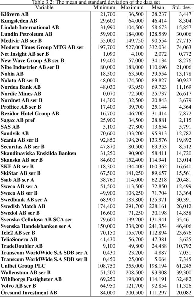
Table 3.2: The mean and standard deviation of the data set

Variable Minimum Maximum Mean Std. dev. Klövern AB 21,700 36,500 28,237 3,447 Kungsleden AB 29,600 64,000 46,414 8,304 Lindab International AB 31,990 104,500 58,673 15,857 Lundin Petroleum AB 59,900 184,000 128,589 30,006 Medivir AB ser B 55,000 149,750 90,554 27,715 Modern Times Group MTG AB ser 197,700 527,000 332,034 74,063 Net Insight AB ser B 1,090 4,100 2,072 0,772 New Wave Group AB ser B 19,400 57,000 34,134 8,276 Nibe Industrier AB ser B 80,000 188,000 110,696 21,006 Nobia AB 18,500 63,500 39,554 13,178 Nolato AB ser B 48,000 174,500 89,827 30,927 Nordea Bank AB 48,030 93,950 69,723 11,169 Nordic Mines AB 0,070 72,500 25,737 26,617 Nordnet AB ser B 14,300 32,500 20,843 3,679 Proffice AB ser B 17,400 39,700 25,144 4,364 Rezidor Hotel Group AB 16,700 46,700 31,414 7,872 Sagax AB pref 25,900 34,500 28,881 2,115 SAS AB 5,100 27,800 13,654 5,791 Sandvik AB 70,600 133,200 95,913 12,782 Scania AB ser B 92,850 198,200 133,576 19,892 Securitas AB ser B 47,870 80,500 63,353 8,512 Skandinaviska Enskilda Banken 31,250 90,900 58,411 14,720 Skanska AB ser B 84,600 152,400 114,941 13,014 SKF AB ser B 118,300 194,400 160,362 16,640 SkiStar AB ser B 67,500 141,250 89,657 15,561 Ssab AB ser A 38,760 114,000 62,218 20,481 Sweco AB ser A 51,500 113,500 72,850 12,499 Sweco AB ser B 49,900 108,250 71,704 13,364 Swedbank AB ser A 68,900 183,800 125,971 30,391 Swedish Match AB 174,400 291,700 228,161 26,012 Swedol AB ser B 16,600 71,250 30,198 14,858 Svenska Cellulosa AB SCA ser 79,600 199,200 131,941 35,461 Svenska Handelsbanken ser A 150,000 338,200 241,354 46,406 Tele2 AB ser B 70,150 155,700 112,894 23,676 TeliaSonera AB 41,430 56,700 47,381 3,625 TradeDoubler AB 9,100 49,800 24,488 10,792 Transcom WorldWide S.A SDB ser A 0,430 23,200 4,887 7,031 Transcom WorldWide S.A SDB ser B 0,450 25,000 5,064 7,345 Unibet Group PLC 108,750 355,000 198,194 61,245 Wallenstam AB ser B 51,500 208,500 93,908 39,300 Wihlborgs Fastigheter AB 69,250 198,000 114,191 32,482 Volvo AB ser B 64,950 121,700 92,854 11,326

(24)

Chapter 4 Procedures in conducting k-means

clustering on a data set

There are several procedures in conducting a k-means clustering. Our procedures entailed of three steps, in its simplest version [12].

Step one: partition of all items into K initial groups

When we use the k-mean clustering method (nonhierarchical method) to analyze our data set, it begins from an initial partition of the items into groups, which forms the nuclei of clusters. Where K points are placed into the space represented by the objects that are being clustered. These points represent initial group centroids. To characterize the data, the method uses K prototypes, the centroid of clusters (classes). These are determined by minimizing the sum of squared errors: N_J = K

∑

j=1i∈C

∑

j (xi− mj)2 (4.1)

where (x1, ...., xn) = D is the set of observations, and mj= ∑i∈Cj

xi

nj is the centroid of class Cj

and njis the number of points in Cj.

For the initial partition, we do not have any information about the clusters. Since, the method initially randomly assigns a class to each observation and then proceeds to the update step, we choose the Random Partition. A random partition of a number n is within the P(n) possible partition of n , where P(n) is the partition function P. Thus, computing the initial mean to be the centroid of the class randomly assigned points.

Step two: Determine the distance of each object to the centroid

Observations that are close together should fall into the same cluster while those that are far apart should be in a different cluster. Theoretically, the observation within a cluster should be relatively homogeneous, but not similar to those contained in other clusters.

Each observation is assigned to the class with the mean that generates the least within-class sum of squares, which is intuitively the nearest mean. Since the sum of squares is the squared

(25)

Euclidean distance. C(t)_j = {xl :k xl− m (t) j k 2_{≤k x} l− m (t) k k ∀k} (4.2)

Where each xl is assigned to precisely one Cj, even in the event that it could be assigned to

more of them.

Step three: Group the objects based on minimum distance

New means are calculated to be the centroids of the observations in the new clusters. m(t+1)_j = 1 | C(t)_j |_x

∑

i∈C (t) j xi (4.3)

This also minimizes the sum of squares objective, since the mathematical mean is the least square estimator.

K-means is a method which, wherever it starts from, converges to a solution. For the ini-tial iteration, a starting point is chosen which consists in associating the center of the k classes with k objects. Thereafter, the distance between the k centers and the objects are computed and the objects are allocated to the centers they are close to. The centers are redefined from the objects allocated to the various classes. The objects are reassigned depending on their distances from the new centers. It continues up to the point that convergence is reached.

4.1 Clustering using the k-means method

Step one: Suppose we measure two variables v1and v2for each of four items M, N, O, and P.

The data are stipulated in the following table

Observation Item v₁ v₂ M 7 3 N -1 1 O 3 -1 P -5 -3

Our aim is to partition these items into K = 2 clusters in order that the items within a cluster are closer to one another than they are to the items in different clusters. We arbitrarily divide the items into two clusters, such as (MN) and (OP), in order to implement the K = 2-means method. Then, we compute the coordinates ( ¯v₁, ¯v₂) of the cluster mean. Therefore, we get the following table.

(26)

coordinates of the centroid Cluster v¯1 v¯2

(MN) 7+(−1)₂ = 3 3+1₂ = 2 (OP) 3+(−5)₂ = −1 −1+(−3)₂ = −2

Step two: We calculate the Euclidean distance of each item from the group centroid and reassign each item the closest group. In the event that an item is moved from the original configuration, the cluster centroid or mean must be updated before continuing. We calculate the squared distances

d2(M; (MN)) = (7 − 3)2+ (3 − 2)2= 17 d2(N; (OP)) = (−1 + 1)2+ (1 + 2)2= 9

coordinates of the centroid Cluster v¯1 v¯2

(M) 7 5 (NOP) −1 −1

We checked each item again for reassignment. Calculating the squared distance provides the following table.

Squared distances to group centroids item

Cluster M N O P (M) 0 68 32 180 (NOP) 100 4 16 20

4.2 Clustering using XLSTAT

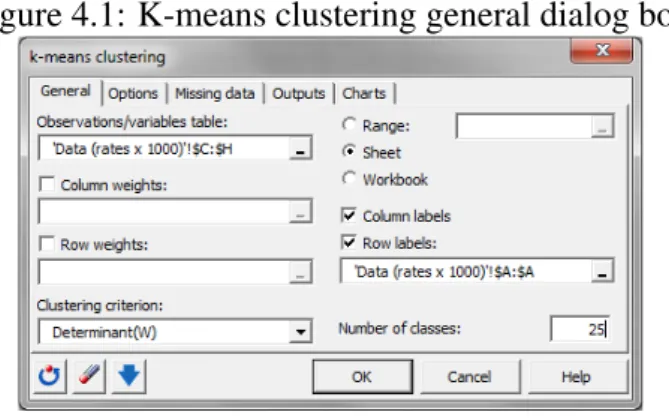
Once the dialog box is open, the data format chosen is the variables or observation because of the format of the input data. Then, we do not activate the column weights and rows weights

(27)

options since we are more particular in the demographic dynamic. There exist several criteria that may be used to come to a solution. XLSTAT offer four criteria to minimized: Trace(W), Determinant(W), Wilks Lamda, and Trace(W)/Median. We select the clustering criterion De-terminant(W) because DeDe-terminant(W) criterion has the propensity to develop clusters of equal shape. Also, the criterions have been found to generate clusters with the approximately equal number of objects. To get the results on a new sheet in the current workbook, we activate the option sheet.

We are clustering stocks, so we activate the option cluster rows because it is the appropri-ate one to use. We do not have any information for the initial partition; therefore, we activappropri-ate the option randomly selected. We increase the number of repetitions to 50, in order to improve the stability and quality of the results. The default stopping condition is good, so we activate the options. In outputs options, we activate all. We activate the evolution of the criterion, which in this case is the determinant(W). Finally, we start the computation by clicking on the OK button. The following window provides the opportunity to double-check the selections before proceeding.

Figure 4.1: K-means clustering general dialog box

Xlstats results

In this section, we will interpret the results generated from our process by using k-means clus-tering method.

4.2.1 Optimization summary

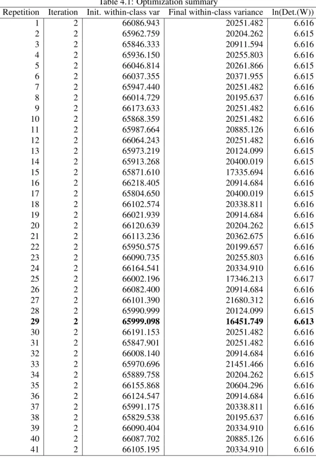
Table 4.1 shows the development of the within-class variance. If several repetitions have been requested, the result of each repetition is displayed.

(28)

Table 4.1: Optimization summary

Repetition Iteration Init. within-class var Final within-class variance ln(Det.(W)) 1 2 66086.943 20251.482 6.616 2 2 65962.759 20204.262 6.615 3 2 65846.333 20911.594 6.616 4 2 65936.150 20255.803 6.616 5 2 66046.814 20261.866 6.615 6 2 66037.355 20371.955 6.615 7 2 65947.440 20251.482 6.616 8 2 66014.729 20195.637 6.616 9 2 66173.633 20251.482 6.616 10 2 65868.359 20251.482 6.616 11 2 65987.664 20885.126 6.616 12 2 66064.243 20251.482 6.616 13 2 65973.219 20124.099 6.615 14 2 65913.268 20400.019 6.615 15 2 65871.610 17335.694 6.616 16 2 66218.405 20914.684 6.616 17 2 65804.650 20400.019 6.615 18 2 66102.574 20338.811 6.616 19 2 66021.939 20914.684 6.616 20 2 66120.639 20204.262 6.615 21 2 66113.236 20362.675 6.616 22 2 65950.575 20199.657 6.616 23 2 66090.735 20255.803 6.616 24 2 66164.541 20334.910 6.616 25 2 66002.196 17346.213 6.617 26 2 66082.400 20914.684 6.616 27 2 66101.390 21680.312 6.616 28 2 65990.999 20124.099 6.615 29 2 65999.098 16451.749 6.613 30 2 66191.153 20251.482 6.616 31 2 65847.901 20251.482 6.616 32 2 66008.140 20914.684 6.616 33 2 65970.696 21451.466 6.616 34 2 65889.758 20204.262 6.615 35 2 66155.868 20604.296 6.616 36 2 66124.547 20914.684 6.616 37 2 65991.175 20338.811 6.616 38 2 65829.538 20195.637 6.616 39 2 66090.404 20334.910 6.616 40 2 66087.702 20885.126 6.616 41 2 66105.195 20334.910 6.616

(29)

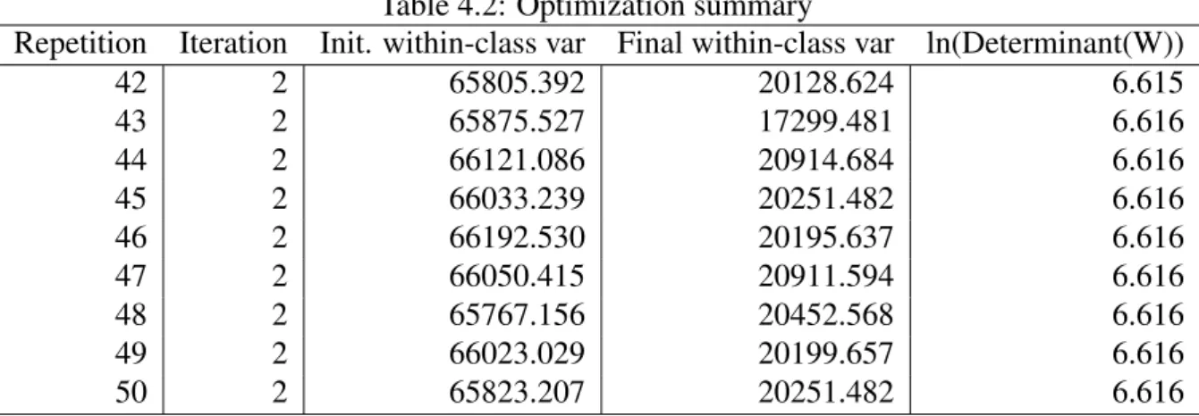
Table 4.2: Optimization summary

Repetition Iteration Init. within-class var Final within-class var ln(Determinant(W)) 42 2 65805.392 20128.624 6.615 43 2 65875.527 17299.481 6.616 44 2 66121.086 20914.684 6.616 45 2 66033.239 20251.482 6.616 46 2 66192.530 20195.637 6.616 47 2 66050.415 20911.594 6.616 48 2 65767.156 20452.568 6.616 49 2 66023.029 20199.657 6.616 50 2 65823.207 20251.482 6.616 The values of Determinant (W) are too big; ln (Determinant (W)) are displayed instead.

4.2.2 Statistics for each iteration

Given the optimum result for the chosen criterion, this option is activated in order to see the development of miscellaneous statistics computed as the iterations for the repetition proceed. A chart showing the development of the chosen criterion as the iterations proceed, if the cor-responding option is activated in the Charts tab. Please note that the results of the optimization summary and the statistics for each iteration are computed in the standardized space if the val-ues are standardized (option in the option’s tab). On the contrary, the following results are displayed in the original space if the result in the original space option is activated.

Table 4.3: Statistics for each iteration

Iteration Within-class variance Trace (W) ln (Determinant (W)) 0 65859.671 58944406 6.637 1 22464.073 20105345 6.620 2 20725.313 18549155 6.619 3 20625.695 18459997 6.619 4 20616.598 18451855 6.619 5 20614.001 18449531 6.619

(30)

Figure 4.2: Statistics for each iteration

4.2.3 Variance decomposition for the optimal classification

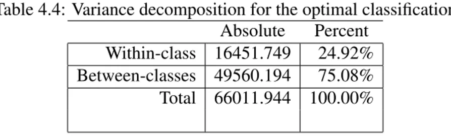
Table 4.4 shows the within-class variance, the between-class variance, and the total variance. The within-class variance is 24,92 percent of the total variance and the between-class variance is 75,08 percent of the total variance. The sum of the within-class variance and the between class variance is the total variance. The within-class variance is the sum of the individual class variance weighted by their respective class probability while the between-class variance is widely used for the original separation of the intensity distribution with regard to the appli-ance of an iterative segmentation method for the reason of diminishing the convergence.

Table 4.4: Variance decomposition for the optimal classification Absolute Percent

Within-class 16451.749 24.92% Between-classes 49560.194 75.08% Total 66011.944 100.00%

A table of the cluster centroids and within-cluster variance also help to explain group differ-ences.

4.2.4 Distance between the class centroid

Table 4.5 shows the Euclidean distances between the class centroids for the various descriptors. It is visible from the table that the Euclidean distances between the class centroid range

(31)

between 482,675 and 189,580. The largest Euclidean distance is between centroid 5 and 1 while the closest is between central objects 3 and 4.

The Euclidean distance is probably the most commonly chosen distance, and it is simply the geometric distance in the multidimensional space.

Table 4.5: Distances between the class centroids

1 2 3 4 5 1 0 1355.916 3203.526 3931.065 4705.046 2 1355.916 0 1909.072 2666.029 3420.408 3 3203.526 1909.072 0 862.382 1523.221 4 3931.065 2666.029 862.382 0 869.263 5 4705.046 3420.408 1523.221 869.263 0

4.2.5 Distance between the central objects

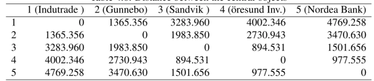
This table indicates the Euclidean distance between the class central objects for the different decriptors. The Euclidean distance between the central objects ranges between 5505,223 to 829.359. The central objects resides in the center of each cluster.

Table 4.6: Distance between the central objects

1 (Indutrade ) 2 (Gunnebo) 3 (Sandvik ) 4 (öresund Inv.) 5 (Nordea Bank) 1 0 1365.356 3283.960 4002.346 4769.258 2 1365.356 0 1983.850 2730.943 3470.630 3 3283.960 1983.850 0 894.531 1501.656 4 4002.346 2730.943 894.531 0 977.555 5 4769.258 3470.630 1501.656 977.555 0

4.2.6 Results by class

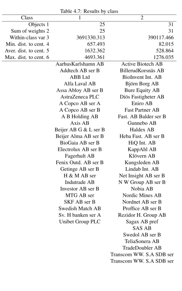
The result by class table shows the descriptive statistics for the classes (number of object, number of weights, within-class variance, the minimum distance to the centroid, the maximum distance to the centroid, mean distance to the centroid). Class one consists of 25 objects of the 85, class two 31, class three 8, class four 11, and class five 10 respectively.

(32)

Table 4.7: Results by class

Class 1 2

Objects 1 25 31

Sum of weights 2 25 31 Within-class var 3 3691330.313 390117.466 Min. dist. to cent. 4 657.493 82.015 Aver. dist. to cent. 5 1632.362 528.864 Max. dist. to cent. 6 4693.361 1276.035

AarhusKarlshamn AB Active Biotech AB Addtech AB ser B BillerudKorsnäs AB

ABB Ltd BioInvent Int. AB Alfa Laval AB Björn Borg AB Assa Abloy AB ser B Bure Equity AB

AstraZeneca PLC Diös Fastigheter AB A Copco AB ser A Eniro AB A Copco AB ser B Fast Partner AB

A B Holding AB Fast. AB Balder ser B Axis AB Gunnebo AB Beijer AB G & L ser B Haldex AB

Beijer Alma AB ser B Heba Fast. AB ser B BioGaia AB ser B HiQ Int. AB Electrolux AB ser B KappAhl AB Fagerhult AB Klövern AB Fenix Outd. AB ser B Kungsleden AB

Getinge AB ser B Lindab Int. AB H & M AB ser Net Insight AB ser B

Indutrade AB N W Group AB ser B Investor AB ser B Nobia AB

MTG AB ser Nordic Mines AB SKF AB ser B Nordnet AB ser B Swedish Match AB Proffice AB ser B Sv. H banken ser A Rezidor H. Group AB

Unibet Group PLC Sagax AB pref SAS AB Swedol AB ser B

TeliaSonera AB TradeDoubler AB Transcom WW. S.A SDB ser Transcom WW. S.A SDB ser

(33)

Table 4.8: Results by class Class 3 4 5 1 8 11 10 2 8 11 10 3 432135.753 398140.386 453224.114 4 223.233 442.370 300.219 5 565.386 576.077 602.866 6 832.123 1027.058 953.448

Atrium Ljungberg AB Bilia AB ser A Boliden AB Ericsson Telefonab Industrial & Fin. Sys. Clas Ohlson AB ser B

Sandvik AB Intrum Justitia AB Medivir AB ser B SkiStar AB ser B JM AB Nolato AB ser B

Tele2 AB ser B Lundin Petroleum AB Nordea Bank AB Wallenstam AB ser B Nibe Indust. AB ser B Securitas AB ser B Wihlborgs Fastigheter AB Scania AB ser B Skand. Enskilda Banken

Volvo AB ser B Skanska AB ser B Ssab AB ser A Swedbank AB ser A Sweco AB ser A Svenska Cell. AB SCA ser Sweco AB ser B

Öresund Investment AB

Result by object Table A.4 shows the assignment class for each object in the initial object order.

We used the table containing the correlation coefficient between each variable to look at the correlation between variables and the others. Our findings reveals that variable in the same cluster are highly positively correlated. When also we look at the correlation of variables in different clusters, they are either highly negatively correlated or lowly positively correlated. This is line with the result we expected. We did this because the cluster are relevant forming our portfolio.

(34)

Chapter 5 Procedures in conducting PCA on a data

set

In this chapter, we will elaborate more on the PCA technique and take you through the steps you needed to perform a Principal Components Analysis on a set of data.

PCA is a useful statistical technique that has found application in fields such as face recogni-tion and image compression, and is a common technique for finding patterns in data of high dimension. First, is to reduce the original variables into a lower number of orthogonal, uncor-related variables or factors. Then, we can look into the variable relationship and look at the correlation between the initial variables, and also between the variables and factors.

Using a data reduction method such as principal component analysis (PCA), reduces the di-mensionality of the data without much loss of information. The first principal components retain most of the variation in the initial variables and to make interpretation simpler, they can be used to describe the relationship between the initial variables and similarities between observations. Principal component analysis is a mathematical technique that reduces dimen-sionality by creating a new set of variables called principal components. The first principal component is the linear combinations of the initial variables and explains as much variation as possible in the initial data. Each subsequent component explains as much of the remaining variation as possible under the condition that it is uncorrelated with the previous components. Though (p) principal components are needed to replicate the whole system variability. Most of this variability can be represented by a small number (k) of the principal components. If it holds, there exists almost as much information on the components as there is in the initial p variables. The k principal components can then replace the original p variables, and the initial data set, comprising of n measurement on p variables, is reduced to a data set comprising of n measurements on k principal components.

An analysis of principal component often indicates a relationship that were not previously suspected. Thereby, allows the clarifications that would not normally result. Analysis of PCA is more of a mean to an end instead of an end in themselves since they often serve as

(35)

in-termediate procedures in much larger inquiries. For instance, a principal component may be inputted to a multiple regression or cluster analysis. They are one factoring of the covariance matrix for the factor analysis model.

Extraction of the initial components

In Principal Component Analysis, the number of principal components is less than or equal to the number of original variables. We extracted 85 variables because our data set entails that number of variables. C_k= p

∑

i=1 u_ikx_i (5.1) The principal components are orthogonal, uncorrelated, and also linear combinations of the initial variables. Ckis both the components and the originally observed variable, and uikin the

contribution of the variable xiin the formation of the component Ck.

Calculating the population principal components

Presume the random variables Y1,Y2, and Y3have the covariance matrix

∑

=   1 −2 0 −2 5 0 0 0 2   It may be shown that the eigenvalue-eigenvector pairs are

λ1= 5.83, e0₁= [0.383, −0.924, 0.00]

λ2= 2.00, e0₂= [0, 0, 1]

λ3= 0.17, e0₃= [0.924, 0.383, 0.00]

So, the principal components become

X₁= e0₁Y = 0.383Y1− 0.924Y2

X₂= e0₂Y = Y3

Y₃= e0₃Y = 0.924Y1− 0.383Y2

The variable Y3 is one of the principle component, since it is uncorrelated with the other two

variables.

Var(X_i) = e0_iΣe0_i= λi i= 1, 2, ..., p (5.2)

Cov(XiXk) = e0iΣe0k= 0 i6= k (5.3)

(36)

Var(X1) = Var(0.383Y1− 0.924Y2)

= (0.383)2Var(Y1) + (−0.924)2Var(Y2)

+2(0.383)(−0.924)Cov(Y1,Y2)

= .147(1) + 0.854(5) − 0.708(−2) = 5.83 = λ1

Cov(X1, X2) = Cov(0.383Y1− 0.924Y2,Y3)

= 0.383Cov(Y₁,Y₃) − 0.924Cov(Y₂,Y₃) = 0.383(0) − 0.924(0) = 0

It is also clearly obvious that

σ11+ σ22+ σ33= 1 + 5 + 2 = λ1+ λ2+ λ3= 5.83 + 2.00 + 0.17

showing

Total variance= σ11+ σ22+ ... + σpp

= λ1+ λ2+ ... + λp

for the example. The fraction of total variance accounted for by the first principal component is λ1/(λ1+ λ2+ λ3) = 5.83/8 = .73. Additional, the first two components account for a fraction

(5.83 + 2)/8 = 0.98 of the population variance. In this situation, the components X1 and X2

could restore the initial three variables with little loss of information. using ρXi,Yk= e_ik√λi √ σ_kk i, k = 1, 2, ..., p we obtain ρX1,Y1 = e₁₁√λ1 √ σ11 = .383 √ 5.83 √ 1 = 0.925 ρX1,Y2 = e₂₁√λ1 √ σ22 = −0.924 √ 5.83 √ 5 = −0.998

See here that the variable Y2with coefficient −0.924 obtains the most weight in the component

X₁. In absolute value, it has the largest correlation with X1. The correlation of Y1and X1, 0.925

is roughly as large as that for Y2showing that the variables are almost equally important to the

first principal component. The comparative sizes of the coefficients of Y1 and Y2suggest, on

the other hand, that Y2add more to the determination of X1than Y1does. But, in this situation,

both coefficients are fairly large and of opposite signs, we should argue that both variables help in the reading of X1. Lastly,

ρX2,Y1= ρX2,Y2 = 0 and ρX2,Y3 = √ λ2 √ σ33 = √ 2 √ 2= 1

The third component is irrelevant, and because of this the remaining correlations can be neg-lected.

(37)

5.1 PCA using software application

First, we need to open the dialog box of the function PCA through the menu analyzing data. Once the dialog box is open, observation or variable is the data format chosen as a result of the format of the input data. The Pearson’s correlation matrix is the PCA type we activate, which tallies, to the classical correlation coefficient. To get the results on a new sheet in the current workbook, we activate the option sheet. In the input tab, we activate the option to display significant correlations in bold characters (Test significance). The filtering option is unchecked, in order to display the labels on all charts, and moreover to display all the observa-tions (observation charts and bi-plot) in the chart. Since filtering the observaobserva-tions might make the results unreadable. In the final stage, we are required to confirm the number of columns and rows. The computations begin at the moment we click OK.

5.1.1 Interpretation of the PCA results

In this section, we interpret the results we generated after running our data in the PCA system. The eigenvector and eigenvalue

In Table 5.1 the eigenvalues and percentage of the total variance for each and every compon-ent describe the extracted principal componcompon-ents. The number of dimensions the data set has is equal to the amount of eigenvectors or eigenvalues that exist. The eigenvectors and eigen-values exist in pairs and it signifies that every eigenvector has a corresponding eigenvalue. An eigenvector is a direction while an eigenvalue is a number telling you how much variance exists in the data in that direction. The first principal component is the eigenvector with the largest eigenvalue. In table 5.1, the first factor has the optimal amount of 0.39 percent of the total variance in the observed variables and correlated with a number of the original variables. For that being the case, the first factor is the principal component, followed by the second, third, fourth and fifth respectively.

Table 5.1: Eigenvalues

F1 F2 F3 F4 F5 F6 F7 F8 Eigenvalue 32,468 27,117 8,610 3,950 3,370 1,460 1,384 0,992 Variability (%) 38,197 31,902 10,130 4,647 3,965 1,718 1,629 1,167 Cumulative % 38,197 70,099 80,229 84,876 88,841 90,559 92,188 93,355 The factor loading of the Principal Component Analysis, which reflects on the amount that the variable contributes to that respective principal component. Factor loading represents how much a describes a variable in a factor analysis. The factor loading consist of three categories; those considered strong are greater than 0.75, those considered moderate are between 0.75 and 0.50, and those considered weak are between 0.49 and 0.30. Those that are less 0.30 are negligible. In our report analysis, we selected only strong factors for the principal component

(38)

interpretation. Three factors extracted from the principal components indicate a total variabil-ity of 71.8 % of our data set.

The number of principal components

To determine the amount of components to retain, there exist things to take into consideration. This includes the relative size of the eigenvalue, the number of total sample variance, and the subject-matter interpretations of the components. Important to note is that, a component with an eigenvalue close to zero and deemed insignificant, may show an unexpected linear depend-ency in the data.

Scree Plot

The scree plot is a very significant aid in determining the suitable number of components or factors to retain. Figure 5.1.1shows a scree plot which consists of 85 principal factors, and with eigenvalue ranked from largest to the smallest. We look for a bend or elbow in the scree plot, in order to know the actual number of components to retain. The number of components is deemed to be the point at which the outstanding eigenvalues are all about the same size and being relatively small. In the Scree Plot that we generated from our data set, an elbow prevails precisely at factor 5. That is to say that the eigenvalues for factor 6 and below are all approximately the same size and being relatively small. In that regards, there exist three sample principal components which in actual fact summarize the total sample variance.

Figure 5.1: The Scree plot

Interpretation of the factors

Interpreting a factor signifies what phenomenon is measured by this factor or identifying the significance of this factor. Therefore, factors that we retain are those that we can interpret. In order to retain a factor, there must be at least some original variables that are strongly correl-ated with this factor. In our analysis, we retain the first three factors for interpretation.

(39)

There exist three dominant principal components (F1;F2;F3), which explain 84,44 percent of the total variance. Therefore, has an interesting subject-matter interpretation since they are considered as the strongest factors. For the interpretation of a factor or component, we will look for the most strongly correlated variables with the factor, and specify what these variable possess in common. The correlation between the factors and the observed variables are the factor loading.

Factor loadings signify how much a factor describes a variable in factor analysis. For in-stance, a survey is conducted each survey question, check the highest (positive or negative) loading to find out which factor affects the question most. Loading can vary from -1 to 1. Loading close to -1 or 1 highlights that the factor strongly affects the variable. Loading close to zero highlights that the factor has a limited effect on the variable.

(40)

Table 5.2: Factor loading F1 F2 F3 F4 F5 AarhusKarlshamn AB 0,661 -0,648 -0,282 -0,164 -0,017 Active Biotech AB 0,336 0,266 0,717 -0,172 -0,176 Addtech AB ser B 0,542 -0,368 0,047 0,322 0,225 ABB Ltd 0,522 0,148 0,147 -0,329 0,597 Alfa Laval AB 0,728 -0,619 0,146 0,022 0,156 Assa Abloy AB ser B 0,714 -0,666 -0,120 -0,116 -0,040 AstraZeneca PLC 0,564 -0,026 -0,115 -0,313 -0,537 Atlas Copco AB ser A 0,816 -0,240 -0,050 0,371 -0,284 Atlas Copco AB ser B 0,827 -0,193 -0,071 0,353 -0,309 Atrium Ljungberg AB ser B 0,464 0,360 -0,269 0,325 -0,570 Avanza Bank Holding AB 0,560 -0,357 0,644 -0,220 -0,111 Axis AB 0,757 -0,500 -0,178 0,061 0,270 Beijer AB G & L ser B 0,265 0,479 0,545 0,366 -0,102 Beijer Alma AB ser B 0,746 -0,574 0,212 -0,054 -0,051 Bilia AB ser A 0,926 -0,188 0,138 0,016 0,017 BillerudKorsnäs AB 0,869 0,310 -0,228 0,165 0,010 BioGaia AB ser B 0,430 -0,870 -0,026 0,098 -0,007 BioInvent International AB -0,369 0,580 0,636 -0,163 -0,077 Björn Borg AB 0,260 0,869 0,082 0,012 0,164 Boliden AB 0,812 0,166 0,227 0,324 -0,102 Bure EquBity A 0,092 -0,799 -0,001 -0,297 0,227 Clas Ohlson AB ser B 0,551 0,601 0,046 -0,338 -0,030 Diös Fastigheter AB 0,899 -0,317 0,050 -0,037 0,001 Electrolux AB ser B 0,706 -0,172 0,321 -0,081 -0,164 Ericsson Telefonab L M ser 0,609 0,608 -0,164 0,076 -0,142 Eniro AB 0,535 0,682 -0,386 -0,096 0,025 Fagerhult AB 0,647 -0,531 -0,194 0,010 0,142 Fast Partner AB 0,732 -0,634 -0,152 -0,076 -0,011 Fastighets AB Balder ser B 0,402 0,678 -0,319 -0,336 -0,023 Fenix Outdoor AB ser B 0,554 -0,770 0,146 -0,204 -0,054 Getinge AB ser B 0,674 -0,546 -0,107 0,110 0,215 Gunnebo AB 0,573 0,755 -0,130 0,102 0,182 Haldex AB 0,507 0,815 -0,049 0,004 0,056 Heba Fastighets AB ser B 0,486 0,708 -0,335 0,156 0,189 Hennes & Mauritz AB H & M ser 0,690 -0,564 0,191 -0,175 -0,059 HiQ International AB 0,920 -0,043 0,079 0,107 0,139 Industrial & Financial Systems 0,313 -0,868 0,218 -0,107 -0,125 Indutrade AB 0,766 -0,613 0,095 -0,049 0,048 Intrum Justitia AB 0,665 -0,506 -0,283 -0,269 0,147 Investor AB ser B 0,849 -0,259 -0,325 -0,224 0,041 JM AB 0,966 0,119 -0,038 0,044 -0,020 KappAhl AB 0,315 0,792 0,076 -0,442 -0,063

(41)

F1 F2 F3 F4 F5 Klövern AB 0,889 -0,089 0,285 0,083 -0,050 Kungsleden AB 0,525 0,778 -0,097 0,203 -0,114 Lindab International AB 0,370 0,868 -0,124 -0,059 0,249 Lundin Petroleum AB 0,391 -0,697 -0,225 0,405 0,177 Medivir AB ser B 0,386 -0,240 0,783 -0,170 -0,076 Modern Times Group MTG AB ser 0,551 0,457 0,565 0,038 -0,170 Net Insight AB ser B -0,097 0,943 0,067 -0,125 -0,088 New Wave Group AB ser B 0,730 0,615 -0,017 0,130 0,157 Nibe Industrier AB ser B 0,837 -0,347 -0,113 0,050 -0,159 Nobia AB 0,511 0,548 -0,217 0,212 -0,499 Nolato AB ser B 0,746 -0,507 -0,082 -0,334 -0,095 Nordea Bank AB 0,621 0,625 -0,309 -0,163 0,196 Nordic Mines AB -0,076 0,257 0,708 0,420 0,088 Nordnet AB ser B 0,734 -0,015 0,346 -0,300 -0,198 Proffice AB ser B 0,663 -0,197 0,616 0,129 -0,103 Rezidor Hotel Group AB 0,818 0,496 -0,028 0,009 0,003 Sagax AB pref 0,803 -0,353 -0,326 0,027 0,056 SAS AB 0,261 0,824 -0,407 0,148 0,087 Sandvik AB 0,759 0,354 0,262 0,248 0,312 Scania AB ser B 0,579 0,462 -0,215 0,322 -0,460 Securitas AB ser B 0,407 0,812 -0,131 -0,118 -0,095 Skandinaviska Enskilda Banken 0,446 0,740 -0,435 0,096 0,174 Skanska AB ser B 0,921 0,237 0,148 -0,046 -0,052 SKF AB ser B 0,805 -0,395 0,342 0,172 0,048 SkiStar AB ser B 0,208 0,556 0,626 -0,295 -0,136 Ssab AB ser A 0,182 0,923 -0,030 -0,025 0,256 Sweco AB ser A 0,540 0,401 -0,314 0,254 -0,527 Sweco AB ser B 0,762 -0,513 -0,176 -0,140 0,178 Swedbank AB ser A 0,777 0,365 -0,437 0,150 0,155 Swedish Match AB 0,326 -0,784 0,182 0,370 0,102 Swedol AB ser B 0,286 0,575 0,657 0,053 0,217 Svenska Cellulosa AB SCA ser 0,786 -0,438 -0,301 -0,195 0,020 Svenska Handelsbanken ser A 0,795 -0,519 -0,108 -0,186 -0,002 Tele2 AB ser B 0,245 0,253 0,651 0,451 0,328 TeliaSonera AB 0,666 0,475 0,235 -0,037 0,065 TradeDoubler AB 0,262 0,902 -0,265 0,122 0,064 Transcom WorldWide S.A SDB ser 0,085 0,972 -0,036 -0,076 -0,089 Transcom WorldWide S.A SDB ser 0,098 0,970 -0,039 -0,079 -0,102 Unibet Group PLC 0,643 -0,210 -0,464 -0,408 0,055 Wallenstam AB ser B 0,459 0,607 0,443 -0,221 -0,065 Wihlborgs Fastigheter AB 0,381 0,405 0,609 -0,278 -0,195 Volvo AB ser B 0,841 0,252 0,131 0,240 0,295 Öresund Investment AB 0,789 0,451 -0,129 -0,238 -0,058

(42)

The map is identified as the correlation circle. It highlights the projection of the original variables in the factor space. When two variables are distances from the center, then, in the event that they are: orthogonal, they are not correlated; when they are close to each other, they are considerably positively correlated; if they are on the opposite side of the center, then they are considerably negatively correlated.

When some information is carried on the axes, it signifies that the variables are nearer to the center and that any interpretation might be risky. For instance, we might be persuaded to interpret two variables when in actual fact doing an interpretation is hard or not possible to do in such a way. This can be verified by looking at the correlation matrix. To collaborate that a variable is rightly linked with the axes, we have to take a look in the squared cosines table. The closer the squared cosine of a particular variable is to zero, the more attentive you have to be when interpreting the results relating to trend on the corresponding axis.

Figure 5.2: Correlation between circles and factors

To determine the variables which contribute the most to the components, we used the con-tribution matrix. The observations contribute more to the component when the values of the contribution are larger. In Appendix B.3, it is visible that, the contributions of the observations to the factors are not so strong.

Using k-means and PCA in construction of a stock portfolio

MASTER (1 YEAR) THESIS IN MATHEMATICS / APPLIED MATHEMATICS