An outline for a validation database for SAMGODS

(1)

www.vti.se/publikationer

Rune Karlsson Inge Vierth Magnus Johansson

An outline for a validation database

for SAMGODS

VTI notat 30A–2012 Utgivningsår 2012

(2)

(3)

Preface

This study constitutes a first step (pilot study) towards the development of a validation database for output data from goods transport models such as the SAMGODS model. Here, the basic design for the prospective database is described.

In a later step, a prototype of the validation database will be developed before the final database is created.

The Swedish Transport Administration (STA) has commissioned the Centre for Transport Studies (CTS) to develop a validation database. Both VTI and Trafikanalys are parts of CTS. Contact persons at the STA are Carsten Sachse and Petter Hill.

Project leader is Inge Vierth. The first two authors are employed at VTI, while the third author, Magnus Johansson, is employed at Trafikanalys.

Linköping, July 2012

(4)

Kvalitetsgranskning

Intern peer review har genomförts 21 juni 2012 av Jenny Karlsson. Rune Karlsson har genomfört justeringar av slutligt rapportmanus. Projektledarens närmaste chef Gunnar Lindberg har därefter granskat och godkänt publikationen för publicering 30 juli 2012. Större delen av den engelska texten har språkgranskats av Pamela Vang.

Quality review

An internal peer review was performed on 21 June 2012 by Jenny Karlsson. Rune Karlsson has made alterations to the final manuscript of the report. The research director of the project manager Gunnar Lindberg examined and approved the report for

(5)

Summary

A new Swedish national goods transportation model, SAMGODS, has been developed through collaboration among Swedish transport authorities.

As the model recently has begun to be applied to real world problems, the need for a validation database has increased. The purpose of such a database is to facilitate validations of the model.

The current paper presents a pilot study to create a validation database for SAMGODS. The study focuses on two areas: available data sources that may provide validation data, and how to carry out the validation in practice. The latter is of particular importance since a large number of practical problems arise when matching SAMGODS output data with the validation data. Worth mentioning among the problems that arise are: the inhomogeneous structure of the data tables, the often differing aggregation levels

between model output data and validation data, differing time periods, differing systems for commodity groups and elasticities not being immediately available from the

SAMGODS data. Other complicating issues are handling of confidential data and the large quantities of data.

In this report, a relatively detailed proposal for the design of a validation database is put forward. However, the proposed design is not limited to SAMGODS output data, but it is hoped to be sufficiently flexible to comprise also other goods transportation data from future regional or local models. One of the main ideas in designing the database has been to develop a uniform and flexible data table format in which all relevant data can be stored. This format greatly facilitates the matching between SAMGODS output data and the validation data. Other problems and associated possible solutions are thoroughly discussed.

(8)

(9)

Utformning av en valideringsdatabas för SAMGODS

av Rune Karlsson, Inge Vierth och Magnus Johansson* VTI

581 95 Linköping

Sammanfattning

En ny svensk nationell godstransportmodell, SAMGODS, har utvecklats i ett samarbete mellan svenska transportmyndigheter. Under senare tid, då detta system har börjat komma till användning i utredningar, har behovet av en valideringsdatabas vuxit sig allt starkare. Syftet med en sådan databas är att samla alla typer av data som kan användas för validering av modellen samt att underlätta själva valideringsprocessen, det vill säga jämförandet mellan utdata från SAMGODS och (oberoende) externa data.

Detta notat presenterar en förstudie för, och ett första steg mot, skapandet av en valideringsdatabas för SAMGODS-systemet. Förstudien fokuserar på två delar; dels vilka datakällor som kan finnas tillgängliga för valideringen, dels hur man kan utforma verktyg som kan användas för att smidigt och enkelt genomföra den. Den senare delen är väsentlig eftersom där föreligger en lång rad praktiska svårigheter vid matchningen mellan SAMGODS-utdata och valideringsdata, vilka riskerar göra valideringsarbetet både tidskrävande och omständligt. Bland sådana svårigheter kan nämnas: den in-homogena strukturen på datatabellerna, de ofta olika avgränsningarna och aggregerings-nivåerna mellan modelldata och valideringsdata, de ibland även skilda tidsperioderna och skilda systemen för varugruppsindelningar samt att elasticiteter inte omedelbart erhålls från SAMGODS-utdata och som dessutom inte alltid är överförbara mellan olika länder/regioner. Ytterligare problem utgör hanteringen av konfidentiella data samt de stora datamängderna.

I notatet läggs ett relativt detaljerat förslag fram över hur en valideringsdatabas för SAMGODS kan utformas. Designen av databasen är dock inte begränsad till

SAMGODS utan är förhoppningsvis tillräckligt flexibel för att kunna tillämpas även på andra godsmodeller såsom regionala och lokala. En grundläggande idé är att använda ett enhetligt men flexibelt tabellformat för alla relevanta data. Detta format underlättar matchningen mellan SAMGODS-utdata och valideringsdata. Övriga ovan nämnda problem diskuteras utförligt och förslag på hur de kan hanteras framläggs. Det diskuteras även olika möjligheter att ta till vara resultaten från jämförelserna mellan modellresultat och avstämningsdata.

(10)

(11)

1 Introduction

During the development of the Swedish goods transportation model for long distance national and international freight transports (SAMGODS), an increasing need for tools for assessing the system and for systematically evaluating its output has been

recognized. The Swedish Transport Administration (Trafikverket) therefore

commissioned CTS to develop a validation database1, a tool for facilitating comparisons between model outputs and independent statistical data, traffic counts, etc. The

development of such a validation database is especially interesting for freight transports as there is a bench of different official statistics above the traffic counts of vehicles. A validation database can be valuable from a number of perspectives. Firstly,

comparisons between model output data and validation data can conveniently be made in a systematic and comprehensive way rather than checking individual validation cases separately. Secondly, it can give direct indications about the quality of the model output data; this should facilitate the work of identifying programming bugs or other

deficiencies in the model. Thirdly, it can conveniently provide a rich set of calibration data. Fourthly, it can help to determine the resolution or aggregation level at which results can be expected to be reasonably reliable and acceptable. Fifthly, such a database may give hints for suitable future developments of the system. Finally, the database might not only be used for comparing model output data with statistical data, but also for comparing the output from different model versions (or scenarios). For example, if some (sub-) model of the SAMGODS model system has been modified or replaced, then the validation database could be used for easy surveillance and evaluation of the differences between the two models, similar to the comparison between the model output data and the validation data. It is even possible to imagine comparing output from entirely different goods models. For instance, it might be interesting to compare the outcome from SAMGODS and the European model, TRANSTOOLS, or to compare SAMGODS with a local model such as GORM for the Öresund region. A further

possibility would be to include a function for comparing statistical data from different years.

There are a number of challenges to make the data sources comparable. Firstly, both model output and statistical data are stored in many different tables with a number of different formats. Secondly, the aggregation levels of the data have to agree. This is true not only in the spatial sense but also with regard to commodity groups and vehicle classes. Thirdly, the time periods have to agree. A further problem is that there exist different classification systems for commodity groups. Finally, the important problem of protecting sensitive or confidential data has to be dealt with.

Once the matching between the model output data and the validation data has been carried out, the problem of evaluating the rather large set of data that is generated during the comparisons remains. Various measures could be defined that concisely describe the deviation between the model results and the validation data and that give a concise evaluation of the quality of a model. The construction of appropriate such measures is an important part of the validation database.

In the current study, we discuss these problems in more detail and provide an outline for a possible design for a validation database. Although the SAMGODS model has been

1

One may hesitate about what is the most appropriate denomination: a validation database or a validation tool. A requirement has been that it should be a tool for facilitating validations for model output. Another requirement has been that it should also comprisevalidation data.

(12)

very much in focus during the work, we believe that the suggested design of the validation database is sufficiently general to be able to host output data from other goods models as well.

(13)

2 Purpose and limitations

More specifically, the purpose of this study is to:

• prepare the way for the development of a database for validation of SAMGODS output data (that comprises long distance national and international freight transports) as well as Swedish goods models in general (in particular regional models, but also international models such as TRANSTOOLS)

• identify and illustrate difficulties and obstacles encountered when designing such a database and to suggest solutions to these challenges

• give an idea of what types of data that can be stored in the database • suggest what kind of functionalities the database can perform.

One demand is that the work should be guided by, but not limited or restricted to, the current SAMGODS model. The structure in the validation database should be

sufficiently general to be able to host data from future regional or local goods models. In a broader sense, a “validation database” might also include model input data. However, questions concerning the quality of input data do not depend on the model itself and are therefore not discussed in this report.

The validation database can provide data for calibration of the models. This topic is beyond the scope of the current study.

(14)

3 The SAMGODS model and its output data

3.1 Brief description of the SAMGODS system

The Swedish national freight model system, SAMGODS, is used for simulating the goods transport in the short run (representation of the base year, transport policy simulations) as well as the long run (forecasting for scenarios, providing input for the assessment of infrastructure projects). Before 2005, the SAMGODS model was developed as a traditional 4-step model and was implemented in a STAN program environment2. The model had no logistic elements such as the determination of shipment size or the use of consolidation and distribution centers. Since 2005 a new model3 that includes logistics decisions at the level of individual firms has been under development. The new model has begun to be applied to real-world problems during the last couple of years.

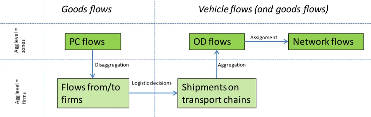
The new SAMGODS model can be described as an aggregate-disaggregate-aggregate (ADA) model system (see Fig 3.1). The first step of the model system consists of determining the freight demand between production and consumption zones, including intermediate whole-sales zones. This is done for 34 commodity groups. These PWC4 matrices are then disaggregated to “firm level” by dividing the demand into three size class levels of firms (small, medium and large)5. In a second step, optimal shipment sizes and optimal transport chains, including the mode and vehicle type of the carrier, are computed. In a third step, these are gathered and collected into OD flows of vehicles or goods. Finally, the vehicle flows are assigned to the network.

Figure 3.1 ADA structure of the SAMGODS system. The top level displays aggregate models while disaggregate models are at the bottom level. The models in the left hand boxes describe goods flow, while in the right boxes both vehicle and goods flows are computed.

2

See (SIKA, 2001)

3

See (de Jong, G.; Ben-Akiva, M.; Baak, J., 2008), (Vierth, I; Lord, N; McDaniel, J, 2009), SAMGODS/CUBE manual.

4

Production – Whole-sale – Consumption.

5

There are 10 different subcells of firms (3 x 3 + one subcell for singular flows) and 34 commodity groups and, hence, altogether 340 base matrices.

PC flows OD flows Network flows

Flows from/to firms Shipments on transport chains Disaggregation Aggregation Logistic decisions Assignment

Goods flows Vehicle flows (and goods flows)

A g g le v e l = zo n e s A g g le v e l = fi rm s

(15)

The transformation of PWC flows between firm classes into OD flows of vehicles is performed by the so called logistics model. It consists of four sub-programs:

• BUILDCHAIN: a program to generate the available transport chains (including the optimal transfer locations between OD legs)

• CHAINCHOICE: a program for the choice of the optimal shipment size and optimal transport chain (including the number of OD legs)

• EXTRACT: programs to extract cost data for specific relations and to extract OD matrices.

• MERGE: is used to merge the commodity specific output.

The logistics model has been implemented in an independent program by the Dutch consultancy firm, Significance. This program was later imbedded into a CUBE interface.

3.2 Output data from SAMGODS

In this section, an overview of the output data generated by the SAMGODS model is presented. Output is generated in two different file formats: text files generated directly by the logistics module and .mdb files generated by the SAMGODS CUBE interface. The CUBE interface reads the text files and transforms them into Access tables. 3.2.1 Text files generated by the logistics module

When running the logistics module for a specific scenario, four main procedures generate output files that may be of interest for validation purposes:

Build chain:

Essentially, this routine selects the best possible (cheapest) transport chain, per commodity group and chain type, for each origin – destination pair.

For each commodity group, a file6 is generated, describing, for each pair of zones, all the computed chains between the zones. For each such chain, the chain type is stated as well as the FromNode and ToNode for each leg in the chain.

Chain choice:

Essentially, this routine computes optimal transport solutions (flows) on the selected chains.

A number of files are generated for each commodity group and each chain. These contain a number of quantities for the chain: tonnes, number of shipments, various types of costs.

(16)

Extract:

This routine computes three OD-matrices7, for each vehicle type: one for the flows of tonnes, one for the number of loaded vehicles and one for the number of empty vehicles.

3.2.2 Results stored in an Access database

A great feature of the SAMGODS CUBE interface is that all, or at least most of the SAMGODS output data, for a specific scenario, is collected in one MS Access file8. The data is stored in a large number of tables in this .mdb file. Each table has its own

structure and format. Usually, different tables are used for storing data with different aggregation levels.

Network data:

Most of the computed link quantities are stored in one9 table: Loaded_Net_X_Link, where X denotes the commodity group. For each link in the network and each vehicle type, the table contains three computed quantities: tonnes, number of loaded vehicles and number of empty vehicles. It also contains aggregations to main modes and totals. Aggregated tables:

A rather large set of output quantities at different aggregation levels are stored in the tables: Report1_xxx,… , Report 11_xxx and the tables CHAIN_OD_COV_xxx and VHCL_OD_COV_xxx. These tables are very useful for comparisons with validation data.

3.2.3 Example of an output table

In Table 3.1 an example of (part of) an output table containing aggregated data is

shown. The column headers contain variable names, while rows contain vehicle classes.

7

The OD-matrices are stored in files named: OD_yyyxxx_z.314, where yyy is either Tonnes, Emp or Vhcl, xxx is the vehicle type number and z is the commodity number.

8

The name of this file has the syntax: Outputx_sce.mdb, where x is a digit, signifying which product groups has been run (0=all products), and sce denotes the name of the scenario.

9

(17)

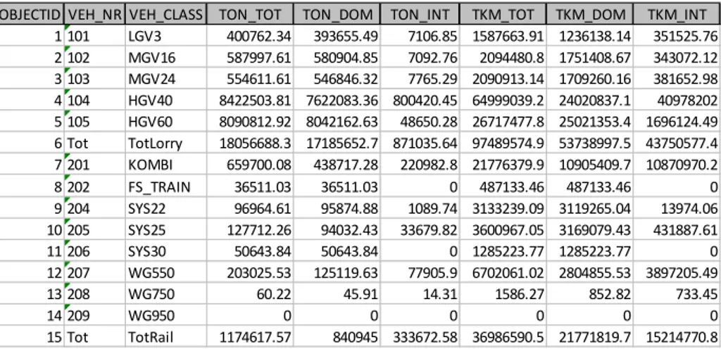
Table 3.1 The output table Report4_xxx from SAMGODS. Tons and tonkm aggregated to total, domestic (=Swedish) and international geographic level for various vehicle types. Only road and rail vehicle modes are shown in the table.

The table efficiently stores data that expresses one particular aspect: total quantities per vehicle class aggregated to national/international level. Each of the other output tables expresses some other aspect. The data is spread over a (large) number of such tables. This fragmentary picture complicates any comparisons between model output data and validation data, especially when the aggregation levels disagree.

3.2.4 Results from scenario comparisons

In the SAMGODS interface there is an application called “Compare scenario”, which can perform a comparison between the current scenario and any other scenario that has been run. The Compare scenario produces flow differences on links for all vehicle types. These differences are stored in a special table

COMPARE_LOADx_Sce1_Sc2_Link, where x is the commodity group, and Sce1 and Sce2 are the names of the two scenarios to be compared.

OBJECTID VEH_NR VEH_CLASS TON_TOT TON_DOM TON_INT TKM_TOT TKM_DOM TKM_INT 1 101 LGV3 400762.34 393655.49 7106.85 1587663.91 1236138.14 351525.76 2 102 MGV16 587997.61 580904.85 7092.76 2094480.8 1751408.67 343072.12 3 103 MGV24 554611.61 546846.32 7765.29 2090913.14 1709260.16 381652.98 4 104 HGV40 8422503.81 7622083.36 800420.45 64999039.2 24020837.1 40978202 5 105 HGV60 8090812.92 8042162.63 48650.28 26717477.8 25021353.4 1696124.49 6 Tot TotLorry 18056688.3 17185652.7 871035.64 97489574.9 53738997.5 43750577.4 7 201 KOMBI 659700.08 438717.28 220982.8 21776379.9 10905409.7 10870970.2 8 202 FS_TRAIN 36511.03 36511.03 0 487133.46 487133.46 0 9 204 SYS22 96964.61 95874.88 1089.74 3133239.09 3119265.04 13974.06 10 205 SYS25 127712.26 94032.43 33679.82 3600967.05 3169079.43 431887.61 11 206 SYS30 50643.84 50643.84 0 1285223.77 1285223.77 0 12 207 WG550 203025.53 125119.63 77905.9 6702061.02 2804855.53 3897205.49 13 208 WG750 60.22 45.91 14.31 1586.27 852.82 733.45 14 209 WG950 0 0 0 0 0 0 15 Tot TotRail 1174617.57 840945 333672.58 36986590.5 21771819.7 15214770.8

(18)

4 Validation data

4.1 What types of possible validation data exist?

What types of data exist that could be used for the validation of results from national or regional goods transportation models? This question is meant in a broader sense; what data might exist and not only what data does exist. Important to us is not only which variables are relevant but also the mathematical structure of the data.

Validation data can be characterized on the basis of a number of different aspects or dimensions. In order to get an overview over the possibilities we try to describe the most important aspects of goods transportation data. Almost any combination of the aspects below could be possible.

• The unit of the data

E.g.: Loaded tons, tonkm, vehicle-km, number of vehicles, load factor, energy consumption [kWh], emission of particles measured in [g]. • The aggregation level

Spatial aggregation level: National level data, regional level data, municipal level data, zonal data, links, node data (e.g. in ports or terminals), transport chains, etc.

Commodity aggregation level

Aggregation level for modes or carriers: e.g: Rail, Wagon load (WG550 tons), individual wagons in a train, etc. Loading units (containers, pallets etc.) can also be included here.

• Time period

The above list of aspects can be made longer; for instance, Swedish registered or foreign vehicles, Loaded or empty vehicles, etc.

One can also distinguish between given validation data values and given feasible intervals. A feasible interval may specify the upper and lower limits within which a value is acceptable.

Besides individual values, validation data might also include probabilities and distributions of variables, e.g. route lengths for a specific vehicle type.

4.2 Elasticities

Elasticities (i.e. “relative derivatives”) constitute a rather special group of validation data. An elasticity represents the impact of a change in an independent (or stimulus) variable on a dependent (or response) variable, both measured in percentage changes. There are a large number of possible elasticities. The stimulus variable may typically be some sort of cost, but may also be some property of the vehicles (e.g. the capacity of some train type). The response variable can be virtually anything, from aggregated quantities such as total tonkm for heavy goods vehicles in Sweden, to disaggregated link flows in an entire network. Examples of frequently used elasticities are: own price elasticities, cross price elasticities and time elasticities.

(19)

Often, validation data are not known as exact elasticities but are instead given in the form of upper and lower limits for what is a reasonable value.

Elasticities10 usually come from theoretical models (econometric models and transport models), which are based on empirical data, but in some cases, elasticities can be calculated from direct observations of the impact of a change (e.g. introduction of a toll), from before and after studies. The data used for model estimation can be time series data, cross section data or panel data. If a time-series model contains lagged parameters, the model can distinguish between short and long term effects. Whether the effects from a cross section are short or long term depends on a judgement on the nature of the behavioural mechanisms included (e. g. location decisions are regarded as long run).

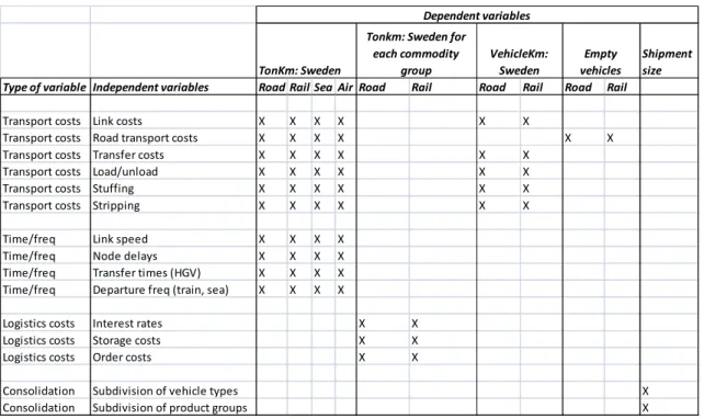
There is an abundance of possible combinations between independent and dependent variables. In (Trafikanalys, 2011) a list of the most relevant elasticities is proposed. In Table 4.1 an overview of these is given.

Table 4.1 Examples of elasticities that should be validated, according to Trafikanalys.

It is important to note that elasticities taken from the literature may not be applicable to other cases, since circumstances can vary, for example, among countries, or even

regions. Moreover, it should perhaps not be expected that a national transport model can replicate an externally estimated elasticity since the model may suffer from limitations in adaptability.

10

Reference for road elasticities: (de Jong, Schroten, van Essen, Otten, & Bucci, 2010) Reference for rail elasticities: (Vierth, Mellin, Hylén, de Jong, & Bucci, 2010)

TonKm: Sweden

Shipment size Type of variable Independent variables Road Rail Sea Air Road Rail Road Rail Road Rail

Transport costs Link costs X X X X X X

Transport costs Road transport costs X X X X X X

Transport costs Transfer costs X X X X X X

Transport costs Load/unload X X X X X X

Transport costs Stuffing X X X X X X

Transport costs Stripping X X X X X X

Time/freq Link speed X X X X

Time/freq Node delays X X X X

Time/freq Transfer times (HGV) X X X X

Time/freq Departure freq (train, sea) X X X X

Logistics costs Interest rates X X

Logistics costs Storage costs X X

Logistics costs Order costs X X

Consolidation Subdivision of vehicle types X

Consolidation Subdivision of product groups X

Empty vehicles VehicleKm:

Sweden Tonkm: Sweden for

each commodity group

(20)

4.3 Confidential data

A special category of validation data is data that needs to be protected. Any data that may reveal the transportation strategy for an individual company can potentially be regarded as confidential.

For freight companies, examples of these data might be: route information, the load or load factors on individual vehicles, the cost for transports or the value of the goods. For terminals and ports, data such as total number of tons transferred annually may be confidential, in particular when separated into individual commodities. This kind of data is important for validation of, for instance, flows through combi terminals.

4.4 Examples of available validation data

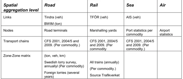
In Table 4.2 an overview over important data sources for goods transportation statistics is presented.

Table 4.2 Examples of data sources for validation data.

Spatial

aggregation level

Road Rail Sea Air

Links Tindra (veh)

BWIM (ton)

TFÖR (veh) AIS (veh)

Nodes Road terminals Marshalling yards Port statistics per commodity

Airport statistics

Transport chains CFS 2001, 2004/5 and 2009. (Per commodity.) CFS 2001, 2004/5 and 2009. (Per commodity CFS 2001, 2004/5 and 2009. (Per commodity.)

Zone-Zone matrix (ton, veh, km)

Swedish lorry survey, annuallyl (Per commodity)

Foreign lorries (several years)

All trains (annually) (Per commodity.)

Source Trafikverket

It seems to be possible to obtain vehicle flow data for individual links in the

SAMGODS network. For road traffic, there is a special database (Tindra) containing ÅDT11 data for NVDB12 links. In particular, the ÅDT data contains information about number of lorries (axle distance >3.3 m). A division into more detailed heavy vehicle categories might be possible. However, a difficulty when comparing Tindra data with SAMGODS data is that Tindra includes local (short distance) transports, which are normally not included in SAMGODS. In addition, a matching between the NVDB and SAMGODS networks must be performed in order to be able to transfer the ÅDT data from the NVDB to the SAMGODS netork. From Tindra it is also possible to obtain link flow data for a finer subclass13 of lorries. The data for the subclasses has less precision than for the aggregated total flows of lorries. A more serious problem for validation

11

ÅDT (“årsmedeldygnstrafik”) is the daily traffic flow on a link averaged over the whole year

12

NVDB: The national Swedish road database.

13

Link flow data for the following four subclasses of lorries is available: a) 2 axle trucks (tractors) with no trailer, b) 2 axle trucks (tractors) with a trailer, c) 3 axle trucks (tractors) without a trailer, d) 3 axle trucks (tractors) with a trailer, A possibility exists also to obtain data for 10 subclasses of lorries.

(21)

purposes is that these subclasses do not agree with the subclasses used in SAMGODS. It is necessary to perform a matching between the two sets of subclasses, an operation that can only be done by rather crude approximations.

Another database for road traffic is BWIM14, which contains total weights for vehicles passing bridges. However, it is not clear to what precision goods weight data can be deduced from the BWIM data. As for the Tindra data, it might also be difficult to use data on subclasses of lorries.

For goods transports on rail, it is possible to use a database based on actual departures of goods trains, TFÖR15. Unfortunately, it seems difficult to obtain commodity specific tonnes data for rail transports.

At sea, an automatic identification system (AIS) can be used to survey vessel

movements in real time. From this system it should be possible to deduce annual link flows. However, it is not possible to get any information about the amount of tonnes transported.

For individual nodes (terminals, marshalling yards and ports) it should be possible to obtain transfer data such as total weight of goods. Unfortunately, these data are often confidential.

For specific transport chains, the Swedish Commodity Flow Survey can be a useful data source.

For a zone-to-zone level, or with higher significance, a region-to-region level, the lorry survey provides information on traffic flow, tonkm and tonnes flow per commodity. Unfortunately, this survey only covers lorries registered in Sweden. The data can be supplemented to some extent with data for foreign lorries16.

14

BWIM: Bridge weigh in motion system.

15

TFÖR (“tågförseningsdatabas”) train delay database. It has been used in (Krüger, Vierth, & FakhraeiRoudsari, 2012)

16

See (Trafikanalys, 2012), (Vierth, Mellin, Hylén, Karlsson, Karlsson, & Johansson, Kartläggning av godstransporterna i Sverige, 2012)

(22)

5 Specifications for a validation database

In this section we propose a specification of the features of a validation database and define the capabilities and functionalities such a system should have. We also discuss a number of problems and difficulties that can be foreseen.

5.1 Summary of specifications

The requirements of the validation database are:

1. The database should include a structure that facilitates comparisons between model output data and validation data.

2. It must be possible to automatically import data from SAMGODS into the validation database and to transform data into the baseline data structure. 3. It should be possible to store several instances of model output data (typically

originating from different scenarios).

4. Likewise, it should be possible to store several instances of validation data (for example originating from different years).

5. The database must have a system for keeping track of “metadata”, i.e. data that describe a whole scenario or another large dataset, for instance, “year of

validity”, SAMGODS model version, commodity group classification systems, etc.

6. It should be possible not only to compare model output data with validation data, but also to compare two different sets of model output data. This could consist of results from different versions (updates) of the same model, as well as results from two different goods models.

7. If the aggregation levels of SAMGODS data and validation data differ, then the aggregation of data should be done automatically so that SAMGODS data and validation data could be compared.

8. If two datasets to be compared have differing classification systems for

commodity groups, then the validation database should manage to automatically translate these to a common classification system (provided that a translation key exists)

9. If validation data is missing for a specific year but is available for other years, then there should be a function in the validation database to impute data for the missing year.

10. It should be possible to compare not only “instant” data from a single model scenario, but also elasticities. Elasticities can be computed from two different SAMGODS scenarios (one basic and one slightly perturbed).

11. A system for protecting or handling confidential data must be available. 12. The large sets of output data from the validation (comparison of datasets) must

be handled somehow. Appropriate measures concisely describing the deviation between SAMGODS data and the validation data must be defined.

13. Missing values must be handled properly.

14. New comparison functions should be easy to implement.

15. The database should be able to discriminate between data of different levels of reliability. Alternatively, it should be possible to specify feasibility or

acceptance intervals for the data, i.e. minimum and maximum accepted values. 16. The data should be stored efficiently in the database.

(23)

Validation and model output data are stored in different modules (tables) in the database. We need to construct a system that can identify comparable datasets. It is important to safeguard consistency between validation data and model data.

5.2 Features and difficulties in more detail

5.2.1 A need for a uniform structure of data in the database

Although much of the output from a run of a particular scenario in SAMGODS is stored in a single .mdb file, the results are spread over a large number of different tables with diverse structures and formats, see Fig 5.1. Similarly, the validation data are also stored in many different formats. In a traditional cross table only a few independent variables can be displayed. In order to cover the many different combinations of independent variables, many different tables are used.

This diversity and inhomogeneity in data storage is very inconvenient when comparisons between model output and validation data are to be made. We have a matching problem: for each validation item, the corresponding model output item must be found whenever possible. Once each pair has been matched, comparisons can easily be done (by computing absolute and relative differences etc). There is need for a general, uniform data structure that is not likely to be changed in the future, and in which the matching problem can be conveniently solved.

Figure 5.1 The matching problem between model output data and validation data.

5.2.2 Differences in aggregation levels

The situation described in Fig 5.1 is further complicated by the fact that data, both model output data and validation data, may exist on many different aggregation levels. For example, tonkm (for a specific mode) can be available for each link in the network, for each OD pair, for each county, nationwide and even include international freight. Various aggregation levels exist not only in the spatial dimension (e.g. link level, regional, national and international level) but in other dimensions as well, such as transport modes, commodity groups and even time periods for more general models. The matching problem discussed in the previous section, also comprises any such differences in aggregation levels. In many cases, a specific quantity is available for both

(24)

validation data and model output data, but it differs in the aggregation level. For

example, model output data can be given in the form of directional flows on links, while validation data is available as the sum of the flows in both directions. Another example is that model output data can be given in terms of tons transported by individual

SAMGODS sea vessel types, while validation data may be given in terms of total tons for vehicle groups (such as container vehicles or total sea transport excluding ferries). Many other such examples can easily be found. The matching problem will not be satisfactorily solved unless a systematic procedure for filling in gaps has been constructed (imputation through aggregations) so that matching can be performed whenever the information in data allows for it.

5.2.3 Other discrepancies between validation and model output data

Besides differences in aggregation level there exist other types of differences between validation data and model output data that may complicate the matching.

One example is that validation data may occur only irregularly and might be missing for the specific time period. (For example, the Swedish commodity flow survey has been carried out every third year 2001; 2004/5, 2009.) The matching procedure requires that the time periods for both the validation and model output data exactly agree. A

possibility might then be to impute missing values by interpolation or extrapolation from other time periods.

Another possible type of discrepancy between validation and model output data is that the classification system for commodity groups may differ. The classification system of commodity groups in official transport statistics has been changed and updated a few times during the last decades. In about 2007, the NSTR-classification17 was replaced by the NST2007-classification18. In the different versions of the Swedish Commodity Flow survey, different classifications have been applied.

Another temporal variation is that the model itself (SAMGODS) appears in different versions. The output from one version may differ from another. It would be a great advantage if the validation database was able to administer output from different

SAMGODS versions. This would open for direct comparisons between the outputs from two different versions of the model and to check how model updates affect the results. 5.2.4 Elasticities for model outputdata

What makes elasticities special in the context of a validation database is that ordinary one-scenario model output data does not usually provide any elasticities. Instead, the original “base scenario” has to be slightly perturbed and the elasticities computed by taking differences between the two scenarios. A new scenario has to be created and run for each new perturbation to be studied, i.e. each new stimulus variable to be used. Since many different stimulus variables may be of interest, the number of scenarios that have to be run may become large. The computations of new scenarios have to be done by the model programme, i.e. outside the proper validation database. But the validation database must be able to host the results from the new scenarios.

17

NSTR = Nomenclature uniforme des marchandises pour les Statistiques de Transport, Revisée

18

(25)

Comparisons between elasticities from the literature and elasticities from SAMGODS results have to be made with caution, since circumstances between countries, or even regions, differ.

5.2.5 Special requirements for regional data?

In the current study, SAMGODS output data has been the special focus. However, the data structure in the validation database should be sufficiently general to also be able to host validation data for (future) regional or local goods models. Are there any special features in such models that have to be considered when designing the database? The SAMGODS output data can be compared to output data from two regional goods models: “the GORM model” for the Öresund region and NÄTRA19 for the Stockholm region. There is perhaps one notable difference between SAMGODS and NÄTRA (or other regional methods): while computations in SAMGODS are done for a given and constant time period (a year), the regional models take into account variations in travel time and level-of-service during a day. For instance, in NÄTRA, besides a 24 h period, three different time periods during the day may be considered: morning rush hour (7-8), normal daytime hours (9-15) and afternoon rush hour (15-17). The validation database must be able to also handle this kind of variations in time.

5.2.6 Variations in reliability

Different sources for statistical (and other) validation data have different levels of quality or reliability. In some cases, data has been obtained by means of a full survey of all the transports that are considered. In other cases, a statistical sampling has been done, resulting in an (estimated) uncertainty in the results. In yet other cases, validation data may have been obtained by crude estimates or computed by special models (most likely, elasticities have this precision).

In a validation database, it is a reasonable requirement to be able to somehow

distinguish between different levels of reliability. Data might be grouped into reliability classes. Each class may then be assigned a “reliability coefficient”, which can be used when evaluating the discrepancies between validation and model data.

19

NÄTRA (NÄringslivets TRAnsporter i Stockholms län) is a regional model for the vehicle movements of the economy in Stockholm County. It is based on a sample investigation of work places carried out in 1998. , The NÄTRA model has a traditional structure with OD matrix generation, traffic assignment, calibration with respect to traffic counts.

(26)

6 A proposed design for a validation database

In this section we propose a design for a validation database. In section 6.1, the overall structure of the database tables is described. In section 6.2, the important problem of aggregation is treated. In section 6.3 a series of other problems and issues are discussed. The handling of the very large amount of outputs from the comparisons/validations is the topic of section 6.4. Besides performing basic comparisons between model output data and validation data, there might also be other applications for the validation database. A few examples of extended functionalities are given in section 6.5. Finally, section 6.6 is devoted to the subject of data protection and security issues.

6.1 Structure of the validation database

6.1.1 A standard format

In section 5.1, we argued for the need for a uniform data structure. Instead of the situation visualized in Fig 5.1, it would be desirable to have all data stored in a uniform way as pictured in Fig 6.1. Each vertical line in a table represents a fixed field and each row should host exactly one (validation) value. The format of the two tables does not have to be identical, but there should exist a relation between them so that a matching between model output data and validation data can be made. The arrows in the figure represent importation of data from other databases (or tables). During the importation phase, data must be transformed into the uniform structure. We will call this data structure the standard format.

Figure 6.1 A uniform data structure (“standard format”) for both model output data and validation data.

6.1.2 The four main dimensions of data

Each row in the tables in Fig 6.1 contains only one “value field” (one item). The other fields (columns) in the table are used to uniquely determine or characterize what

quantity the value represents. We have to find a set of fields that can uniquely determine all output data from goods transportation models.

(27)

In order to achieve this, it can be observed that the model output data are essentially characterized by four main aspects (henceforth called dimensions): spatial extension,

time period, commodity type to be transported and vehicle type or loading unit of the

goods. A fifth dimension can also possibly be added: the unit of the quantity (i.e., tonkm, vehkm, etc). However, since “unit” has other properties than the ordinary dimensions (for example, no operations such as aggregations can act on the unit) we will not include “unit” among the dimensions.

For each dimension, several different aggregation levels (or classes) may be defined. In order to uniquely determine the value of the quantity, the aggregation level must also be specified.

6.1.3 Datasets

Both model and validation data are grouped into datasets. A dataset for the SAMGODS model typically consists of all the model data from one specific SAMGODS scenario. A dataset for validation typically consists of all validation data valid for one particular year. Datasets should be uniquely defined by an ID number. The ID numbers for the model output data should be independent of the ID numbers of the validation data. 6.1.4 The overall structure of the database

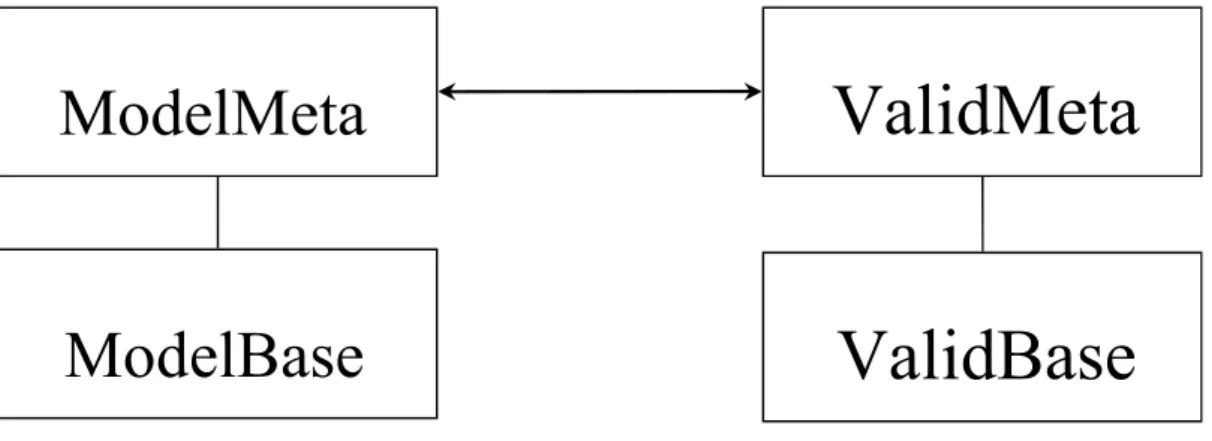
Some quantities are constant for all data items in a dataset. It is convenient to collect these in a metatable. In contrast, the detailed (varying) data in a dataset are collected in a base table. Different individual tables are used for model output data and validation data. The overall structure of the database is depicted in Fig 6.2. The database contains two metatables, one for model output data, ModelMeta, and one for validation data, ValidMeta. Each metatable consists of a list of all datasets in the database. Each dataset is uniquely determined by an ID number.

It seems reasonable to separate model output data from validation data. One reason for this is that they differ somewhat in structure. Another reason is that they differ in the way that they are imported and are therefore vulnerable to different types of risks for introducing errors. Moreover, they will (probably) differ a lot in size.

Figure 6.2 Tables in the validation database

ValidMeta

ModelBase

ModelMeta

(28)

6.1.5 The metatables

In Table 6.1, examples of fields (columns) in the metatables are listed. Each record in the metatable corresponds to a specific dataset, uniquely determined by ”IDdataset”. In order to connect the model output data with validation data, the user has to specify which IDdataset numbers in the ModelMeta and ValidMeta tables that correspond to each other (In this example the model dataset 134 corresponds to the validation dataset 725, see section 6.1.10). The field CommoditySys determines which classification system that is used in the base table for commodity groups. The field ModeSys

determines which notation is used in the base table for describing the individual modes. (ModeSys=”STAN” would mean that one-letter codes are used, while “Samgods” would mean HGV60, etc.). The field Table determines which of the SAMGODS and CUBE output tables the data item originates from.

Table 6.1 Possible structure of the metatables.

6.1.6 The base tables

In Table 6.2, examples of fields (columns) in the base tables are listed. Each dimension essentially corresponds to two fields: one field containing the aggregation level and the other containing the value. For instance, SpatAgg contains the spatial aggregation level (e.g “National”, “Regional”, “County”, “Municipal”, “Link”, “Node”) while SpatVal contains the specific spatial value for the given aggregation level. (For more

information on aggregation levels see section 6.2.) “IDdataset” is used for connecting with the corresponding item in the metatable (and hence also to the ValidBase table). “Value” contains the value for the current item (record). “Extra” is an additional space that is needed in some special cases (see 6.1.8). Additional fields, that describe data further, can be added, in particular to the ValidBase table. Here, two examples of additional fields are shown: Secret is a flag defining confidential data and Rely is an indicator for the reliability of the validation data (see section 6.1.9).

(In Tables 6.4 and 6.5 further examples of data items in a ModelBase table are shown.)

Field name Example Field name Example

IDdataset 134 IDdataset 725

NameOfDataset Basår2005 NameOfDataset År2005

TempUnit Year TempUnit Year

TimePeriod 2005 TimePeriod 2005

CommoditySys NSTR CommoditySys NST2007

ModeSys STAN ModeSys Samgods

ModelVersion 0.8

ModelScenario Bas2005

Table Report1

(29)

Table 6.2 The fields in the base table for model output data (ModelBase) and

validation data (ValidBase) respectively. SpatAgg=County means that the aggregation level is counties. SpatVal=5 means ”Östergötlands län”. TimeAgg and TimeVal can be excluded if TempUnit and TimePeriod are included in the metatables.

Note that model output data from different SAMGODS scenarios (or even different goods models) can (should) be stored in the same ModelBase table in a format similar to the one used in the ValidBase table.

The price to be paid for this conformity is that it requires more storage than a more compact data structure (see the example in section 3.2.3). Although the advantages in simplicity prevail, some complications may force us to deviate from this simplistic ideal (see section 6.6).

For reasons of storage size, one might consider further separating the table ModelBase into two tables: one containing aggregated data and the other disaggregated data, typically matrices or flows on network links.

6.1.7 The unit field

The unit field in Table 6.2 is not regarded as a dimension since it can’t hold any aggregation levels. Unit is simply a qualifier to distinguish different variables. (This means that no aggregations will be done over the unit field.) As with aggregation classes, we are not restricted to the “classical” units (such as tonkm, vehkm, tonne, etc.) but may arbitrarily invent new ones needed to describe the data. The only important matter is that the same system or terminology must be used for the model output data and the validation data.

For example, any effect unit can be specified in the unit field: kWh, CO2[g], #injured, noise[dB], or whatever. Any type of cost associated with the effects can also be specified: delay[SEK], NOx[SEK], etc.

Field name Example Field name Example

IDdataset 134 IDdataset 725

Value 1.234 Value 1.131

Unit TonKm Unit TonKm

SpatAgg County SpatAgg County

SpatVal 5 SpatVal 5

SpatVal2 - SpatVal2

-CommodAgg Samgods CommodAgg Samgods

CommodVal 25 CommodVal 25

ModeAgg Main ModeAgg Main

ModeVal Rail ModeVal Rail

TimeAgg Year TimeAgg Year

TimeVal 2005 TimeVal 2005

Extra - Extra

-Secret 0

Rely 3

(30)

PWC matrices20 have spatial properties that are rather similar to those of ordinary OD matrices. It is natural to use the same spatial aggregation class for both of them (MATRIX). Instead, they might be distinguished by different units, e.g., PWC_tonne, OD_tonne, etc.

(Alternatively, different spatial aggregation classes could be defined for the PWC and OD matrices, but it seems less natural to do so.)

In order to avoid confusion and to simplify the interpretation of results, it is desirable to standardize the various classes that are used in the unit field.

6.1.8 The extra field sometimes needed to uniquely specify a particular quantity

In some circumstances, the four dimensions (+ the unit field) are insufficient to uniquely describe a particular quantity. For example, one may want to distinguish between loaded and empty vehicles, or one might consider only goods carried by containers. Another possibility is that it might be desirable to separate PWC matrices from OD matrices, as discussed in the previous section.

The extra information needed to uniquely describe a data item in these cases21, could be stored in the Extra field in Table 6.2.

6.1.9 Some additional information fields that contain information on the type and quality of validation data

Besides the fields described above which uniquely determine a specific item, it might be appropriate to introduce some additional fields that contain useful information about the item. These kinds of additional fields will primarily be useful when dealing with

statistical data. The extra information is not needed in the matching process, but may be useful in later steps to facilitate the interpretation or evaluation of the results. For example, the fields Rely and Secret in Table 6.2, may contain information about the reliability of the statistical data or whether the current item is confidential or not. Any number of additional fields of this kind may be introduced without essentially affecting the structure of the database. Further examples may include a reference to the source of the statistical data or some other descriptions. In particular, for links in a network which (spatially) are described by rather anonymous node numbers, it might be appropriate to introduce a more mnemonic description (e.g. “Svinesund” for one of the border crossings to Norway). This can be useful in the evaluation step when searching for a particular item. Another example might be a description of the source from which the validation data has been obtained, or a contact person.

20

PWC matrices are normally regarded as input data to the SAMGODS model and are therefore maybe not a good example. Still, the point here is to illustrate that there might exist different types of matrices in model output data.

21

Alternatively, this extra information can be stored elsewhere. For example, the loaded or empty cases might be described by adding a suffix to the unit (e.g. VehKm_L, VehKm_E) as is done in SAMGODS output data. We believe, however, that it is preferable to keep the units clean and to store the

loaded/empty information elsewhere.

The loaded/empty case is perhaps of such importance that one might consider to introduce a special field (or dimension) for it. The aggregation operation (L+E) might then be applied.

(31)

6.1.10 Matching validation and model output data

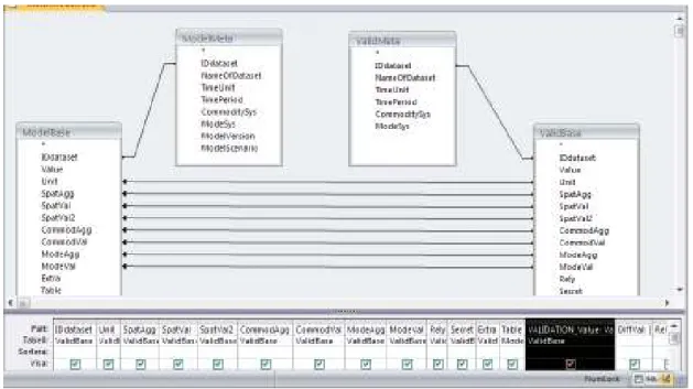
The uniform structure of the database tables described in the previous section makes matching and comparison between model output data and validation data an almost trivial task. In the simplest case, where the metadata agree (same year, same commodity group classification system, etc), the basic computations can be done with one single SQL statement22. The SQL statement can be illustrated graphically in terms of an MS Access query interface, see Fig 6.3:

Figure 6.3 The matching between validation data graphically illustrated as an MS Access query. Simplified case when the metadata agree.

The SQL statement selects all the records in the table ValidBase having the same dataset ID as the selected dataset in ValidMeta, and merges23 them with the

corresponding selected records in ModelBase. The absolute and relative differences are also computed and all relevant values are written to a new database table: “Results”. We can distinguish three different types of “strengths” for the matching between ValidBase and ModelBase:

1. Only keep those records that match each other exactly (normal case)

22

SELECT ValidBase.IDdataset, ValidBase.Unit, ValidBase.SpatAgg, ValidBase.SpatVal, ValidBase.SpatVal2,

ValidBase.CommodAgg, ValidBase.CommodValProdGroup, ValidBase.ModeAgg, ValidBase.ModeVal, ModelBase.Value AS SAMGODS_Value, [Modelbase].[Value]-[ValidBase].[Value] AS DiffVal, [Diffval]/[ValidBase].[Value] AS RelVal, ValidBase.Rely, ValidBase.Secret, ValidBase.Extra, ModelBase.Table, ValidBase.Value AS VALIDATION_Value, ValidBase.Description, ValidBase.Direction, ValidBase.Source, ValidBase.FilterCode INTO Results

FROM ValidBase LEFT JOIN ModelBase ON (ValidBase.Mode = ModelBase.ModeVal) AND (ValidBase.ModeAgg = ModelBase.ModeAgg) AND (ValidBase.CommodVal = ModelBase.CommodVal) AND (ValidBase.CommodAgg =

ModelBase.CommodAgg) AND (ValidBase.SpatVal2 = ModelBase.SpatVal2) AND (ValidBase.SpatVal = ModelBase.SpatVal) AND (ValidBase.SpatAgg = ModelBase.SpatAgg) AND (ValidBase.Unit = ModelBase.Unit) AND (ValidBase.IDdataset = ModelBase.IDdataset)

23

Note that the coupling between ModelMeta and ValidMeta tables is done by the user interface where the user specifies the IDdataset numbers for each table.

(32)

2. Keep all elements in ValidBase and those elements in ModelBase that matches them

3. Keep all elements in ModelBase and those elements in ValidBase that match them

The second type will include all values from ValidBase, even those lacking a matching value in ModelBase. In these cases, the ModelBase values will be represented by an empty cell and differences between the validation and model output data items are not defined. Displaying these cases may still be very useful for finding the reason why the matching failed. The third type is analogous to the second, but instead, the validation data may be represented by an empty space. This case is useful for revealing what kind of validation data is missing.

In Fig. 6.3, the arrow heads reveal that in this particular case, a type 2 matching is made. When running the validation database, users will be given the option to select the

preferred type of matching24.

It is important to note that the matching procedure (the SQL statement) is independent of the specific data items in the database. Thus, one may introduce new aggregation classes, new units, or any other data into the database without needing to modify the SQL statement. The only thing that matters (for the matching procedure) is that the model output data and the validation data should correspond (be consistent). In section 6.6, some complications that may occur are discussed, but essentially it should be possible to maintain this simple structure.

Matching the output from two different model versions can be done in a similar way and only a slight modification of the SQL statement is needed. Further, one might consider including a function for a similar comparison between all validation data originating from different time periods.

6.2 The aggregation problem

As was seen in section 5.2.2, for a successful matching it is necessary that the validation data and model output data have the same aggregation level. There is need for a

systematic procedure to “fill any gaps” by aggregating from one level to another. This problem is addressed here. We start by giving an overview of the aggregation classes. 6.2.1 Aggregation levels (or classes)

Both model output data and validation data come in a variety of different aggregation levels. It may also be useful to introduce new aggregation levels. It is sometimes more appropriate to speak of aggregation classes rather than levels, since one cannot always distinguish a specific level for the aggregations. We use both terms in this report as the distinction is not important.

24 The Extra field might possibly be used for an alternative way to vary the “strength” of the matching. The Extra field might contain specifics that are less important than in other fields. I.e., the distinction between different cases in the Extra field might be less accentuated. (For instance, in case we only have statistical data for Container transport, we might still want to be able to compare it with Container+Non-container transports.) A possibility may then be to give the user the option to choose whether the Extra field should be included among the fields that should be matched. This would allow for a more relaxed matching in cases where otherwise the matching would be too restrictive.

(33)

We will distinguish between two types of aggregation classes: basic aggregations and

special aggregations. The basic aggregations naturally occur in the original dataset,

while special aggregations are new aggregation types that are introduced for special purposes. The special aggregation classes are always computed from other aggregation classes. Usually a key table is used for defining a special aggregation class. The key table can be modified by the user if so desired.

We will give examples of basic aggregation classes and special aggregation classes in the following subsections.

6.2.2 Basic aggregation classes

In Table 6.3, a list of all basic aggregation classes from the SAMGODS output data is shown. Each aggregation class has a permitted set of values. Each permitted value may be a numeric number, a pair of numeric numbers, a text string or a pair of text strings. From other goods models (regional, local...) additional basic aggregation classes may arise. For instance, for a local goods model it may be natural to define the spatial aggregation class SAMS, corresponding to local SAMS areas25 (its set of values would be the SAMS area numbers).

There might be more appropriate names for the aggregation classes in Table 6.3. For example, it is perhaps better to call the aggregation class “Detail” in the mode dimension “VehicleType”. One might possibly add an aggregation class,

“International”, instead of using the “INT” value for the “National” aggregation level.

NOTE: It is important to standardize these notations! The names used in Table 6.3 are

not the final suggestions!

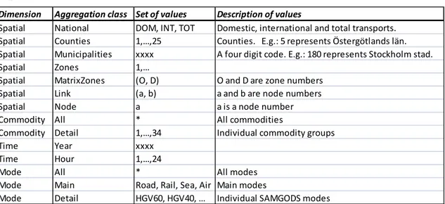
Table 6.3 Basic aggregation classes for SAMGODS output data. A ‘*’ represents an empty value, i.e. the content is not relevant.

In Table 6.4, it is shown how various items belonging to different basic aggregation levels may be represented in the ModelBase table. The spatial dimension needs two value fields in order to be able to represent quantities such as Link, Matrix and ZoneX.

25

SAMS: Small Area Market System.

Dimension Aggregation class Set of values Description of values

Spatial National DOM, INT, TOT Domestic, international and total transports.

Spatial Counties 1,…,25 Counties. E.g.: 5 represents Östergötlands län.

Spatial Municipalities xxxx A four digit code. E.g.: 180 represents Stockholm stad.

Spatial Zones 1,…

Spatial MatrixZones (O, D) O and D are zone numbers

Spatial Link (a, b) a and b are node numbers

Spatial Node a a is a node number

Commodity All * All commodities

Commodity Detail 1,…,34 Individual commodity groups

Time Year xxxx

Time Hour 1,…,24

Mode All * All modes

Mode Main Road, Rail, Sea, Air Main modes

(34)

Therefore both SpatVal and SpatVal2 are needed. Similarly, one might also need two value fields for the the modes dimension, if for instance, it should be possible to represent transfers from one mode to another in a node.

Note that the Time dimension has been excluded in Table 6.4. For SAMGODS data, the time period is always one year and it is sufficient to specify this in the metatable. For data with varying time periods, TimeAgg and TimeVal should be included in the ModelBase table.

Table 6.4 ModelBase table contaning (a few) items belonging to various basic aggregation levels. A ‘*’ represents an empty value, i.e. the content is not relevant.

6.2.3 Examples of special aggregation classes

It is very useful to supplement the basic aggregation classes with additional classes for different purposes. New special aggregation classes can be invented arbitrarily. The only requirement is that they fit into the general pattern of ModelBase and ValidBase. Each special aggregation class must belong to one of the four dimensions (spatial, temporal, commodity group or vehicle group). For spatial aggregation classes, each class must be uniquely determined by at most two parameters. For other dimensions, each class must be uniquely determined by one single parameter (with the possible exception of Modes).

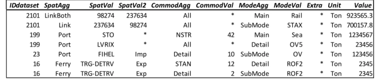
In Table 6.5, examples of items belonging to special aggregation classes are shown. Each of the new classes are described below.

Table 6.5 ModelBase table containing items belonging to various special aggregation classes. Note the difference between LinkBoth and (the basic aggregation class) Link.

LinkBoth:

The purpose of this special aggregation class is to describe the total flow (or similar quantities) on a link, i.e. the sum of the flows in both directions. The basic aggregation class “Link” represents one-directional flows only. Thus, aggregating from Link to LinkBoth involves a summation over the two directions. Link is specified by the node numbers for the start and end nodes (see SpatVal and SpatVal2 in Table 6.5). The same node numbers can be used to specify an element in Linkboth, but since LinkBoth does not depend on the direction, the forward and backward links have to be treated as

IDdataset SpatAgg SpatVal SpatVal2 CommodAgg CommodVal ModeAgg ModeVal Extra Unit Value

2101 National DOM * Detail 23 Main Rail * Tonkm 923565.3

2101 Link 237634 98274 All * Detail HGV40 * Ton 7157.8

34 Matrix 256 254 Detail 2 All * * Ton 651.3

2101 ZoneX 345 Export Detail 29 All * * Ton 56.2

34 County 5 * All * Detail KOMBI * NV 370

4 Zone 198 * Detail 34 Main Road * Vehkm 23.1

IDdataset SpatAgg SpatVal SpatVal2 CommodAgg CommodVal ModeAgg ModeVal Extra Unit Value

2101 LinkBoth 98274 237634 All * Main Rail * Ton 923565.3

2101 Link 237634 98274 All * SubMode STAX * Ton 700157.8

199 Port STO * NSTR 42 Main Sea * Ton 1234567

199 Port LVRIX * All * Detail OV5 * Ton 23456

23 Port FIHEL Imp Detail 10 SubMode OV * Ton 123456

16 Ferry TRG-DETRV Exp STAN 12 Detail ROF2 * Ton 2345

(35)

identical. For LinkBoth, this can be formally achieved by requiring that the node number in SpatVal is always less than the node number in SpatVal2.

LinkBoth is an aggregation class that naturally belongs to the spatial dimension. Port:

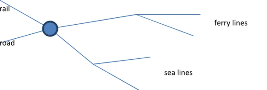
In SAMGODS, a port is represented by a node. However, the goods flow through the port is not represented by a node attribute but instead by the flows on the adjacent links, see Fig. 6.4.

Figure 6.4 The representation of a port in SAMGODS. The goods flow through the port can be described by the flows through the adjacent links.

In order to compute the total goods flow through the port, a summation of flows on the adjacent links must be done (ferry lines and other sea lines are usually represented by different links from the port). This can be considered in abstract terms as an aggregation of links. Thus, we introduce the special aggregation class, Port, by considering it as an aggregation of elements in the basic aggregation class Link. Port is an aggregation class that naturally belongs to the spatial dimension.

In order to be able to represent the ports in tables ModelBase and Valid Base, it is appropriate to introduce a special code for each port. We suggest to use the coding system by UN/LOCODE26. Each port has a five letter code, CCPPP, where CC represents the country code and PPP is a three letter code for the port. The code in the SpatVal field in Table 6.5, DETRV, denotes Travemünde. For Swedish ports it may be appropriate to omit the country code.

The definition of the ports in terms of links is specified in a special key table. The key table is used when aggregating from Link to Port. Thus, any details in the definition of the port are described in the key table instead of ModelBase and ValidBase. All ports are defined in one and the same key table.

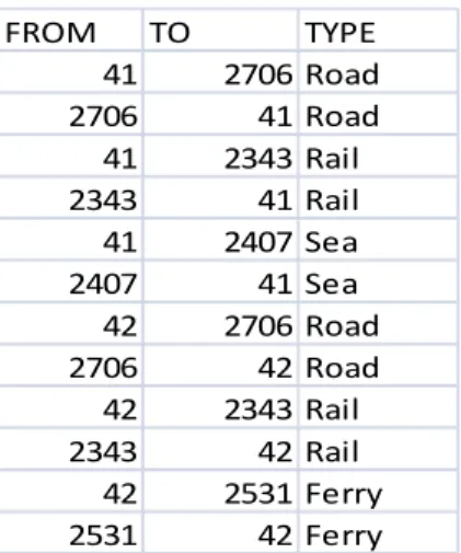
In Table 6.6 an example how a port (Stockholm Värtan) is represented in a key table is shown. There are 12 different links involved. However, not all of them should be included when aggregating the sea transports to/from the port. The links of type Road and Rail should only be included if land transports to/from the port are considered.

26

United nations Code for Trade and Transport Locations. It is a geographic coding system developed by the UNECE (United Nations Economic Commission for Europe) for more than 40,000 locations

worldwide. rail

road

ferry lines

(36)

Table 6.6 Representation of the port Stockholm Värtan as a set of links in a key table. The fields FROM and TO contain node numbers.

A variety of similar special aggregation classes can be defined, some examples: • PortIn: aggregation of all (adjacent) links directed from the sea towards the port

• PortOut: aggregation of all (adjacent) links directed towards the sea from the port

• PortRoad: aggregation of all road links connected to the port

• PortRail: aggregation of all rail links connected to the port

• PortFerry: aggregation of all ferry links connected to the port

Alternatively, and maybe better, we can use one and the same aggregation class, Port, for all of these cases, but instead distinguish them by different qualifiers in the field SpatVal2: In, Out, Road, Rail and Ferry. For an example, see item “Port FIHEL” in Table 6.5.

Ferry:

Just as with ports, it is useful to define the special aggregation class, Ferry, and to introduce a code for each ferry line. We may use the UN/LOCODE coding system for ports to also define codes for ferry lines. For example, the string NYN-PLGDN may represent the ferry line Nynäshamn-Gdansk. As a convention, we always set the

Swedish port first in the string. (For ferry lines within Sweden we set the mainland port first, OSK-VBY.) The ferry code is put into the SpatVal field, see Table 6.5. The direction of the transportation (Imp, Exp or Both) can be put into the SpatVal2 field. Similarly to the Port class, the definition of the ferry lines in terms of links is specified in a special key table.

A difficulty concerning how to properly represent a ferry line in terms of SAMGODS links arises. In Fig 6.5, a typical situation is shown. The ferry line is made up of a chain of links (having Mode=4). If more than one ferry line starts from a port, the first (or the first few links) is shared among the ferry lines (e.g. Visby and Gdansk).

In the validation database, there are two natural alternatives: either the ferry line is represented by all the links in the chain or it is represented by only one of the links. The first case is convenient for computing tonkm or vehkm, while the second option is

FROM TO TYPE 41 2706 Road 2706 41 Road 41 2343 Rail 2343 41 Rail 41 2407 Sea 2407 41 Sea 42 2706 Road 2706 42 Road 42 2343 Rail 2343 42 Rail 42 2531 Ferry 2531 42 Ferry