Reservoir Computing Approach for Network Intrusion Detection

Västerås, Sweden

Thesis for the Degree of Bachelor of Science in

Computer Science 15.0 credits

RESERVOIR COMPUTING APPROACH

FOR NETWORK INTRUSION

DETECTION

Casper Andersson

can18010@student.mdh.se

Examiner: Sasikumar Punnekkat

Mälardalen University, Västerås, Sweden

Supervisor(s): Miguel León Ortiz

Mälardalen University, Västerås, Sweden

Abstract

Identifying intrusions in computer networks is important to be able to protect the network. The network is the entry point that attackers use in an attempt to gain access to valuable information from a company or organization or to simply destroy digital property. There exist many good methods already but there is always room for improvement. This thesis proposes to use reservoir computing as a feature extractor on network traffic data as a time series to train machine learning models for anomaly detection. The models used in this thesis are neural network, support vector machine, and linear discriminant analysis. The performance is measured in terms of detection rate, false alarm rate, and overall accuracy of the identification of attacks in the test data. The results show that the neural network generally improved with the use of a reservoir network. Support vector machine wasn’t hugely affected by the reservoir. Linear discriminant analysis always got worse performance. Overall, the time aspect of the reservoir didn’t have a huge effect. The performance of my experiments is inferior to those of previous works, but it might perform better if a separate feature selection or extraction is done first. Extracting a sequence to a single vector and determining if it contained any attacks worked very well when the sequences contained several attacks, otherwise not so well.

Contents

1. Introduction 1

2. Background 2

2.1. Time series . . . 2

2.2. Intrusion Detection . . . 2

2.3. Artificial Intelligence and Neural Networks . . . 3

2.3.1. Classification . . . 4

2.4. Recurrent Neural Networks . . . 4

2.5. Reservoir Computing . . . 5 2.6. Feature Extraction . . . 6 3. Related Works 7 4. Problem formulation 9 5. Method 10 6. Ethical Considerations 11 7. Work process and implementation 12 7.1. Datasets . . . 12

7.2. Preprocessing . . . 12

7.3. Implementation . . . 13

7.4. Performing the experiment . . . 13

8. Results 14 8.1. Many-to-many experiments . . . 14 8.2. Many-to-one experiments . . . 16 9. Discussion 17 10.Conclusion 19 11.Future Work 20 References 21

List of Tables

1 Amount of entries in datasets and how many % of those are attacks. . . 12

2 NSL-KDD. ˙E ˙S ˙N. Reservoir size: 100. Connectivity: 20% . . . 14

3 KDD99. ˙E ˙S ˙N. Reservoir size: 100. Connectivity: 20%. . . 15

4 MGAM. ˙E ˙S ˙N. Reservoir size: 100. Connectivity: 20%. . . 15

5 Many-to-many. No time aspect. Reservoir size: 100. Connectivity: 20%. . . 15

6 KDD99. ESNx. Reservoir size: 100. Connectivity: 5%. . . 16

Acronyms

ANN Artificial Neural Network DR Detection Rate

ESN Echo State Network. A type of reservoir computing FAR False Alarm Rate

IDS Intrusion Detection System

KDD99 Dataset from KDD cup in 1999 LDA Linear Discriminant Analysis

LSTM-RNN Long Short-Term Memory RNN MGAM Dataset from Alkasassbeh et al. NN Neural Network

NSL-KDD Modified version of KDD99 RC Reservoir Computing

RNN Recurrent Neural Network SVM Support Vector Machine

1.

Introduction

The internet is becoming a more and more integral part of our lives. As the internet has grown, illegal activities have also followed the digitalization. Attacks on networks are a big concern for many big companies and organizations[2]. They often have valuable data that the attackers may want to access, data that is often of monetary value either directly or indirectly. It could be user information that can be sold for money or emails and passwords that can be used in an attempt to access the accounts of that person. Trade secrets can also be very valuable. It could also be that they simply want to cause damage or deny access for others, pure vandalism.

For companies to protect themselves against intrusions they employ automated systems that identifies and blocks malicious traffic. These systems are called Intrusion Detection Systems (IDS), or Intrusion Prevention Systems if they also take action against it. An IDS simply classifies the traffic as to whether it is malicious, although the terms are often used interchangeably today. The main issue here is the detection part. Many studies have been performed in an attempt to improve the detection accuracy of these systems. Some of these are Fu et al. [3], Shrivas and Dewangan [4], Alkasassbeh et al. [1]. They reached accuracies of around 97–99% in classification of attacks in network traffic on their respective datasets.

I wanted to try creating an IDS using a reservoir network, to utilize the time aspect of the reservoir to detect when abnormal traffic is encountered. I have compared different classifiers, with and without preprocessing the data with the reservoir, to determine which worked best and if the reservoir was useful as a feature extractor in classification of network traffic.

Similar to Fu et al. [3], I chose to use a time-based neural network. In this thesis, I have applied a reservoir network, a variation of recurrent neural networks, in an attempt to classify network attacks. Network traffic is a time series since a network continuously receives traffic over extended periods of time. The inputs go through the reservoir network and then they go to another classifier, as the reservoir network itself isn’t trained. I tested intrusion detection with a Neural Network (NN), Support Vector Machine (SVM), and Linear Discriminant Analysis (LDA). I did this in two variations. One where the reservoir network takes input and outputs a new vector on each timestep, the state is updated with each input. Then I compared the classifiers to being trained on the raw input versus being trained on the reservoir’s outputs. I also tried taking a shorter sequence of inputs and running them through the reservoir to get a single final output. The final output represents the whole sequence. Then I trained the classifiers in an attempt to find if the sequences contained any attacks.

The NN generally performed better with the reservoir than without. The SVM performed better sometimes and worse sometimes. The LDA performed worse with the reservoir, most likely because the reservoir output does not fulfill the requirements that LDA has to create reliable predictions. Accuracy could probably be improved by doing additional feature selection/extraction beforehand. The results of taking a whole sequence and reducing it to a single vector through the reservoir showed to be very effective when there is a clear difference and attacks are plentiful. When a single attack occurs in a sequence of 9 other normal traffic inputs the difference of the attack is evened out by all the normal traffic.

Section 2. covers the prerequisites needed to understand my work. Section 3. explains some previous works in intrusion detection and time series classification. Section 4. explains the purpose of this thesis. Section 5. explains the method used to create this thesis. Section 6. talks about the ethical considerations regarding this research. Section 7. describes in detail how the experiments were performed. Section 8. lists the results from the experiment. Section 9. discusses the results, why the results are as they are and what it means. Section 10. contains the conclusion of my research and explains what this thesis has achieved.

2.

Background

This section contains the prerequisite knowledge for my research. It covers the type of data used and the purpose. It explains what, in simple terms, artificial intelligence is along with some methods of machine learning and the way they will be used in this thesis, classification. You will learn how different types of neural networks work, including feed-forward neural networks, recurrent neural networks, and reservoir networks.

2.1.

Time series

Time series data is data values taken at discrete points in time[5]. The actual timestamp of the data entries is not relevant in time series, only the order in which they appear. A data entry will usually have some form of relation to the previous values, with the most recent ones being the most influential. Though the timestamp doesn’t matter the intervals between the data entries still need to be taken into account when gathering the data. Too long intervals and there will be no useful information to extract from it. For example, looking at the weather once a week will hardly tell you anything about the weather next week. Looking at the weather every hour will tell you a lot about how it has changed throughout the day, and you can make a decent guess as to how it will look in the next hour. Grey clouds slowly moving towards you throughout the day could indicate there is a chance for rain in the next hour. It is important to base it on multiple data points. Only looking once will not tell you if the clouds are moving towards or away from you. Having a computer process and analyze time series data is helpful in many areas with predicting the future or identifying certain behavior, for example, detecting anomalies.

An anomaly is a change to an unexpected value of the data. It could have changed to something that is not possible or something that indicates problems. What classifies as an anomaly may depend on what the data previously looked like. If the data follows a certain pattern then any big deviations from that pattern are anomalies. For example, on a web server, it is expected to see a lot of HTTP requests, but many SSH requests in a short span may indicate someone is trying to guess the password.

2.2.

Intrusion Detection

Identifying these network attacks is called intrusion detection[6]. A system or program that does this is called Intrusion Detection System (IDS) and does it by automatically analyzing the incoming requests in the network. There are three common ways of doing this.

1. Signature-based detection. It matches the incoming requests against patterns of already known events. This is effective in protecting against known attacks, but can completely miss unknown attacks if they don’t match any previously known attacks. Signature-based detection also requires manual labor to keep the list of signatures up to date when new attacks become popular.

2. Anomaly detection. As mentioned in the previous section it detects when the data deviates from the normal activities. This can be done with unsupervised machine learning by teaching the model what normal behavior is. Normal behavior is obtained by monitoring data over some time period where no attacks have occurred. The normal behavior profile is then used as a baseline when analyzing incoming network traffic. Using supervised machine learning this can be done by exposing the model to both normal traffic and malicious traffic. Anomaly detection can be good at detecting previously unknown attacks, but the accuracy may not be as good over time as what is defined as an anomaly can change.

3. Stateful protocol analysis. This works similar to anomaly detection, but instead of working on the previous behavior of the current network it uses generic predetermined profiles of ‘normal activity’. These profiles are based on protocol standards and contain information on what non-malicious requests typically look like. This method is very resource expensive compared to the other two.

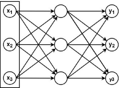
Figure 1: A neural network (NN) with one hidden layer

Each of these three methods has different pros and cons, and there exist many different al-gorithms that use these methods. Some are based on time series. On top of detection, there also exists Intrusion Prevention Systems, systems that intercept and block these malicious requests.

2.3.

Artificial Intelligence and Neural Networks

Artificial Intelligence is a computer program that makes intelligent decisions[7]. This can be split into four main categories. Thinking humanly, acting humanly, thinking rationally, and acting rationally. The two first aim to represent how we humans think and act. The latter two aim to reach the ideal performance, the best possible given the circumstances. Humans don’t always think rationally, and we surely don’t always make the best choices. Although what we humans can do is interpret information and make an educated guess based on previous experiences.

A neuron is a cell designed to transmit signals to other cells[7]. A neural network is a network of neurons connected by synapses that make up our brain. An Artificial Neural Network (from here on they will be referred to as just Neural Networks or NN) is a simple virtual version of a real brain in the sense that they have a network of virtual neurons that send signals to each other. When one neuron is triggered it sends a signal to all the connected neurons, which in turn may trigger those neurons to send their signals. When the signals come into a neuron the values of the signals are summed up and then run through the perceptron. To decide if the neuron should fire an activation function is used, also known as a perceptron. If the output value of the perceptron is 0 then it is equivalent to not sending a signal. This signal is then modified by a bias weight that determines how much a specific connection matters. The weights are typically randomized at the start. To start triggering the neurons in a NN some numerical input is sent to them. The input is then run through the perceptrons which will start the chain reaction of signals.

Feed-forward NNs are the simplest model[7]. They consist of two or more layers of neurons, wherein each layer all neurons from the previous layer are connected (one-way connection) to all neurons of the current layer, where the input layer is the first layer and the output layer is the last. The signals all go in the same direction and it’s easy to compute one layer at a time. There is no state and the whole network essentially acts like a function. To improve the NN the bias weights are trained using backpropagation. It calculates the error, how far it was from the right answer, and adjusts the weights accordingly to make the output more correct for future inputs. This is what puts neural networks in the ‘acting humanly’ category. It can learn from its mistakes and possibly make a better guess next time. Figure 1 shows a neural network with 3 layers, the input layer, one hidden layer, and the output layer. The arrows indicate the connections. Each arrow has a weight associated with it.

2.3.1. Classification

Data classification is the act of placing some data in the right category[8]. Classification algorithms are a type of supervised machine learning where the model trains on labeled data to learn what input features and values are more likely to be associated with which output category. For ex-ample, in a network, an attack can be labeled as such, while any other activity is labeled normal. By training on such data, the algorithm can learn to differentiate between normal activity and attacks on the network based on what the request looks like. Some common methods for this are probabilistic methods, Support Vector Machine methods, and neural networks.

Probabilistic models are statistical models that infer the probability that an input is in one class, based on what previous inputs looked like[8]. If an input looks the same as a previous one then it is very likely that is in the same category. They usually give an output with values between 0 and 1 to represent how likely it is that the input belongs to the different classes. One example of a probabilistic classifier is logistic regression. It is commonly used on yes/no questions to give a single percentage of how likely the answer is yes. If 1 indicates ‘yes’ then a value of 0.25 would indicate that it’s more likely to be ‘no’ because it’s closer to 0. You can of course name yes/no whatever you want, but it operates in the way that one option being more likely means the other one is less likely.

Logistic Regression can be extended to handle several output classes, but this is rarely done[9]. Instead, Linear Discriminant Analysis (LDA) can be used. For example, an IDS could have just a single output if there is an attack, yes or no. Or it could have one output for each type of attack and output how likely it is to be each attack. This is what LDA does. And to get a final prediction by looking at which class has the highest probability. LDA follows the assumption that the input features follow Gaussian distribution and that each feature has about the same variance. If this is not the case then performance may be bad.

Support Vector Machines (SVM) is a model for binary classification only, meaning there are only two options to choose from[8]. It works by separating the data points with hyperplanes in the dimension of the data. For example, if the data is in two dimensions (eg. coordinates in a grid) then they can be completely separated by lines. If the data is three-dimensional then it needs to be separated by a plane. The definition of a hyperplane is a space in one dimension less than that of the data. In cases where data can’t be linearly separated soft-margin methods can be used.

Neural networks, as previously explained, use backpropagation to train by adjusting the weights of the connections[8]. To apply this to a classification problem we can set the output layer to have as many neurons as there are categories to classify as. Then, using a softmax function as the activation function on the last layer, the output neurons will contain the probabilities of the input being each category. If it is binary classification we can just use a single neuron, where closer to 0 indicates it is group 1 and closer to 1 indicates group 2, and use an activation function that gives a value in that range.

2.4.

Recurrent Neural Networks

A Recurrent Neural Network (RNN) is a type of neural network where the neurons can have loops to themselves, hence the name recurrent[10]. It typically uses a layer structure like feed-forward NNs, but a node may have an edge to itself (see Figure 2). When a neuron outputs to a loop edge that output will be used as input for the next computation, which is initially zero. This opens up the possibility for the network to be a dynamic system. An RNN has a hidden internal state, the recursive outputs, where it can remember information about previous inputs by sending some information to itself the next computation. This makes it ideal for processing time series. RNNs typically use gradient descent to optimize the weights of the network, although it can be computationally expensive for large networks and it may degenerate over time to the point where it’s no longer useful.

A traditional feed-forward NN typically uses a one-to-one mapping from input to output[11]. An RNN can also do many, many-to-one, and many-to-many mappings. Using a one-to-many relation the network can take a single input and based on that produce a sequence of outputs, where each output is fed as input for the next computation. This lets the RNN create a possible sequence following the first input. For example, it might take the state of the weather right now as input and then output how the weather could change within the near future. For each prediction

Figure 2: A recurrent neural network (RNN) with loops on the hidden layer.

it makes it uses that prediction as a base for the next prediction along with the previous ones. Although, given only one input there is a lot of room for wrong predictions.

A many-to-one mapping would instead take in a sequence of input to produce what comes next in the sequence[11]. An example of this would be word autocompletion one letter forward. It takes the current word you are writing and suggests a possible next letter to type. The weather example in Section 2.1. is also an example of this. Instead of predicting it can also use that one output to tell some information about the sequence. These methods can also be combined. By combining many-to-one with one-to-many it becomes a network that first takes a sequence of inputs and then produces a sequence of outputs, ie. a sequence-to-sequence mapping. This could be used to create a full autocomplete by taking the word you have written so far as input and outputting a possible sequence to follow it.

Many-to-many differs from many-to-one + one-to-many in that every computation will have new input and output[11]. This could be used to monitor some machine that outputs sensor data at regular intervals, to find when it starts showing weird behavior, ie. anomaly detection. At every new input data, it decides whether it is an anomaly, based on how it relates to the previous inputs[10]. It takes in a time series data as input and outputs a time series data with the result.

2.5.

Reservoir Computing

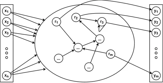
The idea of Reservoir Computing (RC) originated in the models Echo State Network (ESN) and Liquid State Machine, which developed independently of each other around the same time, and later came to include the Backpropagation-Decorrelation learning rule[10]. A reservoir network is a type of RNN where the network consists of a set of input neurons, a set of hidden neurons which is called the reservoir, and a set of output neurons. Every input neuron is connected to all neurons in the reservoir, and the output neurons have a one-to-one connection to the hidden neurons (bijective mapping). What makes RC networks special is that the neurons inside the reservoir can be connected to each other and the weights inside the reservoir cannot be trained. The reservoir only exists to hold the state, the memory of the network. The weights of the reservoir neurons are initialized to random values at the start and cannot change throughout the training. The connections between the reservoir neurons are also randomized at the start. The reservoir network should preferably be large and sparse. Which means that the output layer will have many neurons. The activation function used in the reservoir is commonly tanh.

Equation 1 describes how to calculate the outputs of the reservoir neurons at timestep n. x(n − 1)is a vector containing the output of each reservoir neuron from the previous computation

Figure 3: A reservoir network with an input vector of length n and a reservoir with m neurons inside.

and W is the weight matrix for the reservoir[10]. The previous output is all zeros for the first input. Win_{contains the weights for the inputs and u(n) contains the input vector at timestep n. f is the}

activation function. For every computation, each neuron will send their signal recursively (if they have an edge for that) that will be used as input to a neuron in the reservoir the next computation. This is where the names Echo and Liquid come from. The output echoes back in the reservoir the next computation or bounces back like a ripple in water. Since the reservoir itself can’t be trained the output layer forms a feature vector that is used as input to some other classification algorithm that can be trained. The output can either be directly y(n) = x(n) or applying a separate output function and weights y(n) = fout_(Wout_{∗ (u(n) + x(n))). This can be useful when using an NN}

and directly training the Wout _{matrix. Figure 3 shows an illustration of a reservoir network.}

x(n) = f (W ∗ x(n − 1) + Win∗ u(n)) (1)

Since anomalies are based on previous data, they are good candidates for memory-based neural networks such as RNNs and RC networks.

2.6.

Feature Extraction

Feature extraction is a process of identifying important features or patterns in data and finding a way to represent it in a better and more meaningful way, without losing any of the original information[12]. It is a preprocessing step for machine learning and is commonly used for images, time, and text data. Extracting the features before passing them to the learning model can improve training by eliminating useless information or emphasizing important information. It is also commonly used to reduce the size of the input. Less data means faster training. Note that feature extraction differs from feature selection. Selection means to directly exclude certain features that are of little importance, extraction transforms it while retaining all information.

Feature extraction can be done manually by selecting the features that are important and transforming them in some meaningful way. This requires a good understanding of the problem domain and the meaning of the data. Then there is automatic feature extraction that tries to figure this out by itself through some algorithm. Examples of this are autoencoders and wavelet scattering.

3.

Related Works

Fu et al. [3] used a Long Short-Term Memory (LSTM) recurrent neural network to classify network attacks on the NSL-KDD dataset. They proposed to use a model consisting of one LSTM layer, followed by mean pooling for feature extraction, and ending with logistic regression for binary classification of whether it is an attack.

Fu et al. [3] also defines a good way to measure how good the model is by counting True Posit-ives (TP), True NegatPosit-ives (TN), False PositPosit-ives (FP), and False NegatPosit-ives (FN) when testing the classifier. These are then used to calculate the Detection Rate (DR), False Alarm Rate (FAR), and overall accuracy of the classifications. How these are calculated can be seen in Equations 2-4. They then compared the LSTM-RNN against other classification algorithms on these measure-ments. Some of the other algorithms were K-Nearest Neighbours, Support Vector Machine, and Probabilistic Neural Network. Before applying the test data to the algorithms they preprocessed and did feature extraction on both the training and testing data. The LSTM-RNN had the best detection rate. The false alarm rate was on the lower end but was still beaten by other algorithms. It had the best overall accuracy on the test dataset, at 97.52%.

DR = T P T P + F N (2) F AR = F P T N + F P (3) Accuracy = T P + T N T P + T N + F P + F N (4)

Two other researchers who also experimented on the NSL-KDD dataset were Shrivas and Dewangan [4]. On top of the NSL-KDD dataset, they also used the original KDD99 dataset which NSL-KDD is based on. They used the models CART (Classification And Regression Tree), NN, and Bayesian Network. And then they did a combined model of CART + Bayesian and NN + Bayesian. The NN + Bayesian proved to perform the best on both KDD99 and NSL-KDD datasets, with an accuracy of 97.76% on NSL-KDD and 99.41% on KDD99. The regular NN got 97.06% on NSL-KDD and 99.36% on KDD99. After this, they applied feature selection using Gain Ratio on the input data and tested it with the NN + Bayesian combination to improve it even further. With feature selection, NSL-KDD got an accuracy of 98.07% and KDD99 got 99.42%, which is very good and may be hard to beat.

Aswolinskiy et al. [13] have applied Echo State Networks (ESN) on time series classification. They explain three different ways to use ESN for this purpose:

• ESNx: Run through the whole sequence of timesteps and only train the classifier on the output from the final activation. This is equivalent to a many-to-one mapping of the data. In the context of network attacks, this would mean that it would classify a sequence as to whether it contains any attacks.

• ˙E ˙S ˙N: Train on the output of each activation step. This comes with the added drawback that there is much more training needed to be done and much more values to learn. This would correspond to a many-to-many mapping, it outputs a classification for each timestep. • ESN: Calculate the average of all activations over a sequence and input that to the classifier. In addition to the ESN’s they also use Model-Space Learning (MSL) and a version that com-bines ESN and the MSL by concatenating the averaged outputs. They performed a benchmark on 43 univariate datasets and 13 multivariate datasets. The datasets were from many different applic-ations and areas, none of which were network traffic. The classification used in all benchmarks was a linear classification with ridge regression. Before running the benchmarks they did a parameter search to find optimal values for the parameters used in the learning. The comparison between the different methods showed that ESNx had the highest average error rate, followed by ˙E ˙S ˙N, ESN, MSL, and the best was the combined version. The average error rates being (approximately) 0.25, 0.19, 0.16, 0.14, 0.13. Looking at the individual error rates for each dataset all methods had the lowest error rate on some datasets. Aswolinskiy et al. also tried ESN and MSL with some

non-linear classifiers like SVM (using RBF kernel to make it non-linear) and KNN, but the linear ridge regression still proved to be best in general. This means that the output from the reservoir is generally linearly separable. Although this is not to rule out that there may be times when other classifiers may work well. Different algorithms work well on different datasets and areas.

Alkasassbeh et al. [1] wanted to experiment with IDS on new types of Distributed Denial of Service (DDoS) attacks. In 2016 many datasets were old and didn’t include new types of DDoS attacks, such as SIDDOS and HTTP flood. They created their own new dataset by collecting data in a network simulator called NS2. The dataset contains a total of 2 160 668 entries. Each entry has 28 different features. On this dataset, they then used a Neural Network, Random Forest, and Naïve Bayes classifier to classify the attacks. The accuracy was 98.63%, 98.02%, and 96.91% respectively.

4.

Problem formulation

The internet is a central part of our society today, which also makes it vulnerable to malicious attacks. This could be to gain unauthorized access, steal information, or just cause damage[2]. Distinguishing legitimate access from attacks is a difficult problem. Attackers will always try to find new ways to get around the current methods. Machine learning is a good candidate to solve these problems because it can learn and attempt to classify whether a request or a series of requests is an attack. There already exist many good algorithms, but nothing is perfect and will never be. There is always some improvement to be done and different methods work well for different purposes of machine learning. In this thesis, I expand on the work done by Aswolinskiy et al. [13] by exploring the use of reservoir networks for intrusion detection in networks using different classifiers and comparing it to the results of other IDS models. The research questions addressed in this thesis are

• Is a reservoir network useful as a feature extractor for network traffic?

• Which learning model is most suitable for intrusion detection in networks? Neural Network, Support Vector Machine, or Linear Discriminant Analysis?

5.

Method

The first step in answering my questions was to find out what other researchers have done in this field. I started the project by doing a literature review. This led me to find what algorithms others have tried, how the experiments can be performed, some common datasets, and what results have been achieved. This helped in planning how to perform the experiment and what to compare my results to. My primary sources of research papers were ACM, IEEE, and Google Scholar.

I used supervised anomaly-based intrusion detection to classify the network data. Anomaly-based detection requires testing data, which means that to train my IDS I need labeled datasets to tell the classifier what is an attack and what isn’t. I used the datasets NSL-KDD1_{used by [3, 4], the}

original KDD2_{dataset of which the NSL-KDD is based on, and the dataset created by Alkasassbeh}

et al. [1] which I have chosen to call MGAM3 _{(from the authors’ initials, as no official name was}

given in their paper). The series are labeled at each timestep but can be converted to many-to-one inputs given that the attacks are sparse enough to create series without attacks. If an attack occurs every couple of timesteps it would be impossible to create a series that is not classified as an attack without modifying the dataset. The NSL-KDD contains an almost 50/50 ratio between normal and attacks and they are evenly spread out so creating smaller series is not possible for that dataset, but it can still be used for many-to-many mapping. This is one reason why I chose to include the original KDD99 as well, as it contains long sequences of both normal and abnormal traffic and would fit well for many-to-one classification. The datasets can be downloaded from the links in the footnotes on this page.

To get a metric on the results I have done benchmarking on the datasets. I chose to benchmark because that is the easiest method of evaluating the accuracy of a machine learning algorithm. It is also what previous works [1, 3, 4, 13] have done. For the benchmarking, I have implemented a reservoir network and tested it with the classification algorithms SVM, LDA, and NN, on the above-mentioned datasets. I compared the classification algorithms based on their Detection Rate (DR), False Alarm Rate (FAR), and accuracy as suggested by Fu et al. [3].

To measure how good a reservoir network is for feature extraction I have compared the results of the classifiers on an ˙E ˙S ˙N (many-to-many) to running the classifiers directly on the input data. If the classifiers perform better with the reservoir than without then that means that it works well for feature extraction, at least on these datasets. I have also measured the results of using ESNx (many-to-one) with different sequence lengths to see if it can do a good job at extracting information from sequences of network traffic.

1_{https://github.com/jmnwong/NSL-KDD-Dataset} 2

http://kdd.ics.uci.edu/databases/kddcup99/kddcup99.html

3_{https://www.researchgate.net/publication/292967044_Dataset-_Detecting_Distributed_Denial_of_} Service_Attacks_Using_Data_Mining_Techniques

6.

Ethical Considerations

7.

Work process and implementation

This section describes the process of performing the experiments, what the datasets look like and how the implementation was done.

7.1.

Datasets

KDD99 is a dataset from the KDD cup in 1999 [14], a competition in intrusion detection. The data was gathered over a nine-week period from a LAN network that simulated typical traffic in the U.S. Air Force’s networks, but with the addition of a large number of attacks. It contains 31 features as a base and another 10 features called content features that contain extra information extracted from the 31 features. The data is separated into two sets. One for training and one for testing. There are also 10% versions that are available for download, in case the full version is too much. The training dataset contains 24 different types of attacks and the test dataset contains an additional 14 types. The full training set contains 4 898 431 entries and the test set contains 2 984 154 entries. NSL-KDD is a modified version of the original KDD99 dataset[3]. It removes duplicate records and adjusts how often attacks occur, as to not bias the trained model. NSL-KDD contains 125 973 entries in the training set and 22 544 entries in the test set, where each entry is labeled. The dataset still retains all the same attacks as the KDD99 dataset.

For the many-to-many mapping, both train and test files were used from KDD99 and NSL-KDD. Previous works that used these datasets did not mention anything about the test files but it is safe to assume they were used. As previously mentioned NSL-KDD doesn’t work well for many-to-one mapping. For the same reason, the KDD99 test file doesn’t work well. MGAM only had a single file. Therefore I split the training file of KDD99 into 80% training and 20% testing data for many-to-one. I also had to limit the number of entries from MGAM to 1 000 000 (split 50/50 for training/testing), as training would both take very long and would exceed the amount of memory I had available. For the same reason, I used the 10% version of the KDD99 dataset. The exact numbers and percentage of attacks can be seen in Table 1.

Table 1: Amount of entries in datasets and how many % of those are attacks.

Dataset Attribute Amount % attacks

NSL-KDD Train 125 973 46% NSL-KDD Test 22 544 56% KDD99 Train 494 021 80% KDD99 Test 311 029 80% MGAM Train 500 000 10% MGAM Test 500 000 10%

The files used from KDD99 were kddcup.data_10_percent and corrected (for train and test respectively). From NSL-KDD the files used were KDDTrain+ and KDDTest+. MGAM only has a single file.

7.2.

Preprocessing

Machine learning models work mainly on numerical data, but not all data is numeric[15]. Some-times there will be categorical data. This is the case for some of the data in the datasets, for example, which network protocol is used. They could simply be encoded by integers. If the proto-cols are TCP, UDP, ICMP then they could each be assigned a number 1, 2, 3. But that assumes there is a relationship between the protocols. In the case of the protocols, they are completely independent of each other. In this case, one-hot encoding can be used. It works by transforming the one protocol feature into 3 separate features. This means that there will be one feature for TCP that has the value 0 or 1 depending on if it belongs to that category or not. And another feature for UDP and another for ICMP. Since an input can only belong in one category at a time

there will always be one that is 1 and the rest are 0. I have used one-hot encoding for all categorical variables in the three datasets.

7.3.

Implementation

MATLAB version R2020b was used for the implementation. Functions for SVM (fitcsvm) and LDA (fitcdiscr) were used from the publicly available Statistics and Machine Learning Toolbox. I used the setting discrimT ype = diagLinear for LDA. I implemented the neural network and the reservoir myself. The neural network didn’t have any hidden layers. It simply trained the output weights Wout _{as described in Section 2.5.. The random weights are uniformly distributed}

between -1 and 1. The activation function used in the reservoir is tanh, as suggested by [10]. The neural network uses the logistic function (Equation 5) as activation function and backpropagation for training. The neural network ran for only a single epoch. After some testing, I discovered that more than one epoch generally led to overfitting of the neural network, which makes sense given the large amount of training data and the comparatively small neural network. The reservoir size was 100 neurons. The ˙E ˙S ˙N used 20% connectivity, while the ESNx used 5% connectivity.

f (x) = 1

1 + e−x (5)

7.4.

Performing the experiment

The ˙E ˙S ˙N experiments were done by first running the reservoir on the inputs to get a new sequence of inputs. The models were then trained on both the raw inputs and the reservoir outputs. The test inputs were then run through a new reservoir (empty starting state) and then the models were tested against the raw and reservoir data respectively. The process of using ˙E ˙S ˙N is shown in Equation 6. X variables indicate input vectors and Y indicate labels (so Xtrain is a list of vectors, where each vector contains the features for that timestep). Y test is compared to predictions to get the measurements. I also ran this experiment with the reservoir but without the time aspect. Each input started with an empty state. This is the same as using ESNx with sequence length 1, but since it is a many-to-many mapping I put it in this category. This is to see how much the time aspect affects the results compared to just running it through some random weights. If these results are better than with a proper reservoir then the time-aspect may be detrimental to the classification.

The ESNx experiments were done by taking a sequence of 10 inputs and running them through the reservoir to generate a single output vector. This means that each sequence starts with an empty state of the reservoir. The 10 inputs are then checked if they contained any attacks or not. If they did then that output vector is considered a sequence that contains an attack. After this, the data was split 80/20 train/test as explained earlier. Then the models were trained and tested. The process of using ESNx is shown in Equation 7. The ESNx reservoir must also return new labels since the sequences are concatenated to single vectors. Y test0 _{is compared to predictions to}

get the measurements. This was process was repeated with a sequence length of 20 as well. Xtrain0= ˙E ˙S ˙N(Xtrain)

Xtest0 = ˙E ˙S ˙N(Xtest)

model =train(Xtrain0, Y train) predictions =predict(model, Xtest0)

(6)

(Xtrain0, Y train0) =ESNx(Xtrain, Y train) (Xtest0, Y test0) =ESNx(Xtest, Y test) model =train(Xtrain0, Y train0) predictions =predict(model, Xtest0)

8.

Results

In this section, I will go through and explain the results. Tables 2-7 show the measurements from the experiments. They list the detection rate, false alarm rate, and accuracy for the three different learning models used, Neural Network, Support Vector Machine, and Linear Discriminant Analysis, and if they were used with a reservoir or not. A high detection rate (DR) and low false alarm rate (FAR) are desirable.

8.1.

Many-to-many experiments

Looking at Table 2 you can see the results from the ˙E ˙S ˙N on the NSL-KDD dataset. Without using the reservoir the results were not very good. The NN did very badly. SVM had a decent accuracy but didn’t detect even half of the attacks. LDA performed best with a very low false alarm rate of only 2.31% and a total accuracy of 74.86%. When using the reservoir the NN performed significantly better, with a much lower false alarm rate and almost the same detection rate. Both the SVM and LDA got worse scores using the reservoir. SVM got a better false alarm rate but a worse detection rate, which simply means it classified fewer inputs as attacks overall. LDA shifted completely the wrong way by detecting less and giving more false alarms. The winner of this category is the neural network with a reservoir.

Table 2: NSL-KDD. ˙E ˙S ˙N. Reservoir size: 100. Connectivity: 20%

Model Measurement Reservoir DR FAR Accuracy

NN _YesNo 69.48% 99.35%_{69.21% 11.52% 77.51}39.83%_% SVM _YesNo 47.07% 14.25%_{29.12% 4.35%} 63.73%_57.78% LDA _YesNo 57.59%_{50.60% 20.63%}2.31% 74.86%_62.99%

Moving on to the KDD99 dataset in Table 3 a similar pattern can be seen here as well. The NN without reservoir, although decent accuracy, had a very high false alarm rate as well. Most inputs got classified as attacks. On the other end, SVM classified almost every input as normal. The 19.47% accuracy comes from the fact that about 20% of the inputs were normal traffic. So guessing all normals will yield about 20% accuracy. This means that classifying everything as attacks will yield 80% accuracy, close to what the NN did. The LDA performed the best without the reservoir with a very high detection rate, although a not-so-great false alarm rate. By adding on the reservoir the NN got a decent improvement by drastically reducing the false alarm rate and slightly increasing detection rate. SVM also got a slight improvement, but still very low accuracy. At least it didn’t classify all as normal anymore. But the LDA did the opposite with the reservoir and classified everything as normal when using the reservoir. The winner of this category is LDA without a reservoir.

Table 3: KDD99. ˙E ˙S ˙N. Reservoir size: 100. Connectivity: 20%.

Model Measurement Reservoir DR FAR Accuracy

NN _YesNo 85.09% 79.10%_{92.06% 43.71%} 72.59%_85.09% SVM _YesNo _22.86%0.00% 0.05%_1.96% 19.47%_37.50% LDA _YesNo 94.77% 24.07%_{0.00% 0.00%} 91.10_19.48%%

The MGAM dataset got very good accuracy from both NN and LDA without the reservoir as can be seen in Table 4. They successfully detected over 80% of the attacks and with less than 1% false alarms. The SVM had a rather bad false alarm rate. But when adding the reservoir both SVM and LDA were barely able to detect any attacks and classified everything as normal. Almost 90% accuracy is a result of the percentage of attacks being 10%. NN could still classify some but misclassified a lot as well. The winner here is LDA without a reservoir, closely followed by NN without a reservoir.

Table 4: MGAM. ˙E ˙S ˙N. Reservoir size: 100. Connectivity: 20%.

Model Measurement Reservoir DR FAR Accuracy

NN _YesNo 83.98%_{2.46% 20.50%}0.89% 97.53%_71.46% SVM _YesNo 71.97% 39.08%_{0.00% 0.00%} 62.07%_89.57% LDA _YesNo 83.46%_0.00% 0.61%_0.00% 97.73_89.57%%

Table 5 contains the measurements for many-to-many mapping without the time aspect of the reservoir. Each input starts with an empty reservoir state. For the NSL-KDD dataset, the NN was only 2% worse than with the time aspect. SVM showed slight improvement from not using the reservoir, instead of the deterioration that it had with the time aspect. LDA barely showed a difference. For KDD99 the NN was about 4% worse. SVM and LDA showed almost no difference. For MGAM they all classified almost everything as normal.

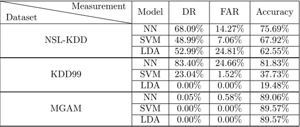
Table 5: Many-to-many. No time aspect. Reservoir size: 100. Connectivity: 20%.

Dataset Measurement Model DR FAR Accuracy

NSL-KDD SVMNN 68.09% 14.27%48.99% 7.06% 75.69%67.92% LDA 52.99% 24.81% 62.55% KDD99 SVMNN 83.40% 24.66%23.04% 1.52% 81.83%37.73% LDA 0.00% 0.00% 19.48% MGAM SVMNN 0.05%0.00% 0.58%0.00% 89.06%89.57% LDA 0.00% 0.00% 89.57%

8.2.

Many-to-one experiments

Finally, there are the ESNx, many-to-one, measurements. The attack/normal ratio of the KDD99 dataset still retained the same ratio as before even after being reduced by the reservoir, with both sequence lengths 10 and 20. This is due to the dataset containing mostly long sequences of either attacks or normal traffic. MGAM on the other hand increased to 66% attacks when being reduced with a sequence length of 10, and 88% attacks with sequence length 20. This happens because, for example, a sequence of 9 normal inputs and 1 attack will be reduced to a single vector that is classified as a sequence that contains an attack. A lot of normal traffic gets grouped with attacks. So only a sequence without any attacks is classified as normal. A reservoir size of 100 neurons was once again used, although this time with 5% connectivity.

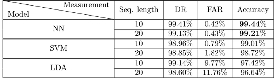
Table 6 show the results for the KDD99 dataset, with a sequence length of 10 and 20 inputs. The NN and SVM performed extremely well with both length 10 and 20, reaching a 99% accuracy with less than 1% false alarm rate. LDA didn’t perform quite as well due to a higher false alarm rate, but still 96% accuracy on length 20.

Table 6: KDD99. ESNx. Reservoir size: 100. Connectivity: 5%.

Model Measurement Seq. length DR FAR Accuracy

NN 10₂₀ 99.41%_99.13% 0.42%_0.43% 99.44_99.21%_% SVM 10₂₀ 98.96%_98.85% 0.79%_1.82% 99.01%_98.72% LDA 10₂₀ 99.14%_{98.60% 11.76%}9.77% 97.42%_96.64%

MGAM on the other hand, performed quite badly, as seen in Table 7. SVM classified almost everything as attacks and LDA did as well but not to the same degree as SVM. The NN instead classified very few as attacks, but those that it did classify as attacks it was generally correct on, as the false alarm rate is very low. The results of length 20 were terrible. Almost everything was classified as attacks, including from the NN this time.

Table 7: MGAM. ESNx. Reservoir size: 100. Connectivity: 5%.

Model Measurement Seq. length DR FAR Accuracy

NN 10₂₀ 13.29%_{91.00% 88.44%}0.48% 42.02%_82.34% SVM 10₂₀ 99.91%_{99.96% 100.00%}99.82% 66.34_88.90%_% LDA 10₂₀ 84.34%_98.25% 82.06%_97.65% 61.99%_87.64%

9.

Discussion

In this section, I will discuss the results and some reasons as to why experiments turned out as they did.

In several of the test cases, the models reached a point where they would classify a lot or almost everything as the same class in many-to-many mapping. Sometimes all as normal, sometimes all as attacks. I believe this is partially due to the time aspect of the reservoir taking over. The difference from normal to attack could have been toned down by the reservoir. A small difference that would normally indicate an attack might cause a similar change to something that is considered normal. Because of the tanh function the output values of the neurons were almost exclusively -1 or 1. Essentially making it a vector of binary values. A possible change would be to use another activation function that has a more gentle slope, to give more variation in the output values.

The MGAM dataset had the smallest percentage of attacks of the three datasets used, which may be a reason this happened. The attacks are also evenly spread out. If an attack were to occur every 10–20 steps then it either gets toned down or maybe the reservoir doesn’t have time to recover to a normal state. Although the latter is not very likely given that the NSL-KDD was classified decently and it had attacks occurring every couple steps throughout the whole series.

The LDA performed extremely well on MGAM without reservoir. It also performed decently on NSL-KDD and KDD99. But with the reservoir there was a significant decrease in accuracy. This is probably a side effect of the reservoir. LDA expects a gaussian distribution of the values of the features, and if it doesn’t get that then it won’t perform as well. The almost binary vector output from the reservoir probably did not work well with the LDA.

The high connectivity may also have affected this. A reservoir of size 100 with 20% connectivity was the values I found worked best overall when doing my experiments. Lower connectivity didn’t make the attacks stand out as much.

The experiments without the time aspect of ˙E ˙S ˙N showed that the time aspect didn’t have a huge impact, but it generally improved the neural network to have the time aspect. Otherwise, it didn’t have a huge impact in these cases. The classifiers still performed quite similarly with just having the input go through the random network. For some of the experiments, the reservoir was just overall not helpful. For this, it might’ve benefited to have a larger network and/or lower connectivity.

The accuracy of my experiments was not very good compared to the previous works of Alkas-assbeh et al. [1], Fu et al. [3], Shrivas and Dewangan [4]. The best I got with my reservoir was 77.51% on NSL-KDD and 85.09% on KDD99, both with the neural network. The reservoir did yield improvements most of the time for NN. SVM only improved on KDD99. While the accuracy increased on MGAM, it is not a valid measurement because it classified everything as normal. LDA on the other hand generally dropped a lot in accuracy with the reservoir. This means that it has some potential as a feature extraction method. What I believe would make a big difference is to before the reservoir use feature selection to get rid of features that are of little importance. Maybe even some other method of non-time-based feature extraction before applying the reservoir to get more value out of the reservoir. Any input features that are always the same or have nothing to do with attacks just create extra noise in the reservoir. With this, the connectivity in the reservoir could probably be reduced to be more sparse. Low sparsity (high density) means that changes will have a larger over-time effect on the reservoir. When attacks occur sparsely we don’t want the network itself to be too affected.

The many-to-one experiments with the ESNx reservoir worked relatively well. It classified the series of the KDD99 dataset very well as expected, with NN being the best and LDA worst. Although LDA still performed quite well. This is probably because the reservoir outputs had a larger difference in general here. KDD99 has long sequences of normal traffic and long sequences of attacks. So many times when there were attacks the whole series of length 10 or 20 would contain attacks. This made classification easier. The opposite was the case of MGAM. It contains few and sparse attacks so the sequences would instead look like normal traffic while containing a single attack that was toned down due to the other normal attacks in the sequence. A sequence of 9 normal and 1 attack will look very similar to a sequence of 10 normal inputs, especially if the attack is early in the sequence because the normal inputs will take over afterward. This made the models lean towards classifying everything as attacks because they couldn’t find much difference

between sequences of normal traffic and abnormal traffic. This is not unexpected. Classifying a sequence, of course, requires the input sequences to differ by some amount. If they are almost equal, as in the case of MGAM, it will be very hard to classify no matter what you do. Identifying if a sequence contains a single attack is probably easier to do by classifying the data separately. But if there are a lot of attacks at once then ESNx can perform well.

10.

Conclusion

In this thesis, I have attempted to use a reservoir network for feature extraction on both sequences as a whole (many-to-one mapping), and output on each timestep throughout a sequence to make use of the time aspect of reservoirs (many-to-many mapping). The purpose was to explore reservoir computing and compare different machine learning models for intrusion detection. I have measured the performance in terms of detection rate, false alarm rate, and accuracy. The many-to-many method was compared to the same learning models without the reservoir. The experiments used the datasets KDD99, NSL-KDD, and one unnamed which I chose to call MGAM in this thesis. They all contain labeled time series data of simulated network traffic with attacks.

The neural network paired quite well with the reservoir for many-to-many mapping. It showed improvements by using the reservoir versus not using it. LDA is not fit for this because with a reservoir the output format does not match what the LDA needs to create reliable predictions. None of my experiments got even close to that of previous works on IDSs. I used no form of feature selection/extraction beforehand for my experiments. I could likely improve the scores a lot by doing more preprocessing to only get relevant data into the reservoir, as unnecessary features will cause extra noise in the reservoir. Many-to-one (sequence feature extraction) was able to classify sequences very well when there was a clear difference, in the case of KDD99. On the MGAM dataset, it had awful performance because the attacks were sparse enough that the amount of normal traffic in a sequence took over the changes of a single attack. Reservoir computing could probably be used to identify DDoS attacks where there are massive waves of abnormal-looking requests in a real network. Although because it is based on a whole sequence it can’t predict completely in real-time as I used it. It will have to be adapted to fit such a use-case.

11.

Future Work

For future work, using feature selection before the reservoir can be done. I expect that it will increase accuracy as it will reduce the noise from unnecessary features in the reservoir. Changing the activation function of the reservoir or the neural network, or using completely different classifiers might also be worth exploring to achieve a better intrusion detection system.

References

[1] Mouhammd Alkasassbeh, Ghazi Al-Naymat, Ahmad Hassanat, and Mohammad Almseidin. Detecting distributed denial of service attacks using data mining techniques. International Journal of Advanced Computer Science and Applications, 7, 01 2016. doi: 10.14569/IJACSA. 2016.070159.

[2] Cynet. Network attacks and network security threats, 2020. URL https://www.cynet.com/ network-attacks/network-attacks-and-network-security-threats/. Last visited 2021-03-21.

[3] Y. Fu, F. Lou, F. Meng, Z. Tian, H. Zhang, and F. Jiang. An intelligent network attack detection method based on rnn. In 2018 IEEE Third International Conference on Data Science in Cyberspace (DSC), pages 483–489, 2018. doi: 10.1109/DSC.2018.00078.

[4] Akhilesh Kumar Shrivas and Amit Kumar Dewangan. Article: An ensemble model for classi-fication of attacks with feature selection based on kdd99 and nsl-kdd data set. International Journal of Computer Applications, 99(15):8–13, August 2014.

[5] Will Kenton. What is time series?, 2020. URL https://www.investopedia.com/terms/t/ timeseries.asp. Last visited 2021-03-21.

[6] Hung-Jen Liao, Chun-Hung Richard Lin, Ying-Chih Lin, and Kuang-Yuan Tung. Intrusion detection system: A comprehensive review. Journal of Network and Computer Applications, 36(1):16–24, 2013. ISSN 1084-8045. doi: https://doi.org/10.1016/j.jnca.2012.09.004. URL https://www.sciencedirect.com/science/article/pii/S1084804512001944.

[7] Peter Norvig and Stuart J Russel. Artificial Intelligence - A Modern Approach. Pearson Education Limited, 2010.

[8] Charu C Aggarwall. Data Classification Algorithms and Applications. Chapman & Hall/CRC, 2015.

[9] Jason Brownlee. Linear discriminant analysis for machine

learn-ing, April 2016. URL https://machinelearningmastery.com/

linear-discriminant-analysis-for-machine-learning/. Last visited 2021-05-04. [10] Mantas Lukoševičius and Herbert Jaeger. Reservoir computing approaches to recurrent neural

network training. Computer Science Review, 3(3):127–149, 2009. ISSN 1574-0137. doi: https: //doi.org/10.1016/j.cosrev.2009.03.005. URL https://www.sciencedirect.com/science/ article/pii/S1574013709000173.

[11] Justin Johnson. Lecture 10 | recurrent neural networks, 2017. URL https://www.youtube. com/watch?v=6niqTuYFZLQ. Stanford University, Last visited 2021-03-29.

[12] MathWorks. Feature extraction. URL https://se.mathworks.com/discovery/ feature-extraction.html. Last visited 2021-04-01.

[13] Witali Aswolinskiy, René Felix Reinhart, and Jochen Steil. Time series classifica-tion in reservoir- and model-space. Neural Process. Lett., 48(2):789–809, October 2018. ISSN 1370-4621. doi: 10.1007/s11063-017-9765-5. URL https://doi.org/10.1007/ s11063-017-9765-5.

[14] KDD, University of California, 1999. URL http://kdd.ics.uci.edu/databases/kddcup99/ kddcup99.html. Last visited 2021-05-04.

[15] Jason Brownlee. 3 ways to encode categorical variables for deep

learn-ing, November 2019. URL https://machinelearningmastery.com/

how-to-prepare-categorical-data-for-deep-learning-in-python/. Last visited 2021-05-05.