THE DETECTION OF A SN IIn IN OPTICAL FOLLOW-UP OBSERVATIONS OF ICECUBE NEUTRINO EVENTS
M. G. Aartsen1, K. Abraham2, M. Ackermann3, J. Adams4, J. A. Aguilar5, M. Ahlers6, M. Ahrens7, D. Altmann8, T. Anderson9, M. Archinger10, C. Arguelles6, T. C. Arlen9, J. Auffenberg11, X. Bai12, S. W. Barwick13, V. Baum10,
R. Bay14, J. J. Beatty15,16, J. Becker Tjus17, K.-H. Becker18, E. Beiser6, S. BenZvi6, P. Berghaus3, D. Berley19, E. Bernardini3, A. Bernhard2, D. Z. Besson20, G. Binder14,21, D. Bindig18, M. Bissok11, E. Blaufuss19, J. Blumenthal11,
D. J. Boersma22, C. Bohm7, M. Börner23, F. Bos17, D. Bose24, S. Böser10, O. Botner22, J. Braun6, L. Brayeur25, H.-P. Bretz3, A. M. Brown4, N. Buzinsky26, J. Casey27, M. Casier25, E. Cheung19, D. Chirkin6, A. Christov28, B. Christy19, K. Clark29, L. Classen8, S. Coenders2, D. F. Cowen9,30, A. H. Cruz Silva3, J. Daughhetee27, J. C. Davis15,
M. Day6, J. P. A. M. de André31, C. De Clercq25, H. Dembinski32, S. De Ridder33, P. Desiati6, K. D. de Vries25, G. de Wasseige25, M. de With34, T. DeYoung31, J. C. Díaz-Vélez6, J. P. Dumm7, M. Dunkman9, R. Eagan9, B. Eberhardt10,
T. Ehrhardt10, B. Eichmann17, S. Euler22, P. A. Evenson32, O. Fadiran6, S. Fahey6, A. R. Fazely35, A. Fedynitch17, J. Feintzeig6, J. Felde19, K. Filimonov14, C. Finley7, T. Fischer-Wasels18, S. Flis7, T. Fuchs23, M. Glagla11, T. K. Gaisser32, R. Gaior36, J. Gallagher37, L. Gerhardt14,21, K. Ghorbani6, D. Gier11, L. Gladstone6, T. Glüsenkamp3, A. Goldschmidt21, G. Golup25, J. G. Gonzalez32, D. Góra3, D. Grant26, P. Gretskov11, J. C. Groh9, A. Gross2, C. Ha14,21, C. Haack11, A. Haj Ismail33, A. Hallgren22, F. Halzen6, B. Hansmann11, K. Hanson6, D. Hebecker34, D. Heereman5, K. Helbing18, R. Hellauer19, D. Hellwig11, S. Hickford18, J. Hignight31, G. C. Hill1, K. D. Hoffman19, R. Hoffmann18, K. Holzapfe2, A. Homeier38, K. Hoshina6,39, F. Huang9, M. Huber2, W. Huelsnitz19, P. O. Hulth7, K. Hultqvist7, S. In24,
A. Ishihara36, E. Jacobi3, G. S. Japaridze40, K. Jero6, M. Jurkovic2, B. Kaminsky3, A. Kappes8, T. Karg3, A. Karle6, M. Kauer6,41, A. Keivani9, J. L. Kelley6, J. Kemp11, A. Kheirandish6, J. Kiryluk42, J. Kläs18, S. R. Klein14,21, G. Kohnen43,
R. Koirala32, H. Kolanoski34, R. Konietz11, A. Koob11, L. Köpke10, C. Kopper26, S. Kopper18, D. J. Koskinen44, M. Kowalski3,34, K. Krings2, G. Kroll10, M. Kroll17, J. Kunnen25, N. Kurahashi45, T. Kuwabara36, M. Labare33, J. L. Lanfranchi9, M. J. Larson44, M. Lesiak-Bzdak42, M. Leuermann11, J. Leuner11, J. Lünemann10, J. Madsen46, G. Maggi25, K. B. M. Mahn31, R. Maruyama41, K. Mase36, H. S. Matis21, R. Maunu19, F. McNally6, K. Meagher5, M. Medici44, A. Meli33, T. Menne23, G. Merino6, T. Meures5, S. Miarecki14,21, E. Middell3, E. Middlemas6, J. Miller25,
L. Mohrmann3, T. Montaruli28, R. Morse6, R. Nahnhauer3, U. Naumann18, H. Niederhausen42, S. C. Nowicki26, D. R. Nygren21, A. Obertacke18, A. Olivas19, A. Omairat18, A. O’Murchadha5, T. Palczewski47, H. Pandya32, L. Paul11,
J. A. Pepper47, C. Pérez de los Heros22, C. Pfendner15, D. Pieloth23, E. Pinat5, J. Posselt18, P. B. Price14, G. T. Przybylski21, J. Pütz11, M. Quinnan9, L. Rädel11, M. Rameez28, K. Rawlins48, P. Redl19, R. Reimann11, M. Relich36,
E. Resconi2, W. Rhode23, M. Richman45, S. Richter6, B. Riedel26, S. Robertson1, M. Rongen11, C. Rott24, T. Ruhe23, D. Ryckbosch33, S. M. Saba17, L. Sabbatini6, H.-G. Sander10, A. Sandrock23, J. Sandroos44, S. Sarkar44,49, K. Schatto10,
F. Scheriau23, M. Schimp11, T. Schmidt19, M. Schmitz23, S. Schoenen11, S. Schöneberg17, A. Schönwald3, A. Schukraft11, L. Schulte38, D. Seckel32, S. Seunarine46, R. Shanidze3, M. W. E. Smith9, D. Soldin18, G. M. Spiczak46,
C. Spiering3, M. Stahlberg11, M. Stamatikos15,50, T. Stanev32, N. A. Stanisha9, A. Stasik3, T. Stezelberger21, R. G. Stokstad21, A. Stössl3, E. A. Strahler25, R. Ström22, N. L. Strotjohann3, G. W. Sullivan19, M. Sutherland15, H. Taavola22, I. Taboada27, S. Ter-Antonyan35, A. Terliuk3, G. Tešić9, S. Tilav32, P. A. Toale47, M. N. Tobin6, D. Tosi6,
M. Tselengidou8, A. Turcati2, E. Unger22, M. Usner3, S. Vallecorsa28, N. van Eijndhoven25, J. Vandenbroucke6, J. van Santen6, S. Vanheule33, J. Veenkamp2, M. Vehring11, M. Voge38,63, M. Vraeghe33, C. Walck7, M. Wallraff11, N. Wandkowsky6, Ch. Weaver6, C. Wendt6, S. Westerhoff6, B. J. Whelan1, N. Whitehorn6, C. Wichary11, K. Wiebe10,
C. H. Wiebusch11, L. Wille6, D. R. Williams47, H. Wissing19, M. Wolf7, T. R. Wood26, K. Woschnagg14, D. L. Xu47, X. W. Xu35, Y. Xu42, J. P. Yanez3, G. Yodh13, S. Yoshida36, P. Zarzhitsky47, M. Zoll7
(IceCube Collaboration),
Eran O. Ofek51, Mansi M. Kasliwal52, Peter E. Nugent21,53, Iair Arcavi54,55, Joshua S. Bloom21,53, Shrinivas R. Kulkarni56, Daniel A. Perley56, Tom Barlow56, Assaf Horesh51,
Avishay Gal-Yam51, D. A. Howell54,57, Ben Dilday58 (for the PTF Collaboration),
Phil A. Evans59, Jamie A. Kennea30 (for the Swift Collaboration),
and
W. S. Burgett60, K. C. Chambers60, N. Kaiser60, C. Waters60, H. Flewelling60, J. L. Tonry60, A. Rest61, and S. J. Smartt62 (for the Pan-STARRS1 Science Consortium)
1
School of Chemistry & Physics, University of Adelaide, Adelaide SA, 5005 Australia
2
Technische Universität München, D-85748 Garching, Germany
3
DESY, D-15735 Zeuthen, Germany
4
Department of Physics and Astronomy, University of Canterbury, Private Bag 4800, Christchurch, New Zealand
5
Université Libre de Bruxelles, Science Faculty CP230, B-1050 Brussels, Belgium
6
Department of Physics and Wisconsin IceCube Particle Astrophysics Center, University of Wisconsin, Madison, WI 53706, USA
7
Oskar Klein Centre and Department of Physics, Stockholm University, SE-10691 Stockholm, Sweden
8Erlangen Centre for Astroparticle Physics, Friedrich-Alexander-Universität Erlangen-Nürnberg, D-91058 Erlangen, Germany 9
Department of Physics, Pennsylvania State University, University Park, PA 16802, USA
10
Institute of Physics, University of Mainz, Staudinger Weg 7, D-55099 Mainz, Germany
11
III. Physikalisches Institut, RWTH Aachen University, D-52056 Aachen, Germany
12
Physics Department, South Dakota School of Mines and Technology, Rapid City, SD 57701, USA
13
Department of Physics and Astronomy, University of California, Irvine, CA 92697, USA
14
Department of Physics, University of California, Berkeley, CA 94720, USA
15
Department of Physics and Center for Cosmology and Astro-Particle Physics, Ohio State University, Columbus, OH 43210, USA
16
Department of Astronomy, Ohio State University, Columbus, OH 43210, USA
17Fakultät für Physik & Astronomie, Ruhr-Universität Bochum, D-44780 Bochum, Germany 18
Department of Physics, University of Wuppertal, D-42119 Wuppertal, Germany
19
Department of Physics, University of Maryland, College Park, MD 20742, USA
20
Department of Physics and Astronomy, University of Kansas, Lawrence, KS 66045, USA
21
Lawrence Berkeley National Laboratory, Berkeley, CA 94720, USA
22
Department of Physics and Astronomy, Uppsala University, Box 516, SE-75120 Uppsala, Sweden
23
Department of Physics, TU Dortmund University, D-44221 Dortmund, Germany
24
Department of Physics, Sungkyunkwan University, Suwon 440-746, Korea
25
Vrije Universiteit Brussel, Dienst ELEM, B-1050 Brussels, Belgium
26
Department of Physics, University of Alberta, Edmonton, Alberta, T6G 2E1, Canada
27
School of Physics and Center for Relativistic Astrophysics, Georgia Institute of Technology, Atlanta, GA 30332, USA
28
Département de physique nucléaire et corpusculaire, Université de Genève, CH-1211 Genève, Switzerland
29
Department of Physics, University of Toronto, Toronto, Ontario, M5S 1A7, Canada
30
Department of Astronomy and Astrophysics, Pennsylvania State University, University Park, PA 16802, USA
31
Department of Physics and Astronomy, Michigan State University, East Lansing, MI 48824, USA
32
Bartol Research Institute and Department of Physics and Astronomy, University of Delaware, Newark, DE 19716, USA
33
Department of Physics and Astronomy, University of Gent, B-9000 Gent, Belgium
34
Institut für Physik, Humboldt-Universität zu Berlin, D-12489 Berlin, Germany
35
Department of Physics, Southern University, Baton Rouge, LA 70813, USA
36
Department of Physics, Chiba University, Chiba 263-8522, Japan
37
Department of Astronomy, University of Wisconsin, Madison, WI 53706, USA
38
Physikalisches Institut, Universität Bonn, Nussallee 12, D-53115 Bonn, Germany
39
Earthquake Research Institute, University of Tokyo, Bunkyo, Tokyo 113-0032, Japan
40
CTSPS, Clark-Atlanta University, Atlanta, GA 30314, USA
41
Department of Physics, Yale University, New Haven, CT 06520, USA
42
Department of Physics and Astronomy, Stony Brook University, Stony Brook, NY 11794-3800, USA
43
Université de Mons, 7000 Mons, Belgium
44
Niels Bohr Institute, University of Copenhagen, DK-2100 Copenhagen, Denmark
45
Department of Physics, Drexel University, 3141 Chestnut Street, Philadelphia, PA 19104, USA
46Department of Physics, University of Wisconsin, River Falls, WI 54022, USA 47
Department of Physics and Astronomy, University of Alabama, Tuscaloosa, AL 35487, USA
48
Department of Physics and Astronomy, University of Alaska Anchorage, 3211 Providence Dr., Anchorage, AK 99508, USA
49
Department of Physics, University of Oxford, 1 Keble Road, Oxford OX1 3NP, UK
50
NASA Goddard Space Flight Center, Greenbelt, MD 20771, USA
51
Department of Particle Physics and Astrophysics, The Weizmann Institute of Science, Rehovot 76100, Israel
52
The Observatories, Carnegie Institution for Science, 813 Santa Barbara Street, Pasadena, CA 91101, USA
53
Department of Astronomy, University of California, Berkeley, CA 94720, USA
54
Las Cumbres Observatory Global Telescope, 6740 Cortona Drive, Suite 102, Goleta, CA 93111, USA
55
Kavli Institute for Theoretical Physics, University of California, Santa Barbara, CA 93106, USA
56
Cahill Center for Astrophysics, California Institute of Technology, Pasadena, CA 91125, USA
57
Department of Physics, University of California, Santa Barbara, CA 93106, USA
58
North Idaho College, 1000 W Garden Ave, Coeur d’Alene, ID 83814, USA
59
Department of Physics and Astronomy, University of Leicester, Leicester, LE1 7RH, UK
60
Institute for Astronomy, University of Hawaii at Manoa, Honolulu, HI 96822, USA
61
Space Telescope Science Institute, 3700 San Martin Drive, Baltimore, MD 21218, USA
62Astrophysics Research Centre, School of Mathematics and Physics, Queenʼs University Belfast, Belfast, BT7 1NN, UK
Received 2015 June 9; accepted 2015 August 15; published 2015 September 18
ABSTRACT
The IceCube neutrino observatory pursues a follow-up program selecting interesting neutrino events in real-time and issuing alerts for electromagnetic follow-up observations. In 2012 March, the most significant neutrino alert during thefirst three years of operation was issued by IceCube. In the follow-up observations performed by the Palomar Transient Factory(PTF), a Type IIn supernova (SN IIn) PTF12csy was found 0°. 2 away from the neutrino alert direction, with an error radius of 0°. 54. It has a redshift of z= 0.0684, corresponding to a luminosity distance of about 300 Mpc and the Pan-STARRS1 survey shows that its explosion time was at least 158 days (in host galaxy rest frame) before the neutrino alert, so that a causal connection is unlikely. The a posteriori significance of the chance detection of both the neutrinos and the SN at any epoch is 2.2σ within IceCubeʼs 2011/12 data acquisition season. Also, a complementary neutrino analysis reveals no long-term signal over the course of one year. Therefore, we consider the SN detection coincidental and the neutrinos uncorrelated to the SN. However, the SN is unusual and interesting by itself: it is luminous and energetic, bearing strong resemblance to the SN IIn
63
2010jl, and shows signs of interaction of the SN ejecta with a dense circumstellar medium. High-energy neutrino emission is expected in models of diffusive shock acceleration, but at a low, non-detectable level for this specific SN. In this paper, we describe the SN PTF12csy and present both the neutrino and electromagnetic data, as well as their analysis.
Key words: circumstellar matter – galaxies: dwarf – neutrinos – shock waves – supernovae: individual(PTF12csy, SN 2010jl)
1. INTRODUCTION
IceCube is a cubic-kilometer-sized neutrino detector installed in the ice at the geographic South Pole between depths of 1450 and 2450 m(Achterberg et al.2006). It consists of an array of 5160 photon sensors, called Digital Optical Modules (DOMs), attached to 86 cables, called strings. Detector construction started in 2005 and finished in 2010 December. Neutrino observation relies on the optical detection of Cherenkov radiation emitted by secondary particles produced in neutrino interactions in ice or bedrock near IceCube. Due to the small neutrino interaction cross-section, the kilometer-scale detector has an effective area of only 0.25–10 m2 for muon neutrinos of 1–10 TeV energy (Aartsen et al.2014b). As part of the Optical Follow-up (OFU) program, the IceCube neutrino observatory records high-energy (HE) (∼100 GeV ...1 PeV) neutrino events at a rate of about 3 mHz, about 250 day−1. Those events are mostly( 90%~ ) cosmic-ray induced neutrinos from the atmosphere, referred to as atmo-spheric neutrinos, with about a 10% contamination of cosmic-ray induced atmospheric muons.
Routine neutrino analyses in IceCube, which are referred to as offline analyses, are performed after a certain amount of data, e.g., one or several years, has been collected. They benefit from events being put through computationally expensive reconstructions, as well as information on detector performance that become available only days or weeks after data acquisition. In contrast, neutrino analyses running online will not have access to such information, but have the advantage of being near real-time— results are available with a latency of∼3 minutes. With such a short latency neutrino analysis, multi-wavelength follow-up observations can be triggered by neutrino events. These follow-up data have the potential to reveal the electromagnetic counterpart of a transient neutrino source, which might otherwise be missed and thus be unavailable for further observations. In addition, the coincident detection of neutrino and electromag-netic emission can be statistically more significant and provide more information about the physics of the source than the neutrino detection alone. Another advantage of an online analysis is the prompt availability of the reconstructed neutrino dataset and thus the possibility of fast response analyses. Thus, IceCubeʼs online neutrino analysis efforts have also enabled fast γ-ray burst (GRB) searches like the one following GRB 130427A, published in a GCN Circular(Blaufuss2013).
The online search for short transient neutrino sources(on the order of 100 s) is mostly motivated by models of neutrinos from long duration GRBs (Waxman & Bahcall 1997; Becker et al.2006; Murase et al.2006; Murase2008) and from choked jet supernovae (SNe; Razzaque et al.2004; Ando & Beacom 2005). The two source classes are related: both are thought to host a jet, which is highly relativistic in case of long GRBs, but only mildly relativistic in case of choked jet SNe. Long GRB progenitors are conceived to be Wolf–Rayet stars that have lost their outer hydrogen and helium envelope (Meszaros 2006), while choked jet SNe can still have those outer layers(Ando &
Beacom2005), which are important for efficient HE neutrino production. The choked jet is more baryon-rich and has a much lower Lorentz factorG » than the GRB jet with3 G100. It cannot penetrate the stellar envelope and remains optically thick, making it invisible inγ rays. The neutrinos produced at TeV energies can escape nevertheless and may trigger the discovery of the SN in other channels. In particular, for a bright nearby SN, a neutrino detection would enable the acquisition of optical data during the rise of the light curve, strengthening the time correlation between the neutrino burst and the optical SN via the improved estimate of the explosion time (Cowen et al.2010). Mildly relativistic jets may occur in a much larger fraction of core-collapse SNe(CCSNe) than highly relativistic jets, i.e., GRBs(Razzaque et al.2004; Ando & Beacom2005). Detections of neutrinos from GRBs and choked jet SNe would be a remarkable discovery and could provide important insight into the SN-GRB connection and the underlying jet physics(Ando & Beacom2005). Both sources are expected to emit a short, about 10 s long burst of neutrinos (Ando & Beacom2005) either 10–100 s before or at the time of the GRB (if detectable) (Meszaros2006), setting the natural timescale of the neutrino search. After recording the neutrino burst, follow-up observations can be used to identify the counterpart of the transient neutrino source. A GRB can be identified either via the prompt γ-ray emission lasting up to about 150 s (Baret et al.2011) or via the optical and X-ray afterglow lasting up to several hours (Gehrels et al. 2004). The latter involves instruments of limitedfield of view and thus requires telescope slew, but has the advantage of much better angular resolution well below an arc minute(Gehrels et al.2004). A fast response within minutes to hours is required for a GRB afterglow follow-up. A choked jet SN is found by detecting a shock breakout or a SN light curve in the follow-up images, slowly rising and then declining within weeks after the neutrino burst. Following this scientific motivation, an online neutrino analysis, targeted at SN and GRB afterglow detection, was installed at IceCube in 2008(see Section2).
In addition to the transient neutrino emission within 100 s, as discussed above, SNe can be promising sources of HE neutrinos over longer timescales. In this paper, the class of SNe IIn(Schlegel1990; Filippenko1997) is explored further. These are CCSNe embedded in a dense circumstellar medium (CSM) that was ejected in a pre-explosion phase. Following the explosion, the SN ejecta plow through the dense CSM and collisionless shocks can form and accelerate particles, which may create HE neutrinos. This is comparable to a SN remnant, but on a much shorter timescale of 1–10 months (Murase et al.2011; Katz et al.2012).
SNe IIn(“n” for narrow) are spectrally characterized by the presence of strong emission lines, most notably Hα, that have a narrow component, together with blue continuum emission (Schlegel 1990; Filippenko1997). The narrow component is interpreted to originate from surrounding HIIregions, and the
high-density CSM(Schlegel1990). Since interaction of the SN ejecta with the dense CSM can lead to the conversion of a large fraction of the ejectaʼs kinetic energy to radiation, SNe IIn are on average more luminous than other SNe II (Richardson et al.2002). They generally fade quite slowly and some belong to the most luminous SNe (Filippenko 1997). There is much diversity within the subclass of SNe IIn (Filippenko 1997; Richardson et al. 2002), both spectroscopically and photome-trically, which can be explained by a diversity of progenitor stars and mass loss histories prior to explosion (Moriya & Tominaga 2012). Recently, there have been observations of eruptions prior to SN IIn explosions associated with mass loss which explain the existence of the dense CSM shells(e.g., Ofek et al.2014a).
In this paper, we report the discovery of a SN IIn in the optical observations triggered by an IceCube neutrino alert from 2012 March, and analyze the available neutrino and electromagnetic observations. The SN is already at a late stage at the time of the neutrino detection, which means that the neutrino-SN connec-tion is presumably coincidental. The paper is organized as follows. Section 2 introduces the OFU system of IceCube. Section 3 gives details about the neutrino alert triggering the follow-up observations that led to the SN discovery. Section 4 reports limits from a complementary offline neutrino search and X-ray limits. The UV and optical data that were obtained are discussed in depth in Section5. Wefinally summarize the results and give a conclusion in Section6.
2. THE OPTICAL AND X-RAY FOLLOW-UP SYSTEM In late 2008, an online neutrino event selection was set up at IceCube, looking for muons produced by charged current interactions of muon neutrinos in or near the IceCube detector. The analysis is running in real-time within the limited computing resources at the South Pole, capable of reconstruct-ing andfiltering the neutrinos and sending alerts to follow-up instruments with a latency of only a few minutes(Kowalski & Mohr2007; Abbasi et al.2012; Aartsen et al.2013).
The optical (OFU) and X-ray (XFU) real-time follow-up programs currently encompass three follow-up instruments: the Robotic Optical Transient Search Experiment (ROTSE; Akerlof et al. 2003), the Palomar Transient Factory (PTF; Law et al.2009; Rau et al.2009) and the Swift satellite (Gehrels et al. 2004). These triggered observations were supplemented with a retrospective search through the Pan-STARRS1 3π survey data (Kaiser 2004; Magnier et al. 2013), which is discussed further in Section5. In addition, there is also a real-time γ-ray follow-up program (GFU) targeting slower transients (timescale of weeks), e.g., flaring active galactic nuclei, that is sending alerts to the γ-ray telescopes MAGIC and VERITAS(Aartsen et al.2013).
The background of cosmic-ray induced muons from the atmosphere above the detector amounts to~106 muon events
per neutrino event. In afirst step, it is reduced by limiting the sample to the Northern Hemisphere, using the Earth as a muon shield and selecting only muon tracks that are reconstructed as up-going in the detector. Afterwards, cuts on quality parameters similar to those in Aartsen et al.(2014b) are applied to reject mis-reconstructed muon events: after an initial removal of likely noise signals, a chain of reconstructions is performed, which utilizes the spatial and temporal distribution of recorded photons on the DOMs. Starting with a simple linear track algorithm, more advanced reconstructions are employed, seeded with the
respective preceding reconstruction. The advanced reconstruc-tions maximize a likelihood that accounts for the optical properties of the ice for photon propagation (Ahrens et al. 2004). The final reconstruction in this chain is used to select events that are up-going in the detector. At this point, because of the vast amount of atmospheric muons, the data are still dominated by(down-going) muons that are mis-reconstructed as up-going. To reject this remaining background, high quality events are selected, where the selection parameters are derived from the value of the maximized track likelihood and from the number and geometry of recorded signals with a detection time compatible with unscattered photon propagation. Alternatively, events with a large number of total recorded photon signals are selected. The resulting analysis sample has an event rate of about 3 mHz, of which~90%are atmospheric muon neutrinos that have passed through the Earth and~10%are contamination of cosmic-ray induced muons from the atmosphere.
In the analysis sample, the median angular resolution of the neutrino direction is about 1° for a multi-TeV muon neutrino charged current interaction event, and 0°. 6 or less for 100 TeV and higher energies. The angular resolution of the sample is estimated using Monte Carlo(MC) simulation. Additionally, an estimator of the directional uncertainty is computed for each event, which is based on the shape of the reconstruction likelihood close to the found maximum(Neunhöffer2006). It is calibrated such that its median matches the MC derived angular resolution. We define the bulk of a sample as events within the central 90% of the energy distribution. The bulk of the main background contained in the analysis sample, atmospheric neutrinos, has energies between 160 GeV and 7 TeV. In contrast, the bulk of signal events from an unbroken En-2 power-law spectrum would have energies 1.2 TeV Eν 1.2 PeV. Signal neutrinos from GRBs are expected to follow a spectrum similar to En-2, which has cut-off energies between ∼1 PeV and ∼1 EeV (Murase & Nagataki 2006). Choked jet SNe are predicted to have lower cut-off energies around 20 TeV (Ando & Beacom2005) so that the overlap with atmospheric neutrinos is presumably much larger, while IIn neutrinos may have higher cut offs of 70–200 TeV (see Section4.1).
In order to suppress background from atmospheric neutrinos, a multiplet of at least two neutrinos within 100 s and angular separation of 3°. 5 or less is required to trigger an alert. In addition, since 2011 mid-September, a test statistic is used, providing a single parameter for selection of the most significant alerts. It was derived as the analytic maximization of a likelihood ratio following Braun et al. (2010), for the special case of a neutrino doublet with rich signal content:
T 2 ln 2 2 ln 1 exp 2 2 ln 100 s 1 q q A w 2 2 2 2 2
(
)
( ) ⎜ ⎟ ⎛ ⎝ ⎜⎜ ⎛⎝⎜ ⎞ ⎠ ⎟⎞ ⎠ ⎟⎟ ⎛⎝ ⎞⎠ l s ps q s =DY + - - - + Dwhere the time between the neutrinos in the doublet is denoted as D , and their angular separation as DY. The quantitiesT
q 2 1 2 2 2 s =s +s and w 1 1 2 1 2 2 2 1 ( ) s = s + s - depend on the
event-by-event directional uncertainties s and1 s of the two2
neutrino events, typically∼1°. The angleq corresponds to theA circularized angular radius of the field of view (FOV) of the follow-up telescope. It is set to 0°. 5 for Swift and 0°. 9 for ROTSE and PTF.
The test statistic λ is smaller for more signal-like alerts, which have small separation DY, small time differenceD andT a high chance to lie in the FOV of the telescope. Thus,λ is a useful parameter to separate signal and background alerts. For each follow-up program, a specific cut on λ is applied in order to send the most significant alerts to the follow-up instruments. In the 2011/12 data acquisition (DAQ) season, which is discussed here, a cut of l < -7.4 was used for the ROTSE follow-up, while cut values of−10.3 and −8.8 were used for PTF and Swift. Multiplets of multiplicity higher than two are passed directly to all follow-up instruments. Since the expected background rate is low(∼0.03 year−1), each observation of a triplet or higher order multiplet is significant by itself.
ROTSE (Akerlof et al. 2003) is a network of four optical telescopes with 0.45 m aperture and 1°. 85 × 1°. 85 FOV, located in Australia, Texas, Namibia and Turkey. Since late 2012, only the two Northern Hemisphere telescopes continue operation. ROTSE is a completely automatic and autonomous system that can receive alerts, perform observations and send resulting data without requiring human interaction. The limiting magnitude of ∼16–17 mag is however insufficient to discover faint or far SNe. For instance, for a very bright SN with−20 mag absolute magnitude, the detection radius is about 160–250 Mpc, while a faint SN with −17 mag is only visible within a radius of 40–65 Mpc. IceCube has been sending ∼25 alerts per year to ROTSE, since 2008 December. Thefirst 116 alerts, with a background expectation of 104.7 ± 10.2 alerts, were followed up with a median latency of 27.2 hr between the neutrino alert and start of the first follow-up observation.
PTF(Law et al.2009; Rau et al.2009) is a survey based at the Palomar Observatory in California, USA. It utilizes the 1.2 m Oschin Schmidt telescope on Mount Palomar. The focal plane is equipped with a mosaic of 11 CCDs with field of view of 7.26 deg2. The typical R-band limiting magnitude of PTF during dark time is about 21 mag. All the PTF data are reduced using the LBNL real-time pipeline responsible for transient identi fica-tion and the IPAC pipeline described in Laher et al.(2014). The image photometric calibration is described in Ofek et al.(2012). PTF pursues a number of science goals, most notably the discovery and observation of SNe. Several other telescopes in Palomar and at other locations can be used for photometric and spectroscopic follow-up observation. IceCube has been sending ∼7 alerts per year to PTF, since August 2010. The first 23 alerts, with a background expectation of 19.2 ± 4.4 alerts, were followed up with a median latency of 34.9 hr between the neutrino alert and start of thefirst follow-up observation.
Swift (Gehrels et al.2004) is a satellite operated by NASA and boards various instruments: a 170–600 nm ultraviolet/ optical telescope (UVOT), a 0.3–10 keV X-ray telescope (XRT) and a 15–150 keV hard X-ray Burst Alert Telescope (BAT). Swiftʼs main goal is the discovery and study of GRBs, of which it detects about 100 year−1(Lien et al.2014; one third
of all GRBs).64 IceCubeʼs X-ray follow-up program triggers Swiftʼs XRT, which can provide valuable information by observing a GRB afterglow in X-rays. The XRT has a FOV of only 0°. 4 in diameter, hence Swift performs seven pointings for each IceCube follow-up, resulting in an effective FOV of about 1° in diameter. IceCube has been sending ∼6 alerts per year to Swift, since 2011 February. The first 18 alerts, with a background expectation of 18.0 ± 4.2 alerts, were followed up with a median latency of 1.9 hr between the neutrino alert and start of the first follow-up observation (see Evans et al.2015).
3. NEUTRINO ALERT AND DISCOVERY OF PTF12CSY On 2012 March 30(MJD 56016), the most significant alert since initiation of the follow-up program (significance of
2.7s
~ , converting theλ cumulative distribution function value to single-sided Gaussian std. deviations) was recorded and sent to ROTSE and PTF simultaneously. The significance was also above the threshold for Swift(∼1σ), however it was within Swiftʼs moon proximity constraint,65 which delayed the observations by three weeks. The two neutrino events causing the alert happened on 2012 March 30 at 01:06:58 UT (MJD 56016.046505) and 1.79 s later, with an angular separation of 1°. 32. The combined average neutrino direction is at R.A. 6h57m45sand decl. 17°11′24″ in J2000 with an error radius of σw = 0°. 54. This average is a weighted arithmetic mean, weighting the individual directions with their inverse squared error, given by the event-by-event directional uncertainty(s.a.). The errors is dew fined after Equation (1). This assumes that the two neutrino events were emitted by a point source at a single fixed position. A variance of the individual true neutrino directions does not need to be taken into account, since the assumed intrinsic variance is zero in case of a point source. This leads to a relatively small error on the average direction. The main event properties are summarized in Table 1: the occurrence time on 2012 March 30, the reconstructed muon energy proxy Eˆm (see Aartsen et al. 2014), and the estimated directional error sY. The quantity Eˆm is a fit parameter and serves as a proxy for the muon energy, however it is not an estimator of the true muon energy. The energy En of the neutrino that produced the muon is not directly observable, since only the muon crossing the detector is accessible. However, using MC simulated neutrino events, one can use the muon energy proxy Eˆm to compare with MC events having a similar Eˆm value. From those MC events, a distribution of the true muon energy En can be derived, which depends on the assumed underlying neutrino energy spectrum. En probability density functions(PDFs) are filled with true energy values of
Table 1
Properties of the Neutrino Alert Events
Time(UT) sY(°) Eˆma(GeV) Enb(Atm.) (TeV) Enb(E-3) (TeV) Enb(E-2) (TeV)
01:06:58 0.96 1155 0.5-+0.42.9 0.7-+0.55.6 5.4-+5.0292.0
01:07:00 0.66 3345 0.9-+0.76.7 1.5-+1.314.8 15.7-+14.5611.5
Notes.
a
Eˆmis only a proxy correlated with muon energy, but not an estimator of the true muon energy.
b
Enis median neutrino energy with 90% C.L. error interval.
64
http://gcn.gsfc.nasa.gov/andhttp://grbweb.icecube.wisc.edu 65
MC events that have the reconstructed muon energy proxy Eˆm not more than 10% and the reconstructed zenith angle cos( )q not more than 0.1 away from the observed values of the two alert events. The median and the central 90% C.L. interval are calculated from the En probability density functions. The results are listed in Table 1, where the assumed neutrino spectrum is given in parentheses.
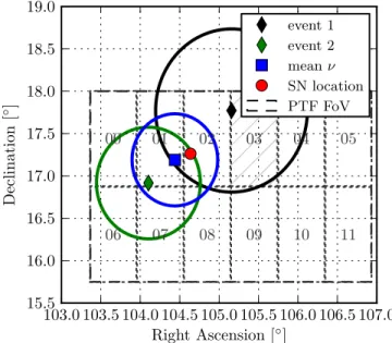
Follow-up observations at the direction of the neutrino alert were performed with multiple instruments(see Section5.1). In the PTF images, a CCSN, named PTF12csy, was discovered at R.A. 6h58m32s.744 and decl. 17°15′44″.37 (J2000), only 0°. 2 away from the average neutrino direction, see Figures1and2. This was a promising candidate for the source of the neutrinos, but a search of the Pan-STARRS1 archive (see Section 5.1) revealed that it was already at least 169 observer frame days old, i.e., 158 days in host galaxy rest frame, at the time of the neutrino alert. Therefore, it is highly unlikely that the neutrinos were produced by a jet at the SN site, as this is expected to happen immediately after core collapse in the choked jet scenario (Ando & Beacom2005).
However, steady neutrino emission on a timescale of several months is a possibility and explored in Section4.1.
3.1. Significance of Alert and SN Detection
The value of the test statistic λ for the neutrino doublet amounts to -18.1. The background distribution of λ is constructed from experimental data, containing mostly atmo-spheric neutrinos, by randomly permuting(shuffling) the event times and calculating equatorial coordinates, i.e., R.A. and decl., from local coordinates, i.e., zenith and azimuth angle, using the new times. That way, all detector effects are entirely preserved, e.g., the distribution of the azimuth angle, which has more events at angles where detector strings are aligned, and the time distribution, which is affected by seasonal variations. At the same time, all potential correlations between the events in time and space, and thus a potential signal, are destroyed.
The false alarm rate (FAR) for an alert withl-18.1is 0.226 year−1, calculated via integration of the λ distribution below−18.1. Considering the OFU live time of 220.1 days in the data acquisition season of the alert, 2011 September to 2012 May, yields N(l < -18.1)=0.136 false alerts. Hence, the probability, or p-value, for one or more alerts at least as
signal-like to happen by chance in this period is
P N
1 - Poisson(0; (l< -18.1))»12.7%. The OFU system had already been sending alerts to PTF for ∼460 days at the time of the alert. Scaling up the number of expected alerts with
18.1
l - , one derives a probability of ~24% during 460 days.
The estimated explosion time of SN PTF12csy does not fall within the a priori defined time window for a neutrino-SN coincidence of (1 day). It is thus not considered an a priori detection of the follow-up program. Despite this fact, for illustrative purposes, we calculate the a posteriori probability that a random CCSN of any type, at any stage after explosion, is found coincidentally within the error radius of this neutrino doublet and within the luminosity distance of PTF12csy, i.e., 300 Mpc. The number of such random SN detections is
N dN dt dV T m M r r dr 4 , , 4 2 s det 0 300 Mpc SN lim 2
(
ˆ)
( )ò
p p = Wwhere W is the solid angle of the doublet error circle (blues circle in Figure 1), which is ∼0.93 (°)2. For the volumetric CCSN rate dNSN (dt dV), a value of 0.78 × 10⁻⁴ Mpc−3year−1is used,(see Horiuchi et al.2013, Section 4.1). The control time T m( lim,M rˆ, ) is the average time window in which a SN is detectable, i.e., brighter than the limiting magnitude. It depends on the distance to the source r, the peak
Figure 1. Map of the sky with the two neutrino event directions, the average neutrino direction, and the location of SN PTF12csy. Estimated reconstruction errors are indicated with circles, the PTF FOV is shown as dashed box. The positions of the PTF survey camera CCD chips are plotted with dotted lines and the chip number is printed on each chipʼs field (cf. Law et al.2009). Note that
chip 03 is not operational and thus hatched in the plot.
Figure 2. New image, reference image and post-subtraction image of the PTF discovery of PTF12csy from 2012 April 09, with the location of PTF12csy in the center. This image shows only a small fraction of the PTF FOV. The image from the Sloan Digital Sky Survey (SDSS-III) DR12 (Gunn et al. 2006; Eisenstein et al. 2011; Ahn et al. 2014; Alam et al. 2015) is shown for
absolute magnitude Mˆ of the SN, the limiting magnitude mlim of the telescope, and the shape of the light curve which is adopted from a SN template web page by P. E. Nugent.66It is assumed that Mˆ follows a Gaussian distribution with mean −17.5 mag and standard deviation σ = 1 mag, based on Richardson et al.(2002). For PTF, mlim= (19.5 ± 1.0) mag is
assumed.
The resulting expectation value for coincidental SN detec-tions is Ndet»0.016, which results in a Poisson probability of
1.6%
~ to detect any CCSN within the neutrino alertʼs error radius. Combining this probability with the probability of 12.7% for the neutrino alert, Fisherʼs method (Fisher 1950, 1990; Littell & Folks1971; Brown1975) delivers a combined p-value of 1.4%, corresponding to a significance of 2.2σ. For the total live time of 460 days, the combined p-value is 2.5% which corresponds to a 2.0σ significance. This means, even ignoring the a posteriori nature of the p-value, a chance coincidence of the neutrino doublet and the SN detection cannot be ruled out and thus we consider the SN detection to be coincidental.
The following section reports about the available HE follow-up data. Limits on a possible long-term neutrino emission from PTF12csy are set using one year of IceCube data. Limits on the X-ray flux were obtained using the Swift satellite. Section 5 deals with the analysis of the low-energy optical and UV data as the SN detection is significant and interesting by itself.
4. HE FOLLOW-UP DATA 4.1. Offline Analysis of Neutrino Data
SNe IIn, such as PTF12csy, are a promising class of HE transients (see Murase et al.2011). The expected duration of neutrino emission from SNe IIn is 1–10 months, hence it is extremely unlikely that two neutrinos arrive within less than 2 s, so late after the SN explosion. However, to test the possibility of a long-term emission, a search for neutrinos from PTF12csy within a search window of roughly one year is conducted.
After the core-collapse of a SN IIn, the SN ejecta are crashing into massive CSM shells, producing a pair of shocks: a forward and a reverse shock. Cosmic rays (CRs) may be accelerated and multi-TeV neutrinos produced, potentially detectable with IceCube. The collisionless shocks generating the neutrinos are expected to generate X-rays as well at late times(see, e.g., Katz et al.2012; Svirski et al.2012; Ofek et al. 2013), but no X-rays were detected for PTF12csy, likely because of the large distance to the SN.
Following Murase et al.(2011) and Murase et al. (2014) (see also Katz et al. 2012), we model HE neutrino emission from PTF12csy. As a simplified approach, in order to get an order-of-magnitude estimate of the expected event rate, we perform the following calculation: the CSM density profile is calculated using(Murase et al.2014, Equations(4) and (A4)). The proton spectrum is modeled with a power law index- , as in (Murase2 et al.2014, Equation(A7)), with a cut-off energy given by the maximum energy of accelerated protons. The latter is determined by comparing the proton acceleration timescale either with the dynamical timescale (Murase et al. 2014, Equation (28)), or, if pp energy losses are relevant, with the cooling timescale (Murase et al. 2014, Equation (30)). The
lower of the two maximum energies is the one that needs to be considered. The proton spectrum is normalized to the total CR energy ECRby assuming that a fraction of the kinetic energy of
the ejecta Eej is converted into CRs, that is ECR=CREej
(compare Murase et al.2014, Equations(3), (25), using CSM shell mass MCSM SN ejecta mass Mej). Other model
parameters are the break-out radius Rbo and shock velocity
vshock. The expected neutrino spectrum from pp interaction is
derived from the semi-analytical description in Kelner et al. (2006), taking into account the meson production efficiency (Murase et al.2014, Equations(35), (36)). It is distance-scaled and folded with IceCubeʼs effective area from Aartsen et al. (2014b) to obtain the expected number of events. It is found that inserting commonly assumed values (Murase et al.2011, 2014; Margutti et al.2014) of Eej=10Ebol=2.1 ´ 1051erg (with the bolometric energy found in Section5.2.5),CR=0.1, Mej= 10 M☉, Rbo» 6 × 1015cm, and vshock» 5000 km s−1, on
average only 0.07 IceCube neutrino detections are expected. Despite the low expectation for the neutrino fluence, we search for a long-term neutrino signal from PTF12csy in the IceCube data. As a more elaborate approach compared to the simplified approximation described above, we test the neutrino emission models A and B given in Figure 1 of Murase et al. (2011), which are two representative cases of CR accelerating scenarios: model A corresponds to a CSM shell with a high density of 1× 1011cm−3at a small radius of 1 × 1015.5cm, while model B is the opposite with a density of 1× 107.5cm−3 at radius 1 × 1016.5cm. For the ejecta, a kinetic energy of 1 × 1051erg, a velocity of 1 × 10⁴km s−1, and a mass of several solar masses, lower than the CSM mass, are assumed. Model A is close to a scenario explaining superluminous SNe IIn such as SN 2006gy, while model B is a good description for dimmer, but longer lasting SNe like SN 2008iy. Both models have a neutrino energy spectrum close to E-2,
with a cut-off energy around 70 TeV for model A, around 84 TeV for the forward shock (FS) in model B, and around 275 TeV for the reverse shock (RS) in model B. In model A, only the reverse shock is of importance for CR acceleration. The suggested emission timescales are 1 × 10⁷s = 115 days for model A and 1× 107.8s= 366 days for model B (Murase et al.2011).
Figure 3 shows the model fluences scaled down to a luminosity distance of 308 Mpc. We analyze about one year of IceCube data: the entire IceCube 86 strings data acquisition season 2011/12, from 2011 May 13 to 2012 May 15. The long search window is motivated by the large uncertainty on the explosion date (between 2011 March 21 and October 13) as well as the long duration of neutrino emission for some scenarios like∼700 days for model B in Murase et al. (2011). For simplicity, we assume that the entire fluence was emitted during the 1 year search window. We use the neutrino sample of the IceCube optical follow-up system and perform a statistical point source analysis of neutrino events close to the position of the SN, based on Braun et al.(2008).
Each neutrino candidate event i is given both a signal and background probability Si and Bi which are combined in the likelihood function n n NS n N B 1 . 3 s i N s i s i 1 ( ) ⎜⎛ ⎟ ( ) ⎝ ⎞ ⎠ =
+ -=The variable nsis the number of signal events contained in the sample, which isfitted to maximize the likelihood, and N is the 66
total number of selected neutrino candidate events. The signal probability Si is the product of the spatial Gaussian PDF and the energy PDF P E( i∣ )f , i.e. the probability of a signal event having reconstructed energy Eigiven the neutrino spectrumf of the source(derived from Monte Carlo simulation):
x x x x S , , ,E 1 P E 2 exp 2 . 4 i i i s i i i s i i 2 2 2
(
)
(
)
( ) ⎛ ⎝ ⎜⎜ ⎞⎠⎟⎟ s ps s f = --Here,s is the eventʼs angular error estimate, xi i is the eventʼs reconstructed direction, and xs the SN or neutrino source position. The background probability Bi contains the energy PDF and a normalization constant for the background from atmospheric neutrinos.
We define the test statistic as likelihood ratio (Braun et al.2008) n 2 log 0 , 5 s
( )
( ) ˆ ( ) ⎡ ⎣ ⎢ ⎢ ⎤ ⎦ ⎥ ⎥ l =-serving as a powerful test for separating the null hypothesis from the hypothesis of signal event contribution. Here, nˆ is thes number of signal events that maximizes the likelihood and corresponds to the most likely description of the data.
The result of the maximum likelihoodfit is nˆs=0 both for models A and B, i.e., we see no sign of signal contribution in our neutrino event sample. We set 90% C.L. Neyman upper limits (see Neyman1937, reprinted in Neyman 1967) on the tested neutrino fluence models, which amount to ∼1500 and ∼1300 times the fluences given for models A and B above, respectively. The limits are much higher than the fluence prediction because of IceCube being insensitive to SNe IIn at such large distances. Figure 3 shows a plot of the tested neutrinofluence and the limits set using 1 year of IceCube data. This null result and the large distance to the SN further support our conclusion that the SN detection was coincidental. Nevertheless, it is interesting to roughly estimate the hypothetical emitted neutrino fluence: we take the median neutrino energies of the two alert neutrinos from Table 1 and
look up the effective areas for the OFU neutrino sample at the respective energies. From this, we derive a hypothetical neutrinofluence of 3.2 × 10⁻⁴erg cm−2for a source spectrum
E 2
µ - (E
ν = 5.4, 15.7 TeV), or 10.8 × 10⁻⁴erg cm−2 for a source spectrumµE-3(E
ν= 0.7, 1.5 TeV). Assuming that this neutrino fluence was emitted by the SN, this would imply a radiated neutrino energy of∼3.4 × 1051erg or∼1.2 × 1052erg using the luminosity distance of∼300 Mpc, corresponding to about 15 or about 50 times the radiated electromagnetic energy of Ebol= 2.1 × 1050erg(see Section5.2.5). This is higher than
what can be expected, since with reasonable assumptions that the explosion energy Eej10Ebol (Margutti et al. 2014;
Murase et al.2014) and a fractionCR0.1of it going into CRs(Murase et al.2011), the energy in neutrinos should be on the same order or less than Ebol. Thus, also with a simple energetic argument, isotropic neutrino emission from PTF12csy causing the neutrino alert is implausible, especially on a timescale of seconds. However, a beamed emission from a jet with a small opening angle of<30° would in principle be possible.
4.2. X-Ray Observations of PTF12csy
The Swift satellite observed the SN four times, on 2012 April 20(MJD 56037) and around 2012 November 15 (MJD 56246) (see Table2). We perform source detection using the software developed for the 1SXPS catalog(Evans et al.2014) on each of the four observations, and on a summed image made by combining all the datasets. No counterpart to PTF12csy is detected. Upper limits are generated for each of these images, following Evans et al.(2014). A 28″ radius circle centered on the optical position of PTF12csy is used to measure the detected X-ray counts c at this location, and the expected number of background counts cbg, predicted by the background
map created in the source detection process. We then use the Bayesian method of Kraft et al.(1991) to calculate the 3σ upper limit cULon the X-ray count rate of PTF12csy, using the XRT
exposure map to correct for anyflux losses due to bad pixels on the XRT detector, and thefinite size of the circular region.
The upper limit count rate is converted to unabsorbedfluxFUL
using the HEASARC Tool WebPIMMS,67assuming a blackbody model with T= 0.6 keV as in Miller et al. (2010b), a Galactic hydrogen column density of 1.31× 1021cm−2(Willingale et al. 2013)68and a redshift of z=0.0684. The result is a 0.2–10 keV X-rayflux < 4.6 × 10⁻¹⁴erg cm−2s−1 for the most constraining
Figure 3. Neutrino fluence at Earth from PTF12csy (solid lines) and derived upper limits set by IceCube (dashed lines, corresponding gray scales) as function of energy for the tested models A, B reverse shock (RS), and B forward shock(FS) from Murase et al. (2011).
Table 2
Swift XRT observations of PTF12csy
Time(MJD) Exposure(ks) c cbg cUL FUL 56037.15 4.9 1 1.47 1.3 4.6 56245.29 2.0 1 0.62 2.1 7.4 56246.04 1.2 2 0.44 9.8 30.0 56247.62 5.0 2 1.35 2.1 7.4 Sum 13.0 6 3.71 1.3 4.6
Note. Energy range: 0.2–10 keV. c: measured counts within a 28″ aperture. cbg:
expected background counts within the same aperture. cUL: 3σ upper limit on
the X-ray count rate in 10−3s−1.F : upper limit on the unabsorbed source fluxUL
in 10−14erg cm−2s−1.
67https://heasarc.gsfc.nasa.gov/Tools/w3pimms.html 68
upper limits, corresponding to a 0.2–10 keV X-ray luminosity of LX< 5.2 × 1041erg s−1 with a luminosity distance of about 308 Mpc. Using a power-lawµE-2instead of a blackbody as
an alternative X-ray emission model, the unabsorbedflux upper limit becomes <7.4 × 10⁻¹⁴erg cm−2s−1, and hence, LX < 8.4× 1041erg s−1.
Comparing with other SNe IIn, e.g., SN 2008iy(Miller et al. 2010b) which had a measured X-ray luminosity of LX= (2.4 ± 0.8) × 1041erg s−1 or SN 2010jl (Ofek et al. 2014b) with LX ≈ 1.5 × 1041erg s−1, we cannot exclude X-ray emission from PTF12csy with our measured upper limit. However, Svirski et al. (2012) suggest that LX be about 10-4 of the bolometric luminosity at the time of the shock breakout. With the estimated bolometric luminosity from Section5.2.5around the time of the first Swift observations, this implies LX ≈ 6.4× 1038erg s−1, well below our X-ray limits.
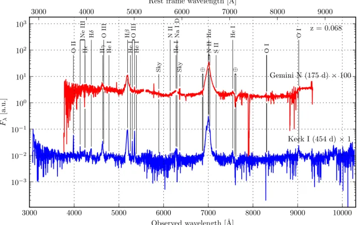
5. LOW-ENERGY FOLLOW-UP DATA 5.1. Optical and UV Observations of PTF12csy During the follow-up program of the neutrino alert, thefirst observations were done on 2012 April 03, 05, 07 and 09(MJD 56020 to 56026) by PTF with the Palomar Samuel Oschin 48-inch telescope (P48; Law et al. 2009), which is a wide-field Schmidt telescope. The images(see Figure2) revealed a so far undiscovered SN, named PTF12csy, at a magnitude of∼18.6 in the Mould R-band. More photometric observations were carried out, with the P48 and the Palomar 60-inch (P60) telescopes (Law et al. 2009) at the Palomar Observatory in California, and the Faulkes Telescope North (FTN) (Brown et al. 2013) at Haleakala on Maui, Hawaii. Spectroscopy was taken as well, with the Gemini North Multi-Object Spectrograph (GMOS; Hook et al. 2004) on the 8 m Gemini North telescope (Mauna Kea, Hawaii) on 2012 April 17 (MJD 56034) and with the Low-resolution Imaging Spectrometer (LRIS) (Oke et al. 1995) on the 10 m Keck I telescope (Kamuela, Hawaii) on 2013 February 09 (MJD 56332), enabling the identification of the SN as a SN IIn with narrow emission lines. The spectra are available from WISeREP69 (Yaron & Gal-Yam2012).
P48 data were extracted using an aperture photometry pipeline and are calibrated with 21 close-by SDSS stars(Gunn et al. 2006; Eisenstein et al. 2011; Ahn et al. 2014; Alam et al.2015). The faint host galaxy was subtracted and the upper limits are at the 5σ level. P48 magnitudes are in the PTF natural AB magnitude system, which is similar, but not identical to the SDSS system. The difference is given by a color term, which is ignored in this work, except for the conversion of Mould R to SDSS r, explained in Section 5.2.1. The P60 photometry is tied to the same 21 SDSS calibration stars. Note that there might be host galaxy contamination in the late-epoch P60 photometry. P60 magnitudes are in the SDSS AB magnitude system. The FTN data were processed by an automatic pipeline, without host subtraction, and agree very well with the host-subtracted P60 data taken in the same night. The Pan-STARRS1(PS1) telescope was not part of the real-time triggering and response system, but its wide-field coverage provides a useful archive to search retrospectively for detections. PS1 is a 1.8 m telescope located at Haleakala on Maui in the Hawaiian islands, equipped with a 3°. 3 FOV and a
1.4 gigapixel camera (Kaiser 2004). In the course of its 3π steradian survey, the telescope observes each part of the sky typically 8–10 times per year (Magnier et al.2013). PS1 first detected PTF12csy on MJD 55847.582 and archived it as object PSO J104.6365+17.2622. The magnitudes in all PS1 images were obtained with PSFfitting within the Pan-STARRS Image Processing Pipeline(Magnier2006). They are calibrated to typically seven local SDSS DR8field stars. The magnitudes are in the natural PS1 AB system as defined in Tonry et al. (2012), which is similar, but not exactly the same as SDSS AB magnitudes. Particularly the g-band can differ.
The Swift UVOT data were analyzed using the publicly available Swift analysis tools(Nasa High Energy Astrophysics Science Archive Research Center (Heasarc), 2014),70 and a source was seen close to the detection threshold.
ROTSEʼs limiting magnitude of about 16–17 mag prevented a detection of the SN in ROTSE follow-up observations.
5.2. Photometry
5.2.1. Photometric Corrections
The photometry is corrected for Galactic extinction using RV =AV E B( -V)=3.1and E B( -V)=0.071(Schlegel et al. 1998).71 The extinction coefficient is converted to the filters’ effective wavelengths using the algorithm from Cardelli et al.(1989),72i.e., 0.35 mag for u, 0.30 mag for B, 0.26 mag for g, 0.19 mag for r, 0.11 mag for z. The extinction within the host galaxy could not be determined.
In Figure4, the Gemini North spectrum is overlaid with the applied photometricfilters. The strong Balmer lines contribute differently to the various filters. For the spectral energy distribution(SED) construction (see Section5.2.5), in order to approximate the blackbody continuum, the contribution of the strongest emission lines, Hα and Hβ, is removed from the photometry using the Gemini North spectrum and the filter
Figure 4. Background, gray, left axis: Gemini North spectrum from 2012 April 17(MJD 56034). Foreground, multiple colors, right axis: the filter response functions of the applied photometricfilters, defined as filter transmission or effective area. Note that the absolute normalization is arbitrary and only the shape of the curves is relevant.
69
http://wiserep.weizmann.ac.il
70
Seehttp://www.swift.ac.uk/analysis/uvot/for instructions
71
Obtained via the NASA/IPAC Infrared Science Archive http://irsa. ipac.caltech.edu/applications/DUST/
72
curves. For Figures6and 7, the P48 Mould R magnitudes are converted to SDSS r by subtracting the Hα contribution (as above), applying the formulae in Ofek et al. (2012) valid for blackbody spectra, and then re-adding the Hα contribution to the r-band. After conversion, the P48 R magnitudes are consistent with the P60 SDSS r magnitudes.
The Swift UVOT data contain host contamination. Since no GALEX data from a pre- or post-SN epoch are available for the host galaxy,73no host subtraction can be done in the UVfilters of UVOT. For the u, b and vfilters, the host is subtracted by interpolating the host magnitudes from the SDSS DR12 data (Alam et al.2015)74to the effective wavelengths of the UVOT filters.
5.2.2. The Light Curves
The earliest detection of PTF12csy was in the Pan-STARRS1 y-band on 2011 October 13 (MJD 55847.582), 169 days prior to the neutrino alert in observer frame, corresponding to 158 days in host galaxy rest frame using z= 0.0684 (see Section5.3). The latest non-detection, again in Pan-STARRS1, was on 2011 March 21 (MJD 55641.3) in a 30 s z-band frame, 206 days before thefirst detection (193 days in rest frame). Hence, the explosion time is not well constrained and can be anytime between MJD 55641.3 and MJD 55847.6. Hereafter, we refer to the y-band detection at MJD 55847.582 as the first detection and use it as day 0 for the light curve.
The uncorrected SN light curves with the data available through the IceCube OFU program are displayed in Figure 5, including photometry acquired with the Swift UVOT filters uvw2, uvm2, uvw1, u and b; the Johnson B filter on P60; the SDSS filters g, r, i with data from P60, PS1, and FTN; the SDSS zfilter on P60; Mould R filter on P48; and Pan-STARRS yfilter on PS1. The entire uncorrected photometry in apparent magnitudes, as seen in Figure 5, is also available in Table3.
The light curves are averaged within bins of 10 days width, for each filter and telescope separately. Note that, in contrast to most of the other photometry, no host subtraction is performed for the Swift UVOT magnitudes presented in Figure 5 and Table3.
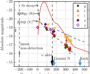
Figure6shows the light curve of selectedfilters in absolute magnitudes, after the photometric corrections. Light curves of other exceptional SNe II are overlaid for comparison: SN IIn 2006gy (Ofek et al. 2007; Smith et al. 2007; Kawabata et al.2009; Miller et al.2010a), one of the most luminous SNe ever recorded, and SN 2010jl (Stoll et al. 2011; Zhang et al. 2012), a SN IIn that is spectroscopically similar to PTF12csy(see Section5.3) and shows signs of a collisionless shock in an optically thick CSM, hinting toward potential HE neutrino production(Ofek et al.2013). Note that the SN 2010jl light curve is not extinction corrected and the comparison light curves have different reference dates: SN 2010jl is relative to maximum light, 2006gy is relative to the explosion time. A theoretical light curve from pure radioactive decay of
Ni Co Fe
56 56 56 (black dashed line) is added to the figure
as well, scaled to match the observed absolute magnitude of PTF12csy.
The brightest observed absolute magnitudes after application of photometric corrections(see Section5.2.1) and converting to absolute magnitudes with a distance modulus ofm = 37.443 (z=0.0684) are Mg ≈ −19.0 mag, Mr ≈ −19.0 mag, Mi ≈ −19.6 mag, Mz≈ −19.4 mag, and My≈ −19.0 mag, assuming standard cosmology with Hubble parameter H0 = 70 km s−1 Mpc−1, matter density W =m 0.3, and dark energy density
0.7
W =L . While these are lower limits to the peak magnitude due to the sparse sampling, these absolute magnitudes are relatively modest compared to the most luminous SNe IIn, e.g., SN 2006gy (MR = −22 mag) (Kawabata et al. 2009) or SN 2008fz (MV= −22.3 mag) (Drake et al. 2010). They are however comparable to the SNe IIn 2008iy(Mr≈ −19.1 mag) (Miller et al. 2010b), 1988Z (MR −18.9 mag) (Turatto et al. 1993) and SN 2010jl (MR −20.0 mag) (Zhang et al.2012).
5.2.3. Decline Rates and Energy Source
The light curves of PTF12csy indicate a plateau within ∼100 days after first detection, and a slow fading afterwards. The corrected absolute magnitude light curves are fitted to obtain the linear decline rates in different photometric filters, during different epochs(see Figure7 and Table 4). For some epochs andfilters, especially g and r, the decline rates are close to 0.98 mag (100 days)−1, the decline rate expected for radioactive 56Co decay(Miller et al. 2010b), while in general decline rates are slower, indicating that at least part of the radiated energy is powered by interaction of the SN ejecta with a dense CSM(Miller et al.2010b).
Additionally, radioactive decay of 56Co at a still relatively high absolute magnitude of ∼−19 mag implies a preceding 56
Ni decay with an extremely bright peak, which was not observed, although the data are quite sparse. Assuming that the luminosity is generated by radioactive decay alone and following Kulkarni (2005), we estimate that 1.7 M☉ of56Ni
would be required to provide the bolometric luminosity of 9.7× 1042erg s−1at 100 days in rest frame(see Section5.2.5). The lower limit on the 56Ni mass is set by assuming that the explosion and thus generation of56Ni was at the latest possible time, directly before the first detection. Figure 6 shows the
Figure 5. PTF12csy photometry in apparent magnitudes without applying corrections. The photometry is averaged over intervals of 10 days. The data originate from the following telescopes: uvw2, uvm2, uvw1, u, b: UVOT; B: P60; g: P60, PS1, FTN; r: P60, PS1, FTN; R: P48; i: P60, PS1, FTN; z: P60, PS1; y: PS1. 73 Seehttp://galex.stsci.edu/GalexView/ 74 http://skyserver.sdss.org/dr12/en/tools/chart/navi.aspx
Table 3
Photometric Observations of PTF12csy
MJD Date Rest Frame Days Mag Abs. Mag Lim. Mag Filter Tel.
55273.219 −537.589 L L 21.11 g P48 55294.162 −517.987 L L 20.62 R P48 55431.514 −389.429 L L 18.99 R P48 55477.402 −346.478 L L 20.67 R P48 55596.889 −234.642 L L 18.90 g P48 55641.304 −193.071 L L 21.40 z PS1 55847.588 0.005 18.52± 0.08 −18.92 L y PS1 55875.515 26.145 18.00± 0.02 −19.45 L i PS1 55937.502 84.163 18.17± 0.04 −19.27 L z PS1 55948.816 94.752 18.82± 0.05 −18.62 L g PS1 55948.841 94.776 18.66± 0.02 −18.79 L r PS1 55957.475 102.858 19.00± 0.02 −18.44 L g PS1 55967.269 112.024 18.23± 0.01 −19.22 L i PS1 55997.366 140.194 18.80± 0.08 −18.64 L y PS1 56022.981 164.169 18.61± 0.08 −18.84 18.23 R P48 56026.246 167.225 19.01± 0.08 −18.43 L z PS1 56034.841 175.270 19.47± 0.04 −17.98 L r P60 56034.844 175.273 18.99± 0.08 −18.46 L z P60 56035.177 175.584 18.64± 0.04 −18.80 L R P48 56035.922 176.281 18.68± 0.03 −18.76 L i P60 56035.925 176.284 20.15± 0.06 −17.30 L B P60 56035.928 176.287 19.69± 0.05 −17.75 L g P60 56036.581 176.899 18.66± 0.04 −18.78 20.97 i FTN 56036.585 176.902 19.54± 0.06 −17.90 21.12 r FTN 56036.590 176.906 19.73± 0.07 −17.72 21.23 g FTN 56037.150 177.431 L L 19.13 v UVOT 56037.150 177.431 20.60± 0.35 −16.84 20.79 u UVOT 56037.150 177.431 22.21± 0.28 −15.23 22.76 uvm2 UVOT 56037.150 177.431 22.52± 0.36 −14.92 22.71 uvw2 UVOT 56037.150 177.431 L L 21.84 uvw1 UVOT 56037.150 177.431 19.46± 0.27 −17.98 19.95 b UVOT 56039.175 179.326 18.74± 0.03 −18.70 L i P60 56039.177 179.328 19.55± 0.04 −17.89 L r P60 56039.178 179.329 20.17± 0.06 −17.28 L B P60 56039.181 179.332 19.73± 0.04 −17.71 L g P60 56040.285 180.365 18.60± 0.07 −18.85 20.98 i FTN 56043.178 183.073 18.70± 0.05 −18.74 L R P48 56158.504 291.015 19.40± 0.12 −18.05 L i P60 56161.496 293.815 20.58± 0.12 −16.86 L r P60 56163.490 295.682 19.69± 0.13 −17.76 L i P60 56165.486 297.550 21.01± 0.15 −16.44 L g P60 56176.465 307.826 20.73± 0.26 −16.72 L g P60 56177.453 308.751 20.07± 0.26 −17.37 L r P60 56185.431 316.218 19.72± 0.11 −17.73 L i P60 56185.432 316.219 20.77± 0.17 −16.68 L r P60 56185.436 316.223 20.92± 0.15 −16.53 L g P60 56200.887 330.685 19.81± 0.30 −17.63 L i P60 56202.385 332.086 21.09± 0.25 −16.35 L r P60 56215.381 344.250 21.23± 0.39 −16.21 L r P60 56215.429 344.295 20.11± 0.10 −17.33 L i P60 56215.435 344.301 21.25± 0.17 −16.19 L g P60 56219.344 347.960 21.16± 0.13 −16.28 L g P60 56219.837 348.421 20.97± 0.13 −16.47 L r P60 56224.988 353.242 20.01± 0.17 −17.44 L i P60 56229.808 357.754 20.20± 0.45 −17.24 L i P60 56246.320 373.208 22.71± 0.26 −14.73 23.34 uvw2 UVOT 56246.320 373.208 22.55± 0.35 −14.89 22.79 uvw1 UVOT 56246.320 373.208 L L 23.05 uvm2 UVOT
corresponding theoretical light curve resulting from the radio-active decay of nickel and cobalt(black dashed line). Adopting an earlier explosion time results in an even larger 56Ni mass.
This is much more than the usual amount of56Ni of<0.5 M☉,
often <0.1 M☉(see, e.g., Pejcha & Thompson 2015, also
Margutti et al. 2014). However, extremely superluminous SNe might have56Ni masses of that order of magnitude (Gal-Yam2012).
We note that in addition to the 56Ni mass and luminosity arguments, the spectrum showing intermediate width Balmer lines and a continuum appears inconsistent with radioactive decay as well (see Section5.3).
5.2.4. Fitting to an Interaction Model
Here we assume that the light curve is powered by conversion of the ejectaʼs kinetic energy to luminosity through interaction of the ejecta with the CSM. Following Ofek et al.(2014b; see also: e.g., Chugai & Danziger1994; Svirski et al.2012; Moriya et al.2013), we model the light curve as a power law of the form L t( ) =L t0 a.
After shock breakout, there is a phase of power-law decline of the luminosity, with an index of typicallya » -0.3. This lasts until the shock runs over a CSM mass equivalent to the ejecta mass and the shock enters a new phase of either conservation of energy if the density is low enough and the gas cannot cool quickly(the Sedov–Taylor phase), or conservation of momentum if the gas radiates its energy via fast cooling(the snow-plow phase). During the late stage, the light curve will be declining more steeply, in both cases(Ofek et al.2014b).
Since we assume PTF12csy to be powered by interaction, we try tofit the interaction model from Ofek et al. (2014b) to the light curve data with the least-squares method. We perform the fit within the range of 93–200 rest frame days, starting at the first r-band detection, and use the r-band light curve scaled with the bolometric luminosity from Section5.2.5. It is found that the power-law index α needs to be significantly steeper than−0.3 in order to reasonably describe the data. It lies in the range of−3 to −1.2, using the constraint on the explosion time (see Section 5.2.2) for the temporal zero point of the power-law. The best fit is at a = - , with the explosion3 time at the lowest allowed value which is the date of the last non-detection. This suggests a very steep CSM density profile
r 5
µ - (see Ofek et al.2014b, Equation (12)), compared to the
profile rµ -2 resulting from a wind with steady mass loss.
However, the self-similar solutions of the hydrodynamical equations(Chevalier1982) that are used in (Ofek et al.2014b, Equation(12)) are invalid if the CSM density profile is steeper than r-3. But nevertheless, as discussed for the late-time light
curve in(Ofek et al.2014b, Section 5.2), probably the profile is steeper than r-3.
This leaves us with several possible explanations.
1. Already between rest frame days 93 and 200, the SN was in the late, e.g., snow-plow, phase. This is consistent with SN 2010jl, where the late-time light curve also shows a power-law index a » - (Ofek et al.3 2014b, Section 5.2). Assuming that the break in the light curve between power-law phase and late phase occurred just before the first r-band detection at day 93, and comparing with SN 2010jl(Ofek et al. 2014b), then this means that the SN was likely already a few hundred days old, and the
Figure 6. PTF12csy photometry (symbols) in absolute magnitudes, with correction for Galactic extinction, and conversion of P48 Mould R magnitudes to SDSS r magnitudes (see Section 5.2.1). The data originate from the
following telescopes: g: P48, P60, PS1, FTN; r: P48, P60, PS1, FTN; i: P60, PS1, FTN; z: P60, PS1; y: PS1. The photometry is averaged over intervals of 10 days. Other absolute SN II light curves(lines) and a theoretical light curve from radioactive decay of nickel(black dashed line) are added for comparison. The comparison light curves are partly not extinction corrected and have different reference dates(see the text).
Figure 7. Light curves of several filters with the fitted linear declines. See Table4for the numerical values of the found decline rates.
Table 4
Decline Rates of the PTF12csy Light Curve
Filter 0–150 daysa 70–200 daysa 170–400 daysa
uvw2 L L 0.097± 0.227 g L 1.127± 0.044 0.893± 0.051 r L 0.974± 0.053 0.907± 0.059 i 0.269± 0.024 0.656± 0.089 0.764± 0.052 z 0.943± 0.079 L y 0.199± 0.080 L L Note.
aUnits: mag(100 days)−1. Indicated periods in rest frame days relative tofirst
r-band maximum was about 1–1.25 mag brighter than the observed one(see Ofek et al.2014b, Figure 1), consistent with SN 2010jlʼs r-band maximum. It follows that the power-law phase ended 286 rest frame days after explosion, from which we can derive a swept CSM mass of12 M☉, using Ofek et al.(2014b, Equation(22)) and
adopting the standard values given for SN 2010jl. 2. The SN is powered by ejecta-CSM interaction, but its
light curve is declining steeper than a t-0.3 power law.
This is possible, e.g., if spherical symmetry, assumed in Ofek et al.(2014b), is broken, if the optical depth is lower than in SN 2010jl or if the CSM density profile falls steeper than r-2(s.a.).
3. The SN is not powered by interaction, but by radioactive decay, leading to an exponential light curve decline. However, this appears unlikely, as noted above in Section 5.2.3.
5.2.5. Spectral Energy Distribution(SED)
Since the spectra are only roughly calibrated, the SED is approximated from photometric data. For the highest spectral range and number of observations, a window of 10 observer frame days around day 189, from day 184 to 194, is used to select data(day 172.2 to day 181.6 in rest frame). Photometric corrections are applied, e.g., Hα and Hβ removed (see Section 5.2.1). The data are plotted in Figure8 as function of the filters’ effective wavelengths. A blackbody spectrum is assumed to describe the SED and isfitted to the data. For each filter, a model data point corresponding to the blackbody spectrum is calculated via integration of the blackbody spectrum and thefilter function following the SDSS definition of AB magnitude in(Fukugita et al.1996, Equation(7)). Ac2
fit minimizes the difference between the model data and the measured data.
The fit results in a reduced 2 n 7.9 5 1.6
dof
c = = and
delivers estimates for both the rest frame temperature T and the absolute bolometric luminosity Lbolof the photosphere emitting
the blackbody radiation: T= (7160 ± 270) K and Lbol= (5.53 ± 1.18) × 1042
erg s−1, where the errors correspond to 1σ. Applying the Stefan–Boltzmann law, we can calculate the radius of the blackbody photosphere from the bolometric luminosity. We estimate it to be Rphot= (1.7 ± 0.1) × 1015cm. Finally, to obtain an estimate on the total radiated energy, the lines’ contributions to the luminosity have to be added to the continuum luminosity. Using the Gemini North spectrum, the contribution of the Hα and Hβ line to the total luminosity is computed and added to the continuum luminosity from the blackbody fit. This results in an estimated total radiated luminosity of (6.4 ± 1.2) × 1042erg s−1 at day 189 in the observer frame, i.e., day 177 in the rest frame.
We use the fitted shape of the i-band light curve (see Section5.2, Figure7, Table4) to extrapolate this value and find a total radiated luminosity of∼9.7 × 1042erg s−1 at 100 days (rest frame), as used in Section5.2.3, and a total energy of Ebol
= 2.1 × 1050
erg radiated within 400 rest frame days afterfirst detection, comparable to SN 2008iy which had∼2 × 1050erg (Miller et al.2010b) and SN 2010jl with 4.3 × 1050erg(Zhang et al.2012). This is a lower limit on the total radiated energy, since we lack photometric data between explosion and first detection and do not extrapolate before the first detection. Additionally, as discussed below, we are neglecting a possible contribution of X-ray andγ-ray emission to the total radiated energy, which is not considered by the blackbody spectrum based on the UV and optical data.
We recommend to treat these results with caution, since Ofek et al.(2014b) pointed out that at late times the fraction of energy released from SNe IIn in X-rays can increase, causing the optical spectrum to deviate from a blackbody as fewer photons are available in the optical. This can lead to an effective decrease of the estimated photospheric radius. In this context, our estimates of Rphot, Lbol, and Ebolmust be treated as lower limits. Unfortunately, the X-rayflux from PTF12csy was not detected(see Section4.2).
5.3. Spectroscopy
Two spectra were acquired (Table 5, Figure 9). They are dominated by narrow emission lines, characteristic for SNe IIn, with a very weak blue continuum, which indicates the old age of the SN. No continuum is visible in the late spectrum. The SN emission lines are primarily hydrogen, the Balmer series is visible from Hα up to Hò. The oxygen lines OI ll7772, 7774, 7775, 8447, OII l3727 with FWHM
≈500 km s−1, and OIII ll4364, 4960, 5008 with FWHM ≈ 350 km s−1are very narrow and were most likely produced by circumstellar gas released by the progenitor prior to explosion and then photoionized by UV radiation(Filippenko1997).
Figure 10 shows a close-up on the Hα line from both spectra, plotted versus Doppler velocity relative to the rest
Figure 8. SED of PTF12csy using photometry from 10 days around day 189 (observer frame) after the first detection. The fitted rest frame temperature is T = (7160 ± 270) K and the fitted bolometric luminosity (5.53 ± 1.18) × 1042erg s−1.
Table 5
Log of Spectral Observations MJD Tdisc Tdet D (km sv
−1) Instrument
56034 11 175 80 Gemini North GMOS
56332 290 454 100 Keck I LRIS
Note. Tdisc: rest frame days after PTF discovery. Tdet: rest frame days afterfirst
detection by PS1.D : spectral resolution at the Hα line at 7014 Å in observerv