2-D model study of the influence of the surface on mesoscale convection during the Indian monsoon, A

DURING THE INDIAN MONSOON

by

Roger A.

Pielke, P.I.

NSF Grant # ATM-8915265

Department of Atmospheric Science

Colorado State University

Zejin Xian

Department of Atmospheric Science Colorado State University

Fort Collins, Colorado Summer, 1991

A 2-D MODEL STUDY OF THE INFLUENCE OF THE SURFACE ON MESOSCALE CONVECTION DURING THE INDIAN MONSOON

A two-dimensional Colorado State University Regional Atmospheric Modeling System model is used to simulate a summer monsoon cloud cluster and its associated mesoscale convective system observed over the Bay of Bengal on 3-8 July 1979. Summer Monsoon Experiment (SMONEX) data is applied to initialize the model. A modification of the Kuo convective parameterization and microphysical process are employed in the simulations.

The simulated monsoon cloud cluster forms over the ocean and propagates westward to the land with the upper tropospheric easterly flow. Mesoscale convection appears over the land when the monsoon cloud cluster approaches the coast. The landfalling cloud cluster brings ralnfall inland. The maximum 24 hour precipitation appears in the region of 200-300 km west of the coastline.

Sensitivity simulations are performed for a variety of land characteristics and water surface temperatures. The major conclusions of these tests are:

1. Wetter soil is more conducive for the formation of mesoscale convective systems because it supplies more moist static energy to them. Therefore, more precipitation is intercepted on the wetter ground surface.

2. Rough land promotes more mesoscale convection and produces stronger upward motion in the landfalling cloud cluster than smooth land. However, the simulated precipitation does not have an apparent increase when the land roughness is enlarged.

later. The rainfall is concentrated in a narrow range between 100 to 300 km west of the coast.

iii

Zejin Xian

Department of Atmospheric Science Colorado State University

Fort Collins, Colorado 80523 Summer, 1991

I would first like to thank my advisor, Dr. Roger A. Pielke, for his support and guidance during this study. His helpful suggestions and ideas on many of the modelled mesoscale convection related aspects of this work are greatly appreciated. I would also like to thank my other committee members, Dr. Robert L. Grossman, Dr. Richard H. Johnson, and Dr. Paul W. Mielke for useful discussions and comments which improved the text. Dr. Grossman's thorough review of my study and Professor Johnson's suggestions on summer monsoon research are especially appreciated.

Drs. Craig Tremback and Bob Walko are thanked for answering many model-related questions. Dr. Mel Nicholls provided initial help in modelling cloud problems. Mr. Xubin Zeng and Dr. Mike Weissbluth are thanked for several helpful discussions concerning this work.

This study was supported by the National Science Foundation (NSF) under Grant #ATM-8915265. The computing was done on the CRAY X-MP and Y-MP at the National Center for Atmospheric Research (NCAR) and the Stardent super workstation at the Department of Atmospheric Science, Colorado State University.

Dallas McDonald in acknowledged for her professional preparation of the paper.

2.2 Numerical Methods . . . . 10

2.3 Physical Parameterizations 10

3 The Model Simulations 12

3.1 Observations and Model Initializations 12

3.2 Development Stage . 23

3.3 Decayed Stage . . . 44

4 Sensitivity Experiments 54

4.1 Soil Moisture Sensitivity. . . 55

4.2 The Influence of Surface Roughness 62

4.3 Sea Surface Temperature Variation 77

4.4 Low SST and Dry Land Surface 94

5 Summary and Conclusions 100

5.1 Summary of the Modeling Results . 100

5.2 Conclusions... . 101

REFERENCES 104

APPENDIX 111

1.1 The low-level flow of summer monsoon. 1.2 Tropic cloud structure. . . .

3.1 Satellite picture of the Indian summer monsoon at (a) OOz, 7 July 1979; and

2

6

(b) OOz 8 July 1979. . . . 14

3.2 Observation outline of cloud shield. . . 15 3.3 Echo pattern of depression. . . 16

3.4 24 hour observed rajnfaJI at OOZ, 8 July 1979. 17

3.5 (a) Initial sounding ofthermal structure.. . . 19

3.5 (b) East-west wind component. . . 20 3.6 (a) Two hour model simulation of vertical velocity w with cold low-level and

warm high-level initial perturbation. . . .. 21 3.6 (b) Twelve hour model simulation of vertical velocity w with cold low-level and

warm high-level initial perturbation. . . 22

3.7 (a) Convective heating rate of the control run at 0500 LST. 24 3.7 (b) Vertical velocity w ofthe control run at 0600 LST. . . 25 3.8 (a) Control run at 1000 LST for vertical velocity w. . . . 27 3.8 (b) Control run at 1000 LST for virtual potential temperature perturbation (/I~). 28 3.8 (c) Control run at 1000 LST for total ice mixing ratio. . . .. 29 3.9 Variation of averaged sensible and latent heat flux over land and ocean of the

control run agajnst time. . . 30 3.10 (a) Control run at 1300 LST for convective heating rate. . 32 3.10 (b) Control run at 1300 LST for vertical velocity w. . . . 33 3.11 (a) Control run at 1400 LST for vertical velocity w. . . . 34 3.11 (b) Control run at 1400 LST for convective heating rate. . 35 3.11 (c) Control run at 1400 LST for total ice mixing ratio. . . 36 3.12 The variation of the soil moisture with time of the control run at 100 west of

the coastline. . . 37 3.13 (a) Vertical velocity w of the control run at 1600 LST. . 39 3.13 (b) West-east wind u of the control run at 1600 LST. 40 3.14 Precipitation of the control run at 1700 LST. . . 41 3.15 Rajn mixing ratio of the control run at 1700 LST. . . . 42 3.16 Variation of low-level west-east wind u of the control run 50 km west of the

coast agajnst time. . . .. 43 3.17 (a) Virtual potential temperature perturbation (/I~) at 2000 LST of the control

run. . . . 45 3.17 (b) Rajn mixing ratio at 2000 LST of the control run. . . 46 3.17 (c) Equivalent potential temperature at 2000 LST of the control run. . 47 3.18 Vertical velocity w of the control run at 2200 LST. . . 48

4.5 Variation of low level west-east wind u of SRS (rough soil surface) and SMS

(smooth soil surface) ... _ . . . 67

4.6 (a) Convective heating rate at 1200 LST for SRS run. . . . 69

4.6 (b) Convective heating rate at 1200 LST for SMS run. . . .. 70

4.7 The lower level (0-4500 m) east-west wind of the SRS and SMS run at 1400 LST. 71 4.8 Variation of averaged land surface latent heat flux of SRS and SMS case with time. . . 72

4.9 (a) Variation of soil moisture of SRS and SMS run with time. . . 73

4.9 (b) Variation of surface temperature of SRS and SMS run with time. . . . 74

4.10 (a) W field at 1600 LST of SRS run. . . 75

4.10 (b) W field at 1600 LST of SMS run.. . . 76

4.11 (a) Convective heating rate at 1600 LST of SRS run. . . 78

4.11 (b) Convective heating rate at 1600 LST of SMS run. . . . 79

4.12 Total precipitation of control, SRS, and SMS run at 2200 LST. . . 80

4.13 (a) Convective heating rate at 1200 LST of SHT (higher sea surface tempera-ture) simulation. . . . . . . 82

4.13 (b) Convective heating rate at 1200 LST of SLT (low sea surface temperature) simulation. . . . 83

4.14 (a) W field at 1400 LST for SHT run . . . 85

4.14 (b) W field at 1400 LST for SLT run. . . . 86

4.15 (a) W field at 1600 LST for SHT run. . . 87

4.15 (b) W field at 1600 LST for SLT run. . . . 88

4.16 Total precipitation of SHT and SLT run at 2200 LST. . . 89

4.17 (a) W field at 2200 LST for SHT run . . . 90

4.17 (b) W field at 2200 LST for SLT run. . . . 91

4.18 Eighteen hour simulated precipitation of SHT and SLT run at 0200 LST. 93 4.19 (a) Convective heating rate of SLM run at 1400 LST. . . . . 95

4.19 (b) Ice mixing ratio of SLM run at 1400 LST. . . .. 96

4.20 W field of SML (dry soil and low sea surface temperature) simulation at 1500 LST. . . .. 98 4.21 Distribution of the precipitation of 14, 16, and 18 hour simulation of SLM run. 99

3.1 Basic Parameters Used in the Simulations.. . . .. 12

the Arabian Sea, (2) deep convection and heavy rainfall along the southern edge of the Tibetan Plateau, (3) terrain convection associated with the Western Ghats, (4) Bay of Bengal depressions, and (5) mid-tropospheric cyclones over the northeastern Arabian Sea and northern Bay of Bengal.

Figure 1.1 gives the low-level circulation and significant convection features in the summer monsoon regions. Throughout the monsoon period, a variety of very significant cyclonic disturbances develop over the Bay of Bengal. The statistics (ICSU /WMO, 1976) show that about two monsoon depressions per month form over the Bay of Bengal, and move westward or northwestward inland and bring large amounts of precipitation over the eastern Indian continent.

In 1979, the Summer Monsoon Experiment (SMONEX) was carried out in the Bay of Bengal (ICSU /WMO, 1976; Fein and Kiettner, 1980). This experiment was designed to study the southwesterly monsoon

in

the vicinity of the Indian subcontinent. It

is

known that the typical scale of depressions in this region is around 500 km in the formative stage. Although the depressions form in the northern part of the Bay of Bengal, they do not reach hurricane intensity because they stay over the ocean only a short time period and the large vertical wind shear over the troposphere inhibits a local accumulation of the latent heat released in the disturbance.

Figure 1.1: The low level flow of summer monsoon (adopted from Johnson and Houze, 1987).

depression reached 1.5 x 10-4 _{s-l around the center. The zonal mean wind was westerly}

above 600 hPa. There existed large northward momentum :fluxes around 600 hPa. The analysis of divergence indicated that the maximum convergence appeared around 700 hPa on July 7 with a value of -3 x 10-5 _{s-l. Upper-level divergence existed around 200 hPa}

and was near 2 x 10-5 _s-l.

Sanders (1984) found that the ra.in from the Bay of Bengal depression was generated in numerous convection towers. The ra.in was distributed with the storm-scale ascent area and had a mesoscale precipitation feature.

Houze and Churchill (1987) analyzed the mesoscale precipitation features associated with the Bay of Bengal depression. They found that the precipitation occurred in a mesoscale ra.in area of 100-300 km in the horizontal dimension and each of them conta.ined intense convective cells. Each mesoscale precipitation feature was characterized by a widespread cloud shield base at about the 400 hPa level. The ra.in falling from the cloud deck was partly convective and partly stratiform. Some of the convective towers were very intense and overshot the top of the cloud shield. The convective region consisted of an arc-shaped, southward moving line of intense convective ra.in oriented generally east-west and followed to the north by a wide region of stratiform clouds and precipitation. The orientation and structure of the arc lines may relate to the strong easterly monsoonal shear in this region. The large mesoscale precipitation features tended to be elongated from the west-east to the northwest-southeast.

On the coast, substantial precipitation occurred after 0300 GMT on the 6th and ended by 0300 GMT on the 8th as the depression center passed inland (Sanders, 1984). Mter the system moved into the Indian peninsula, a substantial vertical separation was

produced as the 850 hPa center moved northwestward and the 500 hPa center westward with a speed of 5 m S-1.

1.2 The Structure of the Monsoon Depression Over the Bay of Bengal

The structure of the Bay of Bengal depression based on observations has been in-vestigated by many researchers, e.g., Koteswaram and George (1958), Krishnamurti et al. (1975), and others. Their studies are mainly concerned with the structure of the depression as it moved inland over central India.

A typical depression had a warm core in the lower troposphere during its develop-ing stage over the ocean. After it fully developed, the depression developed a cold core structure in the lower troposphere and a warm core in the upper troposphere (Krishna-murti, 1975; Godbole, 1977). The warm area in the depression was also an area with a relative humidity higher than 90%. Therefore, a large mass of clouds associated with the depression formed when the depression moved westward toward the Indian coast.

Warner (1984) summarized the core structure of the depression on 7 July 1979 as sloped toward the southwest with height, with buoyant cloudy ascent within the cold air to the south and west of the axis, and warm subsidence of clear air to the northwest of the axis. The convergence near the cloud base reached values of nearly -2 x 10-4 _{s-1 in areas}

of ~300 km2 to the south and west of the center with divergence and subsidence of a similar magnltude to the northeast of the center. Warner and Grumm (1984) further found that the area covered by the updrafts was 0.5% in cumulus. The cloudy ascent was sustained upward through the 700 hPa level only in a mesoscale line of cumulus clouds. This line lasted 3 hours and propagated faster than the low-level wind. Mid-level stratus (700-200 hPa) and cumulus dominated the total cloud coverage. The cloud mapping showed that the cumulus generally penetrated to above 9 km. A dense high overcast based around 7.5

km had embedded cumulus. However, the total cloud was dominated by mid-level thin fragmentary stratus and cumulus debris. Warner and Grumm further confirmed that the ascent in the lower troposphere was concentrated in mesoscale features of cumulus clouds covering nearly 1% of the inner area of the depression.

the summer. The latent heat released by the cumulus convection yields an increase of the temperature within the clouds. These increased temperatures then drive a stable ascent of the saturated air to produce stable latent heating where there is a cold air core and low air pressure.

Sanders (1984) found that the thermal stratification near the depression over the Bay of Bengal above 850 hPa is approximately moist-adiabatic. The wind analyses showed that the basic zonal currents, westerly in the lower troposphere and easterly in the middle levels, were weakened as the depression formed. The convective heating released from a number of convective towers and the large scale wind shear were the major mechanisms supporting the depression. Houze (1989) suggested a typical cloud system structure as in Fig. 1.2. He emphasized the microphysical and kinematic aspects of the precipitation processes in the convection and stratiform regions.

1.4 Landscape Effects on the Local Convection

There are a number of research works that study the effects of mountains (Grossman and Durran, 1984) and offshore flow forced by the terrain (Dudhia, 1989) on monsoon con-vection. However, there is little work concerning the influence of landscape characteristics on monsoon convection.

Physick (1980) showed the relative contributions of sensible and latent heat fluxes on the inland penetration rate of sea breezes. Large values of sensible heat provided more direct heating to the atmosphere, thereby resulting in a large horizontal pressure gradient and more rapid inland propagation of the sea breeze. The characteristics of landscape, as verified by many researchers in recent years (e.g., McCumber and Pielke, 1981; Garrett,

CONVECTIVE

f /

SHOWERS '--.j/ • SmA TIFORM' REGION /

,I

"""' ... "-00,,""""" -

-

--

.J--

40' C -Mean~t/ (l0'5anIS~ HEAVIER STRATIFORM RAIN I RADAR BRIGHT BAND ldean Desamt ('Usanls)

Figure 1.2: Tropic cloud structure (from Houze, 1989).

1982; Anthes, 1984; PieIke, 1984; Segal et al., 1984; Pielke and Segal, 1986; MaMou! et al.,

1987: etc.) are importa.nt in in1Iuencing the development of the mesoscale system over la.nd through the in1Iuence on the magnitUde of surface latent a.nd sensible heat fluxes to the atmosphere. These fluxes (i) directly in1Iuence energy available for cumulus convection, a.nd (li) can create mesoscale circulation as strong as a sea breeze (e.g., Segal et aI., 1988) when a spatial gra.dient in la.ndscape type results in large horizontal gra.dients of sensible heat fluxes.

Generally, on a wet la.nd surface, the increased latent heat fluxes through soil mois-ture flux a.nd evaporation of intercepted rain will increase the moisture supply to the atmosphere (Ookouchi et aI., 1984). Mahfouf et aI. (1987) a.nd La.nicci et aI. (1987) sum-marized that the low soil moisture over the Mexica.n plateau allowed the development of a deep mixed layer, thereby increasing severe storm activity in that area. Ya.n a.nd Anthes (1988) compared the sea breeze circulation over dry a.nd moist la.nd. For a relative dry surface, they found that the upward motion associated with the sea breeze front generated

precipitation than that of the dry land sea breeze.

The landfall decay process of tropical cyclones and its associated rainfall distribution can be significantly influenced by land surface conditions (Tuleya et al., 1984). Pie1ke and Zeng (1989) suggested that severe thunderstorms were more likely over irrigated areas than over adjacent dry prairie land since the added water vapor provided greater buoyant energy for the cumulus cloud convection.

Nicholls et al. (1990) found that formation of deep convection associated with the sea breeze over the Florida peninsula was related to soil moisture content. The dry soil simulation generated rapidly developing sea-breezes which moved inland quickly, whereas the wet soil run produced a much more slowly developing sea breeze.

In the Bay of Bengal and Indian coast region, warm and moist tropical air is significant in the evolution ofthe monsoon depression. Based on observations, Keshavamurty (1971) suggested that the significant association between vorticity at 900 hPa and observed rain-fall distribution indicated the important role of Ekman pumping and CISK (conditional instability of the second kind) mechanisms to explain the future growth of the depression over the Indian continent. Webster (1983,1987) suggested that surface hydrological effects can influence the 10 to 20 days variation of the Indian su=er monsoon.

1.5 Working Hypothesis of the Study

Based on the previous discussions, the following hypothesis is made. The monsoon depression forms over the Bay of Bengal where the cumulus anvil shears to the west by the strong easterly flow above 400 hPa. The high-level anvil moves inland ahead of the landfalling depression and brings rainfall and reduces the incoming solar radiation

reaching the ground. Therefore the normal sea breeze (Lohar and Chakravarty, 1990) does not occur due to the decrease of the temperature gradient between the land and the sea. The anvil rainfall increases the soil moisture well to the west of the surface depression and makes the environment for the next cluster more conducive to deep convection, since a substantial latent heat source would be present over the land in the form of warm, wet soil. The warm, wet soil would subsequently modify the boundary layer air over it producing higher moisture static energy. Given a favorable mid- and upper tropospheric wind and thermodynamic environment, the next cluster would propagate further inland before weakening occurs. This study will test this hypothesis by using a numerical model to identify relationships between land surface characteristics and inland characteristics of Bay of Bengal mesoscale convective systems which have moved from ocean to land.

Based on the previous discussions, it seems that in order to represent the mesoscale convective system during the summer monsoon season properly, a numerical model for this purpose needs the following characteristics. First, the model should have a realistic convective cloud parameterization to represent mesoscale cloud development associated with convective transport of heat and moisture. Second, there should be a microphysical parameterization that can reproduce the observed ice-dominated stratiform anvil clouds and their associated latent heating. Third, a radiation transfer parameterization should be included in the model to represent the impact of anvil clouds on the infrared and solar radiation heating process as on land. Finally, a realistic soil-atmosphere parameteriza-tion is needed to represent the momentum and heat flux transfer from the Earth to the atmosphere. A detailed description of the model is given in Chapter Two.

8v 8v 8v

8

II 8v

8

Z 8v

8t

=

-u 8x - w 8z - fu

+

8x (Km 8x)+ 8z (Km 8z) (2.2) Thermodynamic equation

88;1

= _

88;1 _ 88;1

+

!...(Kh 88;1) !...(KZ 88;r) (88;1)

+(

88;1) (88;1) (2 3) 8t u 8x w 8z 8x h 8x

+

8z II 8z

+

8t CO" 8t r ••

+

8t rad •

Moisture and condensation mixing ratio continuity equations (n = 1,2,3)

8T" = _ 8T" _ 8T"

+

!...(Kh8T,,)

+

!...(KZ 8Tn)

+

(8Tn)

+

(8Tn) 8t u 8x w 8z 8x h 8x 8z h 8z 8t con 8t rei (2.4) Continuity equation (2.5) Hydrostatic equation 81r g 8z

= -

8 v

+

g(TI - Tv) (2.6)

2.2 Numerical Methods

The grid structure is identical to the Arakawa-C grid (Mesinger and Arakawa, 1976). The advection operator is the flux form of 2nd-order leapfrog for the horizontal advection and forward for the vertical advection (Tremback et al., 1987). The Coriolis force term is also included in the simulations. The time-split scheme (Tremback et al., 1985) is used for the model time integration.

The horizontal resolution length is 10 km. There are 23 levels with a minimum stretched grid of 250 m resolution near the ground and uniformly 1.0 km grid spacing from 6 km to the top of the model (19 km). The time step is 10 seconds. The model domain covers 1000 km with 500 km of land and 500 km of ocean for all of the simulations. The lateral boundaries are chosen as Klemp and Wilhelmson (1978). The top bound-ary condition is similar to Klemp and Durran (1983) except a modified form of Rayleigh friction (Cram, 1990) is used at the top layers.

2.3 Physical Parameterizations

A radiation parameterization that includes both solar and infrared radiation (Chen and Cotton, 1983) is used. This scheme includes the effects on radiative transfer of con-densation, water vapor, ozone, and carbon dioxide.

The model used a cumulus convective parameterization. Convective parameterization is necessary to express subgrid-scale transport by updrafts and downdrafts of cumulus clouds which vertically redistribute heat, moisture, and momentum within the model and also produce convective rainfall. The convective terms are significant forcing terms in the model. As mentioned previously, summer monsoon depressions in the Bay of Bengal are associated with deep cumulonimbus convection and stratiform as shown by Johnson and Houze (1987), and Houze and Churchill (1987). The convective process in the depression plays a significant effect on the maintenance and development of the depression. The con-vective parameterization used here is a modification of the Kuo (1974) parameterization described by Molinari et al. (1985). The difference between the environmental potential

To deal with "resolved" condensation and precipitation processes, the microphysical parameterizations described by Tripoli and Cotton (1982), and Flatau et al. (1989) are used in the simulations. In the model, the water species of vapor, rain, pristine ice crystals, snow, aggregates, and graupel are considered.

Turbulent diffusion uses a first order eddy viscosity type based on a local exchange coefficient that is a function of deformation and stability. The definitions of the kinetic and thermal eddy coefficients used here are similar to Xian and Pielke (1991).

For the lower boundary condition of the model, the surface layer model from Louis (1979) and soil model parameterizations of Tremback and Kessler (1985) are used. The soil model involves formulating prognostic equations from the surface energy balance for the soil surface temperature and water content by choosing a finite depth soil-atmosphere interface layer. However, the current simulation only considers a bare soil in order to isolate the effects of soil wetness and soil roughness on the mesoscale convective system associated with the monsoon cloud cluster. The sea surface temperature is specified and kept constant throughout the simulations.

THE MODEL SIMULATIONS

As mentioned previously, the goal of this research is to show the effect of land

sur-face characteristics on mesoscale convection as an idealized monsoon depression over the

Bay of Bengal moves inland over India. These experiments represent a set of sensitivity

simulations and are not designed to model a case study in detail. Therefore, all the

sim-ulations are completed with different parameters that represent different environmental

conditions. Table 1 presents several basic parameters used in the simulations. In this

chapter the control simulation will be discussed.

Table 3.1: Basic Parameters Used in the Simulations

Experiment Soil Moisture SST (K) (sea Land Roughness Main Feature (cm-3_{cm3 ) surface temp.) (m)}

CON 0.6 302 0.05 Control experiment

SLM 0.3 302 0.05 Dry land SHM 0.8 302 0.05 Wet land SRS 0.6 302 0.10 Rough surface SMS 0.6 302 0.01 Smooth surface SLT 0.6 300 0.05 Cold ocean SHT 0.6 304 0.05 Warm ocean

SML 0.3 300 0.05 Dry land and cold ocean

3.1 Observations and Model Initializations

During the Indian summer monsoon season, there are usually about one to three

depressions per month which form over the Bay of Bengal area. These depressions are

usually associated with mesoscale convective systems over both the ocean and adjacent

land. A typical weather condition in which a summer monsoon depression occurred on

OOZ 7 July 1979 to OOZ 8 July 1979. The depression center associated with an obvious cloud cluster was still over the ocean on 7 July. The evident overshooting cloud towers indicate that the clouds in the depression consisted of stratiform clouds with embedded deep cumulonimbus convection. By 8 July, the depression center had moved inland. Figure 3.2 shows the outline ofthe cloud shield associated with the depression that developed over the northeast Bay on 3 July 1979 and deepened until 7 July reaching India on the west side ofthe Bay by 8 July. The deep cloud cells occupied a small fraction ofthe total cloud area on 7 July. They tended to be concentrated in groups with some obvious tendency for small groups to be arranged in lines oriented east-northeast to west-southwest. The remainder of the cloud pattern had a mid- to high-level stratiform cloud structure.

Warner and Grumm (1984) showed that the anvil base was nearly at 400 hPa with the highest cumulus tops at an altitude of 15.5 km (Warner, 1984). Figure 3.3 depicts the echo pattern of the depression on 7 July 1979. The most intense radar echo is located at the eastern end of the picture. The high reflectivity represents the intense rainfall rate in the intense convective cores. More detailed microphysical observational data (Gamache, 1990) showed that liquid water was almost completely absent in the convective updrafts at the temperatures between -10 and -22°C. The total particle number concentration in the convective clouds was about 10 times the concentration found in the stratiform clouds. The convective updraft number concentrations averaged 16, 26, and 10 1-1 _{in the} upper, middle, and lower stratiform categories, respectively. The area near the convective clouds contained many small particles. These particles seem to be ejected from convective updrafts into the immediate stratiform cloud environment. The middle-stratiform clouds had a greater number of larger particles than the upper-stratiform clouds.

20N

18N

> .-,..- .. >

16N

86E 88E 90E

Figure 3.4: 24 hour observed rainfall a.t OOZ, 8 July 1979 (from Krishnamurti et al. 1983).

Figure 3.4 shows the 24 hour ra.infall ending a.t OOZ 8 July 1979. The la.ndfaJIing depression brought a. large amount of ra.in to the eastern coast of the India.n subcontinent.

It a.ppears tha.t the inland movement of deep convection in the cloud cluster associa.ted with the depression brings modera.te rainfall to India.'s northeast coast (Fein, 1980 a.nd Sa.nders, 1984).

The sounding used in the model is a.dopted from SMONEX aircra.ft dropwindsonde on 7 July 1979 (Warner, 1984) a.nd is taken to be horizontally uniform over the model doma.in. The wind da.ta., however, is not a.va.ila.ble from tha.t observa.tion a.nd as discussed la.ter, the wind distribution is a.n important factor in affecting the genesis a.nd maintenance of the depression.

The large scale analysis of this July monsoon depression over the Ba.y of Bengal by Nitta. (1980) showed tha.t the mean a.vera.ge vertical profile of zonal wind ha.d a. weak westerly :flow below 700 hPa. and easterly :flow from 700 hPa. to the upper levels of the troposphere. The ma.ximum value of the east-west component around 100 hPa. was a.bout 20 m s -1. The meridional wind ha.d a. weak northerly :flow below 300 hPa. and southerly :flow a.bove 300 hPa.. Lee and Gra.y (1986) discussed the rela.tion between vertical wind

shear and formation of a tropical cloud cluster. They indicated that a strong vertical wind shear would prevent progressive accumulation of warm air in a deep vertical column, which was necessary to lower the surface pressure. By the same argument, the strong vertical wind shear was not favorable for cloud cluster evolution. Non-developing cloud clusters occurred under an environment with a strong vertical zonal wind shear and weak meridional vertical wind shear between 500 and 200 hPa. In the current study, a weaker wind shear conducive for the development of the monsoon depressions has been used to initialize the wind field since model results, consistent with the conclusions of Lee and Gray (1986), indicate that a weak low-level easterly and high-level strong westerly wind is not favorable for the genesis and maintenance of cloud clusters over the ocean. A weak wind shear of upper-level easterly wind and low-level westerly wind, therefore, is chosen in the model simulations. Figure 3.5a-b give the thermodynamic sounding and u-component applied in the model initialization.

In order to simulate the initial disturbance that can be used to represent the basic characteristics of the mesoscale convective system in the summer monsoon depression formed over the Bay of Bengal, a "wet and warm perturbation» method is used. Based on the previous discussions, two kinds of thermal structures of the initial perturbation are assumed. One is warm at the upper level and cold at the low level. The another one is the opposite. The maximum and minimum temperature anomalies are 4°C and -2°C, respectively, within 250 km of the center. Figure 3.6a-b are the upward motion fields after two and seven hour model simulations with the low-level cold and upper-level warm initial perturbation. Updrafts are initiated around the disturbance area after one hour of simulation (Fig. 3.6a). The low level of the initial disturbance, however, is controlled by the sinking motion due to the cold air downdraft from the perturbation. There is no convection over the ocean. Ten hours later, the disturbed upward motion system moves near the coast (Fig. 3.6b). Although the clouds include partly convection and partly stratiform types, the precipitation caused by the landfalling cloud cluster is not large. The final 18 hour simulated results indicate that the disturbed system decays completely after it has moved inland 4 hours.

...

.0

8

... Q) I.. ;::l rn rn Q) I.. 0.. 70t-~r--;~~--~~--~-r~~--~~~

80

90

100

200

300

400

500

600

700

800

900

1000

Initiol U in Con Exp . • 08 287 . ----. • 00 .0

E

' - " <!.l 525. '-:J rn rn V '-0.. 643. 7£:2. 881. '000 L-~~-L~~~L-~-L-L~ __ L-i-~-L~~~L-~-L-J -25. -:20 -16. -12. -8

-

..

-0 l 7.

"

'0

U

(m/s)

, 0. 0!010'--_/ N

..

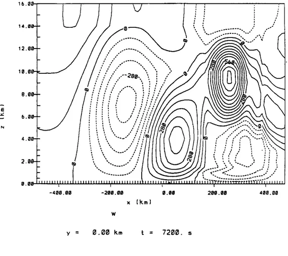
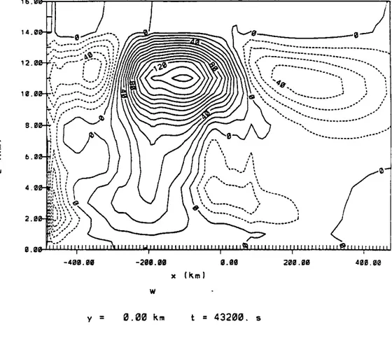
-40"."0 -2"111.0" 0.01 201.11 4Be.00 x Ikml w y 0.00 km 7200. s

Figure 3.6: (a) Two hour model simulation of vertical velocity to with cold low-level and warm high-level initial perturbation.

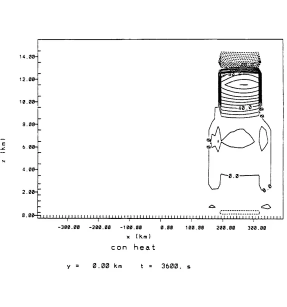
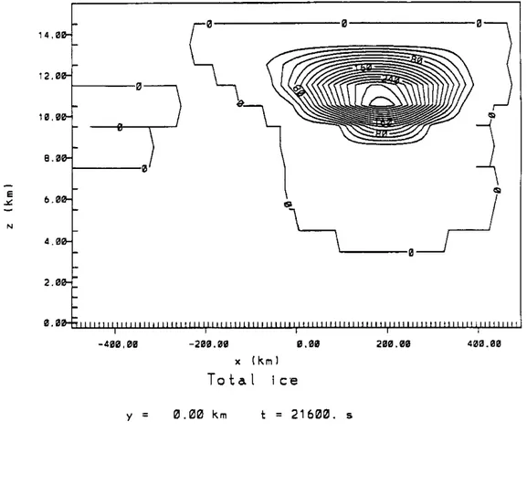
However, the low-level warm and upper-level cold initial baroclinic perturbation re-sults in a more persistent feature. The buoyancy force is quite large and strong ascent associated with the heating over the ocean occurs after one hour of model simulation (Fig. 3.7a). A large amount of heating (nearly 110 K day-I) is released between the heights of 8 and 13 km. Although this heating is large, it is necessary for the modelled atmosphere to maintain the disturbed cloud cluster. One hour after this heat warms the air, upward motion occurs over the ocean in that region (Fig. 3.7b). The maximum vertical velocity appears between 10 to 12 km above the sea level. The disturbed system, which has a positive relative vorticity of a magnitude of 0.13x10· s-l, includes partly convective (central area of the cloud cluster) and partly stratiform (front and rear of the cloud cluster) clouds that can be distinguished both from cloud water content and the updraft motion within the area. The maximum ice content in the cloud cluster is between 8 to 10 km. A portion of the anvil ice is spread westerly by the high-level easterly flow. This appears to represent a mesoscale convective system as well as one can in two dimen-sions. Therefore, this form of a perturbation disturbance seems more reasonable than the former one and each of the following simulations have used this initial disturbance.

3.2 Development Stage

After the initial disturbance is inserted in the model, the sinlulated cloud cluster develops over the ocean due to the lifting of the low-level air as condensation occurred above the 4 km height. Precipitation does not appear over the ocean until 3 hours of simulation (0700 LST). Rainfall is produced from sinlulated mesoscale cumulus with a 1.5 g kg-1 _{cloud water mixing ratio and lasts about one hour. The top of the cloud reaches}

about 12.5 km and the anvil around the cloud top stretches 180 km to the west from the main cloud cluster. The upper-level easterly wind forces the cloud cluster to propagate west. Meanwhile, a large amount of moisture from the evaporation over the ocean forms in front of the cloud cluster while it propagates westerly.

About two hours after sunrise (0800-0900 LST), the latent heat fluxes from the ocean are about nine times larger than those from the inland surface. However, at 1000 LST,

-

E ..: N -408. "" y -211.11 w 0.00 ~m 1.11 200.1118 400.00 x (~ml t • 43200. 5

Figure 3.6: (b) Twelve hour model simulation of vertical velocity w with cold low-level a.nd warm high-level initial perturbation.

E L N -32121.0'0 -22113.111111 -'''''.0'' B."" Hle.00 2121111.210 3'210.130 x I km I con heat y ~.~~ km t = 36~0. s

14 '2

,.

B

..

~

o ..

~

E

""

b N 4 2

..

-40111,0111 -2 ••.•• 121.1211 212111l,I!IB 4121111.0" x I km I w y 72"''''. $

04.3 12.3 13.21 8.0 e b .• .z: N 4.0 2.0 0.0 --- _____________ - 2 . ~~ ---__

---_ _

___

_

____ ::: :::::::: ::: ::_? __

~ _r~~~~:[~~-i:~:iii~-~H~::::::

::

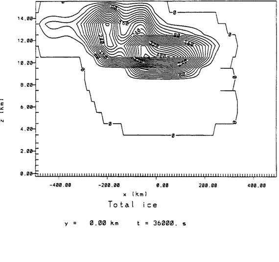
-:::::::::::::::::::::::::::::::::::::::::::::::-:;;-:-:-:;-:;;-:;:-:::::::::::~~~~~~~~~~~~~~~~~~~~~~~~~~:~::~:-y - : .. .-..•.••. _--- --::::;~ -~~::::::: -200.00 0,00 x IkmJ vir-pot-temp-per 0,00 km t = 21600, s 233.2113 431:1,321

Figure 3.8: (b) Control run at 1000 LST for virtual potential temperature perturbation

N

y

x I km)

Total ic'e

~.~~ km t = 2 1 6~~. 5

tens of em s-1 moves near the coast at 1100 1ST, the average latent heat fluxes overland increases to almost 600 W m-2 _{(Fig. 3.9) although the sensible heat flux is not that large}

because of the high soil moisture. In addition, the increase of the boundary layer mixing

-"

-55. -85, -116 ~ ::; -IU X ::; ... -178 ;: -20e ~ x -237

"

-

-267. ~ 0 -liP

"

::c -327 -358 -J88 -411. -441. -47fi -~Oll -531. -511 -5QQ.

Latent and Sensible Heat of Can Exp .

... '

,--

...

"

'1 I

,'

'

..

-'"

\\ _{I , I} l" _I I I I I I , I I , I

\ ..

I

I ' I

\ ..

I

I ' I I I I

I

\ I I I I

I

,

•

• •

,

I I I I • I I \ I I

I

I I \ I I I I I I ' I I ' I I _I ' _{, I} I \ , I \ • I \ • I \,1

't/

_,

, ,

_,

_.

,

•

.

•

,

_{, ,}

,

• ,

.

_,

,

" •

,

,

• •

,

•

•

• - - SeM;1N ... t an lei""

... Lot ... 1 Moat on lalld

... - - - Ulito'll " - I 0 " _ "

I. 10. 12. 14. 16. 18 20. 22. 2~

Local Time (hour)

Figure 3.9: Variation of averaged sensible and latent heat flux over land and ocean of the control run against time.

process over land at high sun angle transfers more low-level moist static energy higher into the atmosphere. Furthermore, the warmed air over the land is brought toward the ocean by the low-level westerly flow and the mesoscale convection is promoted over the ocean adjacent to the land.

New convection occurs in the region where warm air from the land converges with the cold flow in front of the cloud cluster. The maximum convective heating rate reaches about 9.5 K day-l at a height of around 10 km. This warmed air due to latent heat released from the convection, initiates the upward motion in front of the old cloud cluster

A mesoscale convective system develops over land at 1200 LST due to the increase of incoming solar radiation and greater land surface evaporation. The maximum convective heating rate within the convective system reaches a value of 80 K day-l at 1300 LST. The convective cloud top, indicated by a convective cooling rate of 100 K day-l, reaches to about 16 km. The maximum cloud water mixing ratio within the cloud cluster is 1.2 g kg-l at a height of 1.25 km near the coast. The cloud cluster consists of a major stratiform over the ocean and cumulus over both the land and ocean in front of it. Figure 3.10a gives the convective heating rate at 1300 LST.

By about 1300 LST there is a small amount of land precipitation far from the coast that is spread inland by the high-level easterly flow. The vertical velocity field (Fig. 3.lOb) shows that there is a weak downdraft to the west of the updraft at the high level. However, most of the rain droplets associated with the downdraft beneath the anvil evaporate before they reach the surface. Therefore, there is only minor precipitation recorded on the ground about 200 km west of the coastline. This anvil rainfall lasts about two hours.

Figure 3.11a-c depicts the vertical velocity, convective heating, and total ice content at 1400 LST. The vertical velocity exhibits two major upward motion centers. One is from the old cloud cluster while it moves inland. Another one, which forms over the land adjacent to the coast, is from local convection due to moist ascending air lifted by the release of sensible and latent heat fluxes to the atmosphere from the heated land surface. The ratio oflatent heat fluxes to the sensible heat fluxes over land is about 100-500 during most of the daytime because of high soil moisture loss (maximum 40% from the initial value) from the land. It is apparent that the existence of the local mesoscale convective system promotes the further development of the landfalling cloud cluster.

E

...

N :'~~-'" _" 14. '----.-12.

Ol

10.

'"

'"

8.

.

.

4. .0 2. 0 -411.21" y

'"

'"

'"

LJ

-211.1" x I km' con heat

'"m

_'"

~

ill

Q 21.0' 0.00 km t = 32400. s 280.ae _4211.""

e -'" N 12.'" 11.0 8.01

0-\.----2.0 1 . Ig.J.IJJJJWoI.J,W.lJ..UUJJ.JJ..U.w:tl!iIH -411 .• " -211.01 1.01 211.11 411.11 x Ikml w y ~.~~ km 324~~. s

'b. 14. 12. '0. 8. E -'" _b. N 4. 2. -40".eil -2 ••. 0.

_••••

x {km I w y ~.00 km t = 36~00. 5 20 •. 00 f ( ... ---\ :

-\

\ t, .:::::: ... ~. "'. ' ..

-" "---430.00

E .L N 14. 12. 18. B.

..

4. 2. ..."".. e, -4111"."1 y = -2ee,00 x I km I con heat

B.""

0.00 km t = 361210121. s 200,00 400."0

E -'" N -40ta,00 y -200.00 0.00 x I km J Total ice 0.00 km t = 36000. s 200.00 490.00

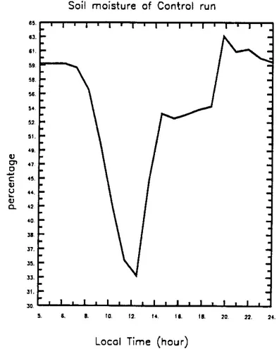
hundreds of kilometers from the coastline since the early morning due to the evapora.tion from the ground surface (Fig. 3.12). However, the soil tempera.ture near the coastline does not vary much due to reduction of the incoming solar radia.tion by the cloud.

Soil moisture of Control run

"

"1--...

..

eu

'"

"

o

-

C 4!S. eu ~ 4 •. eu c. .,

"

,.

l7. JO. ll. JI.

"

_{.. ..}

I. la, 12. '4. II. II. 1D. 22, 24,

Local Time (hour)

Figure 3.12: The varia.tion of the soil moisture with time of the control run a.t 100 west of the coastline.

By 1600 LST, a.n a.pparent upward motion associa.ted with the la.ndfa.lling mesoscale cloud cluster forms over the la.nd. The maximum upward motion center is loca.ted between

10 to 12 km (Fig. 3.13a). The upper-level easterly wind forms a strong vertical shear

in front of the cloud cluster between those levels (Fig. 3.13b). The upward motion is apparent and new mesoscale convection with a maximum heating rate of 14 K day-l at the 8 km height appears at about 250 km west of the coast. However, precipitation occurs over a wide region that includes 100 km over the ocean and 300 km over the land although the magnitudes are small (Fig. 3.14). The large area ofrainfall is the result of both stratiform and convective cloud precipitation. For stratiform rainfall, the precipitation particles in the upper portion of the anvil cloud are initially in the form of ice particles which grow as they descend until they melt below the O°C level and then partially evaporate while falling as rain droplets through unsaturated air below the base of the anvil in the cloud cluster. The stratiform rain associated with the mesoscale downdraft usually fall in the central and rear part of the cloud cluster. The convective showers, however, come from the melting of the ice particles and the super-cooled water droplets at the top and middle portion of the convective towers. The maximum cloud water mixing ratio is 1.2 g kg-1 over the land and 1.3 g kg-lover the ocean at this time.

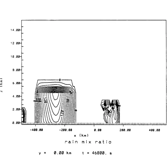
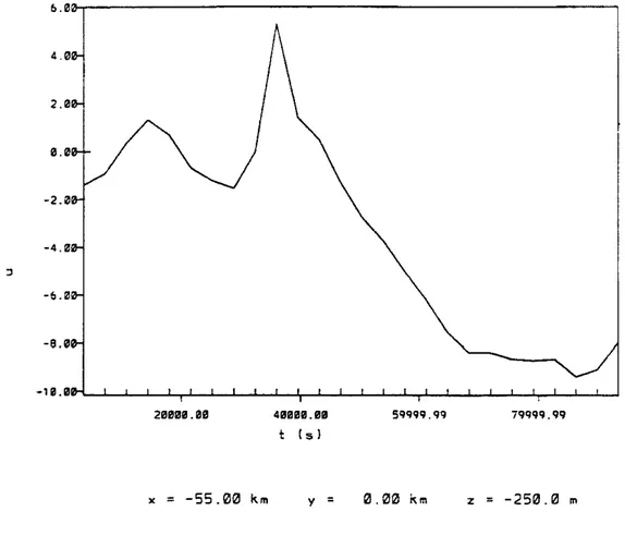
One hour later (1700 LST), the rainfall increases and covers the region between 100 to 400 km west of the coastline. Most of the rainfall at this time comes from the front of the cloud cluster. Figure 3.15 represents the rain mixing ratio at this time. The heavy rainfall at the leading edge of the cloud cluster is similar to the tropic squall line convection cloud clusters demonstrated by Houze (1982) with respect to the low-level outflow and the mesoscale rainfall features. Therefore, the easterly flow in the surface layer increases after the original cloud cluster moves inland. This flow transports moist air in the lower boundary layer from the ocean surface to supply the convective system over the land. Figure 3.16 gives the variation of the west-east component as a function of time at 250 m above the ground and 50 km west of the coastline. The increase of the low-level easterly wind is signincant since the cloud cluster has moved inland.

Three hours later (2000 LST), a warm and wet layer with a maximum cloud water mixing ratio of 1.9 g kg-1 and a

+

1.2°C virtual potential temperature perturbation forms around 4-5 km above sea level and extends 200 km over land and 200 km over the ocean,

-'11.11 -211.al 8.11 281.11 '11.11

x (km) w

y 0.00 km t = 43200. s

2 '~"'I8 . 0 0

-F

8.~0 B.0 -41110.1110 -20/11,1/10 u y ~.0111 km ~.~

••

0.B0 x (km I 4320111. s 200.1!10 ~.~ 8.~~ <: 41110.00

Precipitation at 1700 LST 20

"

I.. ~ .r.

,

.

... E E _1.2 ~ c: 0 :;:; _1.0 e

-.0.

·u

_0.'

"

~ a. 0.' 0.' 0.2 0.0 1LI.L&.IJL&.IJL&.IJLUJLUJi&.LIi&.LIi&.LI..u. ....

w.w.w.w.w.ul.ow..w...u

-47-4J.-Jil.-X--12 __ H._n._2I._1I._14._IL -7 -1 -0. 1. 7_ let 14. 17. 21 a

Location (km)

14 '2 10. S. E L- b.

,

,

. 2.

-4130.0" -2BB.Be B.Be 2ae.aa 4210.210 x (km'

rain mix ra.tio

y 0.00 km t = 46800. s

2131"".0" x = -55.00 km 4"'H!lI.II t i s I y Sqqqq.qq 0.00 km z = -250.0 m

FIgure 3.16: Varia.tion of low level west-east wind u of the control run 50 kIn west of the coast against time.

respectively. This relatively moist and warm thin layer may be caused by latent and infrared radiative heating within the cloud that is associated with the mesoscale ascending motion. A certain amount of precipitation falls at 50 km east and 150 km west of the coastline. Figure 3.17a-b illustrates the I/~ and the rain mixing ratio at this time. The pattern ofrainfall and corresponding thermal structure (Fig. 3.17c) indicate that most of the rain comes from the stratiform cloud that existed in the rear of the cloud cluster. The new cloud is indicated by a significant "valley" at 4 km level in the I/e field over the land

and sea near the coast region. 3.3 Decayed Stage

By about 2200 LST (18 hours of simulation), the cloud cluster has been weakened considerably in terms of cumulus convection activity and mesoscale precipitation. This occurs because the inland propagation of the cloud cluster moves it into less favorable conditions. The moisture flux over the soil is lower than that over water. The boundary layer turbulent mixing process is reduced in the late evening because the buoyancy term is negligible and the shear production term is the only energy input to the lower atmosphere. Figure 3.18 shows the vertical velocity field at this time. The ascending motion, which is associated with a weak ascent, is apparent although the magnitudes are small. The sinking motion due to nocturnal radiative cooling dominates a wide portion of the domain. The total ice content in the cloud cluster has decreased from 0.72 g kg-1 at 2000 LST to 0.63 g kg-1 _{between the heights of 13 to 14 km (Fig. 3.19). This lower ice content indicates}

that the weak ascending motion and absence of deep cumulus convection cannot transfer significant amounts oflow-Ievel moist air to the upper level. Hence, the cloud cluster loses its energy source.

The evolution of the lower level east-west wind component also indicates the land-falling of the cloud cluster. Figure 3.20 represents the variation of the lower level east-west wind with time 100 km west of the coast. The wind varies greatly near 1500 m above the ground. The turbulent mixing process is significant at 1400 LST when the monsoon cloud cluster approaches the coast. However, the onshore flow at the levels below 500 m

E -'" N -4013.08 y ... <;:.::::::::::::::. -2SS.SS s.ss x Ikm) vir-pot-temp-per 0.00 km t = 57600. s 2SS.SS

_4"".""

Figure 3.17: (a) Virtual potential temperature perturbation (s:,) at 2000 LST ofthe control run.

14. 12. , 0. e. E -"

.

N 4. 2. -4e0.00 -200.00 O,00 200.00 43111.0" x (km J r a i n mix· rat i 0 y 0.00 km t = 57600. s

,10-5.0 321. 321. 321. 4.

010

-l.0 ,10- 37 2 :::'---31 2 . .-

-:----...

. '-- 312. . /

0~

--

_e .z:. 2.0 ~304. _{304. 304.-}

--

- 110-1.0

-110-_I-- 296. 296. 296. 0.0 " , " , " , " , " _-,-

.

"

.

"

.

"

.

"

, -481.1111 -200.01 Il.Iae 210.01 • (kin)

E~U

POT TEMP

y 0.00 km t • 57b00. 5

lb. 14. 12.

1.

8 E

""

..

N 4. 2 .

..

-400. '''' -200.1210 •. ee 200.00 400.08 x ! km J w y 0.00 km 64800. s

'4. '2. , 0. 8. E 6.

'"

N 4. 2. 0. -400.00 y = -200.00 0.00 x I km I Total ice ~.0~ km t = b48~~. s 200.00 4'UI.00

Figure 3.19: Total ice content of the control run at 2200 LST.

.500 lU7 lJ75 2112. ~ E 2250.

-..<: .~

"

I lll7 11:15

."

-.

-.

Low level U over lend

-l.

-

,

•

.

...

'

.

U (m/s)

...

,

.

- - - 0 1 0 0 ~~ ·----'40Cl.ST ••••••••• 'lao tSl

...

_.

.

•

_"

OJ

"

of about 4 km from late evening until early morning. Figure 3.21 represents the total precipitation over the land. About 80% of the rain fell from the cloud cluster before 2200

10.0 .0 '.0 '0 ~ E E _'.0 ... c: ~ '.0 .8 :§-u '.0

"

~ a. '.0 2.0

"

•

•

•

• • •

•

Precipitation of Control run

•

_•

•

_•

•

_•

...

.

....

'....

~

i

\\ ".

..

.

-24,*,,~ ... 'I no..JI"IC. .. • ... ,1'-' pta.

,.i

_,

.

.

..

,

•

•

•

• • • : I

i

\ "

,

,

..

.

.

,

:

..

,

,f

\ .... ..

_,

...

",

... .

: ... '

.

..

_'

... : .. -/ ,~

...

"~", Location (km)

Figure 3.21: Total rainfall of 16, 18, and 20 hour simulation in the control run.

LST. The maximum rainfall was concentrated in the region between 200 to ·300 km west of the coastline.

The current model simulation results suggest that rainfall over the east coast of the India subcontinent during the monsoon season is partly from the major cloud cluster in the monsoon depression and partly from the local convective clouds which interact with the landfalling cloud cluster. The distribution of the precipitation is very consistent with the observational data mentioned in Fig. 3.4. Actual observed 24 hour precipitation from OOZ 7 July to OOZ 8 July shows that the maximum rainfall is located from 200 to 300

km northwest of the Indian east coast. The recorded 24 hour precipitation indicates that the maximum value is 96 mm at about 250 km northwest of the coast. However, the magnitude of the stratiform and convective rainfall from the modelled result (11.8 mm) is less than that in the real world (Fig. 3.21). However, the observed maximum is a point value, whereas the simulated rainfall is an area-average. The simulated value is probably also too small because horizontal convergence in the second spatial dimension has not been included in these experiments.

The model simulation results are consistent with the observed landfalling monsoon cloud cluster. The effect of surface heat fluxes on the inland propagation and develop-ment of the monsoon cloud cluster is apparent in the model simulation. Webster (1983) suggested that the surface hydrological effects can aid the poleward movement of the monsoon through the evaporative cooling of the precipitation moistened ground. The modeled results show that the supply of sensible and latent heat from the ground to the air destabilizes the atmosphere before the cloud cluster moves inland. The development of mesoscale convective systems over the land then promotes further increase of the cloud cluster when it moves inland. There are some differences between the modelled results and the observational data with respects to magnitude of precipitation. These differences may be caused by the following reasons: (1) this is a two-dimensional model simulation. The lack of variations in the north-south direction makes the modelled system lose a portion of the vortex effect. This vortex effect influences the intensity and evolution of the de-pression system. (2) The two-dimensional simulation also loses a portion of the moisture convergence. This will make the modelled magnitude of the precipitation less than reality. (3) The topographic forcing effect is not included in the model simulations. There is only

system and the landfalling cloud cluster; and (4) the typical inner structure of the cloud cluster associated with the su=er monsoon.

In the following chapters the sensitivity of the simulated cloud cluster to surface characteristics will be presented and discussed.

SENSITIVITY EXPERIMENTS

In Chapter 3, the evolution of a simulated landfalling monsoon cloud cluster which formed over the ocean was discussed. This simulated cloud cluster, although differing in some details, is consistent with the major features of a mesoscale convective complex associated with the monsoon depression observed over the Bay of Bengal on July 7-8, 1979. The observed cloud cluster (Houze and Churchill, 1987) has the typical characteristics of the tropical cloud cluster as suggested by Houze and Hobbs (1982). The modelled cloud cluster also has a large anvil canopy near the tropopause. The cloud cluster tends to travel by a combination of translation and discrete propagation, wherein areas of cloud systematically form at the leading edge of the system. The influence of land surface evaporation on an intensification of the cloud cluster is significant.

There are two major geographic factors which influence the evolution of the mesoscale convective system: the water and the land surface. Shukla and Misra's (1977) study indicated that heavy rainfall on the Indian continent was related to a positive sea surface temperature (SST) anomaly of the Arabian Sea. As discussed in Section 1.4 and 1.5, the effect of landscape on the mesoscale weather system as well as the summer monsoon, is significant. Mooley and Shukla (1987) suggested that soil moisture influenced the ground heating which in turn determined the sensible heat flux and affected the generation and dissipation of heat lows. The soil moisture effects could, therefore, be as important as SST anomaly effects on the summer monsoon.

In this chapter, several experiments are designed to study influence ofland and ocean surface characteristics on the variation of the mesoscale convective system associated with the monsoon depression.

convection.

In an attempt to isolate the effects of soil moisture on the mesoscale convective system, the simulation in Chapter 3 is repeated with a variation of the soil moisture from 0.8 (relative wet land surface) to 0.3 (relative dry land surface). Everything else is identical to the control run.

Here, the evolution and propagation of the simulated cloud cluster over ground sur-faces with different soil moisture will be tracked. At 1200 LST, the vertical motion field in the two experiments is very similar in the two runs with the center of upward motion located at about the same place. Two hours later at 1400 LST (Fig. 4.1a-b), the SLM run which represents the dry land surface situation, has shifted the center of the simulation's upward motion toward the west. The maximum upward motion in both the SHM simu-lation, which represents the wet land surface situation, and in the control run, is located along the vertical axis at the leading edge of the cloud cluster.

Before landfalling, in the SHM run, the latent heat fluxes are about 3 to 4 times larger than in the SLM run. In the wet land surface run, the deep cloud develops at 1100 LST over the ocean near the coastline first. Then the clouds form over both the land and ocean adjacent to the coastline. However, in the SLM case, the deep cloud first appears only over the land near the coastline at 1100 LST. It then moves inland (Fig. 4.2a-b). The total ice mixing ratios in the cloud cluster also exhibit relatively large values in the SHM experiment (Fig. 4.3a.b). The maximum ice mixing ratio is 0.46 g kg-1 _{in the SHM}

run and 0.38 g kg-1 _{in the SLM run at 1400 LST. The cloud cluster in the SHM run has}

-

E -'" N lb,0~---r~----r--r-r---' -40121.00 -200.1210 0,00 200,0" x I km J w y 0.00 km 30000. 5 0 - - - 1

,

....

_---.:

...

---.-.

: ! \ t ..

\.

"" .' .' " ' "

-.-._----.-_.-4130.1210

-411.11 -211.11 1.11 211.11 411.11

x Ikml w

y 0.00 km t = 36000. s

N

L.~

-400.1210 y x (km ) con heat 0.00 0.00 km t = 36000. s 4121121.1210

o

N -401.10 -200.00 0.00 20111.00 400.01i! x Ikml con heat y 0.00 km t = 36'H210. 5

'4.0 12.0 lI!1.0 B." E b.0 -" •

'

.

"

2." 0.0 -4"".0111 y -200.00 x I km I Total ice 0.00 km = 36000. s 200,01/1

Figure 4.3: (a) Total ice at 1400 LST for SHM case.

e -" -400."0 y -200.00 x (km I Total ice

0.""

0.00 km t = 36000. s 200.00

Figure 4.3: (b) Total ice at 1400 LST for SLM case.

Precipitation begins at 1300 LST in the SHM simulation. Rainfall from the stratiform cloud in the landfalling monsoon cloud cluster and the cloud cluster in front occurs first in the inland region, then in the coastline area. Minor precipitation well inland at this time indicates that the upper-level easterly flow spreads the anvil inland. However, there is no precipitation until 1600 LST in the SLM run. Rainfall in the SLM run is concentrated in a narrow inland range when it starts. The region near the coastline never gets any precipitation. It seems that most of the rainfall is from the local convective system which propagates westerly over the dry land. The cloud cluster itself, however, does not bring much precipitation at least when it inltially moves over the dry land.

Figure 4.4a-c give the comparison of the total precipitation at different times in the SLM, SHM, and control runs, respectively. The figures show that the simulated cloud cluster obtains more moist static energy from the wetter land surface. Therefore, local convection can more easily develop and the greater locally forced deep convection within the wetter monsoon cloud cluster in turn results in a large amount of rainfall over the land.

Furthermore, the dynamics of the convective systems are different in the two wet ground simulations. The system in the dry soil run does not become as focused as it is in the wetter soil case. The cloud cluster in the dry soil situation exhibits a more inland upward motion center at 1600 LST. The maximum upward motion at 1600 LST in the dry soil run at 11 km is 17 em s-1 while it is 13.1 em s-1 in the moist soil run. The convective activity lasts until 2100 LST in the wet land simulation. However, the upward motion center disappears after 1800 LST in the SLM run. This comparison indicates that the high low-level moist static energy over land associated with relatively moist soil greatly promotes the mesoscale convection not only of the landfalling monsoon cloud cluster but also the concurrent local convection.

4.2 The Influence of Surface Roughness

Previous discussions (Section 4.1) suggest that the low-level thermal and moisture supply over land is an important factor in influencing the variation of cloud cluster struc-ture and its precipitation pattern. Another possible factor influencing the intensity of the

~ E E ~ c: 0 :;: .8 '0. '0

.,

~ 0-I.'

'.,

...

...

"

'.'

,.,

2.'

"

'.1

,.,

,-,

'

·

"

·

,

·

,

•

•

·

, ,

..,.-

....

:

,

l ... .

.

,

I

f\

!

: \

I

_•

f

•

•

,

•

_•

•

_•

•

_•

•

_•

,

•

_•

•

_•

•

_•

•

_•

•

_•

•

_•

•

_•

•

• - - . - SfwIo . . . .. ••••••• SIm..., -.7-.'.-lt.-.M.-12.-a.-25.-2t.-II.-14,-IL _1. -1 -0. l. 7. 10. 14 17. 21. 25. Location (km)

~ E E ~ c: .9 .3

:§-u

"

~ a.

"

"

'.l

••

••

l.'

"

••

o.

0.0

l8-hour Total precipitation

...

.

'

,-:0°

/

_• • •

•

•

·

• ,-,

.

,

.

, _,

,

•

_•

• • _• •

_•

• _• • _• • _• • _•

•

_• •

·

•

_•

•

_• - C o n ..... ... .. SPom . .." . .....

""'--47-4l-J'-lI.-32,_2t __ ~._21_" ._I •. _1I _, -3 -0. 3. 7. 10 I. 17 21. 2!1. Location (km)