A Study on the Low Volatility Anomaly in the Swedish Stock Exchange Market: Modern Portfolio Theory

(1)

Höstterminen 2016 | LIU-IEI-FIL-G--16/01632--SE

A Study on the Low Volatility

Anomaly in the Swedish

Stock Exchange Market

– Modern Portfolio Theory

George Abo Al Ahad Denis Gerzic

Handledare: Göran Hägg Examinator: Peter Andersson

Linköpings universitet SE-581 83 Linköping, Sweden 013-28 10 00, www.liu.se

(2)

Abstract

This study investigates, with a critical approach, if portfolios consisting of high beta stocks yields more than portfolios consisting of low beta stocks in the Swedish stock exchange market. The chosen period is 1999-2016, covering both the Dot-Com Bubble and the financial crisis of 2008. We also investigate if the Capital Asset Pricing Model is valid by doing a test similar to Fama and Macbeth’s of 1973.

Based on earlier studies in the field and our own study we come to the conclusion that high beta stocks does not outperform low beta stocks in the Swedish stock market 1999-2016. We believe that this relationship arises from inefficiencies in the market and irrational investing. By doing this study we observe that, the use of beta as the only risk factor for explaining expected returns on stocks or portfolios is not correct.

(3)

Acknowledgements

Thanks to G ¨oran H¨agg, our mentor who helped us form this thesis. Our families who always support us.

(4)

Chapter 1 Introduction

The Capital Asset Pricing Model of Sharpe, Lintner and Black has for a long time shaped investors’ view of expected returns and risk. The model hold only one risk factor, the market portfolio1 and the expected return of a portfolio is given by the following relation:

E(_erp) =rf +βp(E(erm) −rf) (1.1) The essence of the model is that the market portfolio is mean-variance efficient in terms of the theory established by Harry Markowits in 1959. The efficiency of the market portfolio implies that expected returns on assets depend linearly on the risk measure, the market beta. In 1973 an empirical test of the CAPM was made by Fama and Macbeth (1973) using American financial data from 1926 to 1968. From the study they concluded that the hypothesis of the two parameter model, that the pricing of assets reflect the attempts of risk-averse investors to hold ef-ficient portfolios2 could not be rejected. Although the great impact of CAPM on the financial theory and Fama and Macbeths (1973) conclusions there have been several empirical contradictions of the Sharpe-Lintner-Black (SLB) model. Study-ing portfolios with high and low market betas has shown that the latter, has sur-prisingly produced higher risk-adjusted return over time. This phenomenon is known as the low volatility anomaly3. A famous contradiction to the theory is a study made by N. Baker and A. Haugen in 2011 where they by sorting stocks listed on the New York Stock Exchange by capitalization size and beta saw that the relation between beta and return became linearly negative. (Haugen, Robert. 2000)

Since the time of the study the world has gone through rapid technological de-velopment that has facilitated financial transactions leading to an expansion of the financial markets. Technology has also introduced high-frequency trading that is affecting market prices. Furthermore in recent years since the Dot-Com Bubble of 2000 and financial crisis of 2008 the world has experienced economic turbulence leading to abnormal economic conditions, such as negative interest

1_{The market portfolio is the portfolio containing all the capital assets in the world.}

2_{An efficient portfolio is a portfolio matching the preferences of a risk averse investor. That}

is that gives the highest expected return given level of risk or reversely, the lowest risk given a certain level of expected return.

(6)

rates, that puts existing models to test. Therefore it is in this study’s interest to investigate whether CAPM holds or not and consequently if high beta stocks has yielded more than low beta stocks under these conditions in the Swedish stock market. The test will be similar to the one made by Haugen and Baker but only beta is of interest, therefor sorting stocks in portfolios only as per their beta.

1.1 Objective

The objective of this study is to, with a critical approach, investigate if portfolios consisting of high beta stocks yields more than portfolios consisting of low beta stocks in the Swedish stock exchange market through 1999-2016. Furthermore the study will investigate if the Capital Asset Pricing Model is valid. The model will be tested on four different periods throughout 1999-2016. Two of the periods will cover the crises and the two others will be placed after the crises. The study will be carried out in the same fashion as Fama and Macbeth’s study of 1973 but using a different sorting-algorithm, more recent data and data from another market.

1.2 Hypothesis

The hypotheses to be verified or rejected in this study are as followed:

H1 Portfolios consisting of high beta stocks has yielded more than portfolios consisting of low beta stocks in the Swedish market 1999-2016.

H2 The CAPM has been valid for stocks listed on the Stockholm Exchange from 1999 - 2016.

1.3 Research Questions

This study will relate to a few questions that will be answered hereafter.

• Does the basic criterions of the CAPM hold in the Swedish stock market for the period 1999 - 2016?

• Has portfolios consisting of high beta stocks yielded more historically than portfolios consisting of low beta stocks?

• If the hypothesis H1 is rejected, what can the better performance of low beta portfolios relative to high beta portfolios be explained by?

(7)

1.4 Delimitation

The study will be conducted on data from the Swedish market only and will be compared with relevant studies in other countries. Moreover it will solely rely on theories within the framework of modern portfolio theory. To get statistical significance in the tests all the companies with a minimum of 10 years of historical data will be part of the analysis. Only the outcome of the t-test along with its hypothesis test at a significance level of 10-20% will determine whether H2 will be rejected or not4. More specifically the outcome is determined by the pattern and magnitudes of the t-statistics along with the results of the hypothesis tests of the t-tests.

(8)

Chapter 2 Research Overview

2.1 The Capital Asset Pricing Model

In the Capital Asset Pricing Model (CAPM) developed by Sharpe, Litner and Black (1972) investors are solely compensated for exposure to market risk mea-sured by the market portfolio1. The model will calculate the expected return of an investment in capital assets. The expected return of an arbitrary portfolio p is calculated through the following relation (Amenc, Noel; Le Sourde, Veronique. 2003): E(Re_p) = r_f +β_p(E(Re_m) −r_f) (2.1) βi = cov(Rep_t, eR_M_t) var(Re_M_t) (2.2) E(Re_p): is the expected return of the portfolio.2

βp: is the portfolio beta which measures the exposure to the one risk factor of

model, the market portfolio.

E(Rem): is the expected return from the market portfolio. rf: represent the risk-free rate.3

The model was developed under assumptions that are not always consistent with the ways of the real world. Therefore it is essential to bare these assumptions in mind when pricing asset and judging what to expect when using the model. All of the assumptions are included below (Amenc, Noel; Le Sourde, Veronique. 2003):

a) The probability distributions for portfolio returns are all normally distributed. b) All investors consider one and the same investment period and plan their

investments over that period.

1_{The market portfolio is the portfolio consisting of all capital assets in the world.} 2_∼_{is used to denote a stochastic variable.}

3_{The risk-free rate represents the interest an investor would expect from a risk-free investment}

over a given time period. This could for instance be the interest of a treasury bond of a financially stable country.

(9)

c) Investors are risk averse and seek to maximise the expected utility of their wealth at the end of the period.

d) When choosing their portfolios, investors only consider the first two mo-ments of return distribution: the expected return and the variance.

e) Investors have a limitless capacity to borrow and lend at the risk-free rate. f) Information is accessible cost-free and is available simultaneously to all

in-vestors.

g) All investors agree on the expected return, variance and covariance for all assets.

h) Markets are perfect, meaning there are no taxes and no transaction costs. All assets are traded and are infinitely divisible.

2.2 Low volatility anomaly

The empirical fact that low volatility stocks have higher expected returns is a anomaly in the financial world. This is quite remarkable since it speaks against the very essence of investing: that higher risk assets is expected to yield more. During the 1960’s and early 1970’s the standard approach for predicting the mean-variance efficiency of the market portfolio was the Capital Asset Pricing Model. Professional investors were convinced to invest largely in equity indexes that served as a representation of the market portfolio like the S&P 500. But as the low volatility anomaly increased investors started looking for more efficient in-vestments in the mean-variance method. (Baker, Nardin L. and Haugen, Robert A. 2012)

2.2.1 Size Effect

Another explanation of the low volatility anomaly and contradiction of the CAPM was covered by Banz (1981). Banz showed that the stocks of firms with low mar-ket capitalization’s have higher average returns than large-cap stocks. He also argues that market equity is a explanatory factor of the cross-section for average returns given by market betas.

2.2.2 Fama and French

In 1992, Fama and French made an analysis for the past 40 years to study the relationship between return and volatility. Fama and French sampled the the stocks listed in the NYSE index4. They found out that the claim which says that the stocks with higher market beta could be expected to result in higher returns has not been accurate. They could see that the linear relationship between the average return and market beta plainly presented negative slope after grouping

4_{NYSE is an index that measures the performance of all stocks listed on the New York Stock}

(10)

companies by size and risk. Instead they found that you can get a higher expected return from stocks that were cheap in terms of book value to stock price or earn-ings per share to stock price. i.e stocks that have low values on these ratios. They based their discovery on the assumption that cheap stocks have a tendency to not be profitable because they are in financial distress and accordingly they carry a larger risk regardless of its beta. As a consequence of this investors require higher return from these stocks. (Fama, E. F.; French, K. R. 1992)

The univariate relations between book to market equity, E/P, size, leverage and average return are strong compared to the relation between average return and beta. It is shown in multivariate tests that the relation between average return and size is negative and also robust to the inclusion of alternative variables. The relation between average return and book to market equity is positive and will also maintain in competition with alternative variables. Further, book to market equity has a consistently stronger role in average returns although the size effect has drawn more attention. (Fama, E. F.; French, K. R. 1992)

Three-Factor Model

Their conclusions has lead to the well known three-factor model. The model con-siders three key factors: firm size, book-to-market values and excess return on the market. In other words, the used factors are the spread in returns between small cap firms and large cap firms (SMB), spread between value and growth stocks (HML) and lastly the same market risk premium described in the CAPM.

r=rf +βm(Rm−rf) +bsSMB+bvHML (2.3)

Fama and French’s three factor model explains over 90% of the diversified port-folios returns. (Fama, E. F.; French, K. R. 1992)

Five-Factor Model

In 2015, Fama and French extended their model by adding further two factors: profitability and investment. The profitability factor (RMW) is the difference be-tween the returns of firms with robust and weak operating profitability. The in-vestment factor (CMA) is the difference between the returns of firms that invest defensively and firms that invest aggressively. In the US from 1963 to 2013, by adding RMW and CMA makes the HML factors needless since the time series of HML returns are completely explained by the other four factors. (Fama, E. F.; French, K. R. 2015).

Survivorship Bias

Fama and French’s analysis ran in to criticism in 1995 by Kothari, Shanke and Sloan. Kothari, Shanke and Sloan stated that Fama and French had systematically

(11)

removed firms that defaulted during the sample period. Remark that Fama and French contended that the higher expected return of cheap stocks came from the higher risk arising from the firm being in financial distress. Therefore Fama and French’s method tend to bias up the historical performance of the cheap stocks. The financial firms were removed due to the high leverage normally used for the everyday activities in these firms. (Robert A. Haugen. 2001)

2.2.3 Baker and Haugen

The study of Baker and Haugen extended over the time period 1990 to 2011. They covered 12 emerging markets and 21 developed countries. Their intention was to make a procedure that was transparent and simple. Their samples included non-surviving companies and their database included 99.5% of the capitalization in each country.

They computed the volatility of total return for each company in each country over a 24 month period starting from the first month of 1990. They rank stocks by volatility in each country and formed them into deciles. Then for each decile in each month they calculate the total return. After that they continued in the same way for the rest of the 264 months in the sample.

Barker and Haugen provides evidence of great importance where they demon-strate that the intensity of analysts coverage is greater for more volatile stocks than less volatile stocks. They find this by studying the number of analysts pro-viding a sell, buy or hold commendation for each stock and a stock’s rank in terms of market capitalization. They also provide evidence for the relationship between volatility and news coverage. Barker and Haugen studies the number of stories appearing on the Dow Jones News Wire for each stock. Furthermore they see that volatile stocks are, in fact, covered more frequently by the media.

The three main points they find through their study is: (i) financial institutions hold more volatile stocks, (ii) analysts’ coverage is significantly greater for more volatile stocks, and (iii) news coverage is more intense for more volatile stocks. All the given evidence is equivalent with there hypothesis that agency issues are responsible for creating demand for volatile stocks, which results in their over-pricing and their production of inferior returns in the future. The managers who is working for the agency’s might figure that the stocks they are recommending are newsworthy but the fact that they are volatile may outrun their attention. Which in turn leads to a demand by professional investors and their clients for these high volatile stocks and this creates a overvalued price of volatile stocks and subjugates their future expected returns. (Baker, Nardin L. and Haugen, Robert A. 2012)

2.3 Empirical Notions of the Capital Asset Pricing Model

For CAPM beta is the only risk measure which contributes to the expected return. Fama and French explained that the ratios were representative of alternative risk

(12)

measures.

Perhaps strongest evidence against the CAPM is the success of the expected re-turn models. They use multiple factors profiling the company to predict future returns. Measures of risk including beta are among the least powerful predic-tors of future return in these models. Whereas measures of cheapness like for instance earning per share to stock price have greater importance. (Robert A. Haugen. 2001)

2.3.1 Rolls Critic

Richard Roll made a analysis of the validity of empirical tests on CAPM. This analysis has become famous and named as Rolls critics. Roll made two key state-ments in his critics against CAPM regarding the market portfolio (Roll, Richard. 1976):

i) The market portfolio is not observable, therefore the true risk premium of exposure to market risk can not fully be defined. The optimal market port-folio should contain of all existing assets in the world. Many of them can not be sampled because the data does not exist.

(13)

Chapter 3 Theory and Method

3.1 Testable Criterion of the CAPM

As these assumptions are very restricting it is interesting to study the sustain-ability and performance of the model in specific markets. This can be done by introducing a contradictory generalized model of stochastic returns that will test its characterizing implications. From (2.1) three testable implications can be iden-tified (Fama, E.F; MacBeth, J.D. 1973):

1) The expected return of an efficient portfolio and its risk is described by a linear relationship.

2) βi is a complete measure of risk of asset i in the market portfolio m. That is,

no other risk measure appears in (2.1).

3) Higher risk should be associated with higher expected return in a market of risk averse investors. That is[E(Re_m) −E(Re₀)]1 >0.

3.1.1 Identifying an Efficient Market Portfolio

To be able to verify the three conditions stated above, an efficient portfolio m needs to be identified. Under the assumptions that the capital market is perfect, all information is available at no cost for all investors, investors agree on the re-turn distribution of all assets and portfolios and that short selling2 is allowed, the efficient market portfolio is defined by the weights (Amenc, Noel; Le Sourde, Veronique. 2003):

xim ≡ total market capitalization o f asset i

total market capitalization o f all assets. (3.1)

3.1.2 A Contradictory Stochastic Model for Returns

As the equation to be tested above, namely (2.1), is given in terms of expected re-turns. It is convenient to introduce a stochastic model of returns that is as general

1_{The market risk premium, where E}₍

e R0)= rf

2_{Short selling means speculating that an asset will drop in price and therefore borrows a}

quan-tity of the asset, sell it on the market and then buy it back and returns it to the owner when the price is lower. This means that the portfolio weight, xipfor that asset will be negative.

(14)

as possible. The following generalization is suggested: e

R_i,t =eλ_0,t+eλ_1,tβ_i+λe_2,tβ2_i +eλ_3,tδ_i+e_i,t (3.2) The subscript t refers to time point t, such that eR_i,t is the one-period percentage return of security i from time point t-1 to t. (3.2) allows all variables with a tilde to vary stochastically from one period to another. The stochastic variable eλ1,t

represents the market risk premium described in (2.1). eλ2,t is included to test the

second condition, linearity with respect to beta and requires that E(eλ_2,t) = 0. δ_i represents idiosyncratic risk3 and condition 3 requires that E(eλ_3,t) = 0. The last term, e_i,t is assumed to be independent of all other stochastic variables and have zero mean. Moreover if all return distributions are normally distributed then the stochastic variables of (3.2) need to have a multivariate normal distribution. (Fama, E.F; MacBeth, J.D. 1973)

3.1.3 Conditions on the Parameters of the Regression

Market efficiency in combination with the condition about linearity requires that the time series’ non-linearity coefficient, eλ2,t, should have a expected value of

zero. Which means that the mean of the time series in question should be zero. Formally, it is stated that eλ2,t must be fair game4. In the same manner, market

efficiency requires that the non-beta risk coefficient, eλ3,t is a fair game and the

same goes for eλ1,t− [E(Re_m) −E(Re₀)]. (Fama, E.F; MacBeth, J.D. 1973)

Condition of Risk-free Borrowing and Lending

No information has yet been presented about eλ0,t in (3.2). Given that E(eλ_2,t) = E(eλ_3,t) = E(e_i,t) = 0 then from (2.1): E(eλ_0,t) = E(Re₀), i.e. the expected return of any risk-less security. Therefore in an efficient market eλ0,t−E(Re₀)is required to be a fair game. Adding the assumption that there is unrestricted risk-less bor-rowing and lending at the known rate Rf ,tthen the model ends up in the capital

asset pricing model of Sharpe, Lintner and Black and E(eλ_0,t) = R_{f ,t}. (Fama, E.F; MacBeth, J.D. 1973)

3.1.4 Testable Hypotheses

To summarize, given (2.1), (3.2) and what is stated in the paragraphs above, the three testable implications are translated in to three hypotheses to be tested in this study (Fama, E.F; MacBeth, J.D. 1973):

C1) E(eλ2,t) =0 (linearity)

C2) E(eλ_3,t) = 0 (no effect of non-β risk)

C3) E(eλ_1,t) = [E(Re_m) −E(Re₀)] >0 (Positive expected return-risk trade-off)

3_{Risk that is not associated with beta of asset or portfolio i}

4_{A fair game is an investment without a risk premium. That is, the mean of a stochastic}

vari-able considered to be a fair game is zero. A fair game is a zero-sum game where someone’s gain is another’s loss and therefor every investor must break even over a period of time.

(15)

3.1.5 Linear Time Series Regression and Cross-Sectional

Regres-sion

Both the βi of portfolios and the stochastic parameters of (3.2) can be estimated

by regressing the time series of the returns of the portfolio on the returns of the market portfolio. That is, for each portfolio, the data is fitted to a straight line of the following equation:

R_i,1 = αi+ ˆβp(E(Re_m) −R_f) +_ee_p,t (3.3) The cross-sectional regression is then carried out by using the estimated betas of each portfolio of (3.3) in which the explained variable5 is associated with one period or point in time. This way for each set of returns and betas in each time period one estimate of the lambdas of (3.2) is obtained thus creating a time series of estimated stochastic risk factors.

Notable is that if the regression, estimating the CAPM relation, would be carried out for individual assets it would lead to getting an error-in-variable. The con-sequence of an error-in-variable for CAPM is that it would tend to bias up alpha and bias down the market risk premium. (Blomvall, J ¨orgen. 2016)

3.2 Two tailed t-test of a Population’s Mean

Having the time series of the estimated lambdas. The two tailed t-test can be used to find out whether the sample has a certain hypothesised mean6 or if enough evidence is supplied to be able to reject that hypothesis. Thus the problem can formulated as such:

(

H0=µ =µ0

H1 =µ 6=µ0

H0is rejected when the mean of the sample analysed is far from the hypothesised.

The distance from the hypothesised mean is quantified by the t-statistic which is calculated in the following way:

t= x−µ0

s/√n

Where x is the sample mean, µ0is the hypothesised mean, s is the standard

devi-ation if of the sample and n is the sample size. Hence the t-statistic is a ratio of the deviation of an estimated parameter from its observed value and its standard er-ror. With other words the t-stat is a measure of how extreme a statistical estimate is. By looking at the equation it becomes clear that when the t-statistic is close to zero when the sample mean is close to the hypothesised one. A big negative or positive number would indicate that most values in the sample deviate largely from the mean value.

5_{The explained variable is the variable which is to be estimated.}

(16)

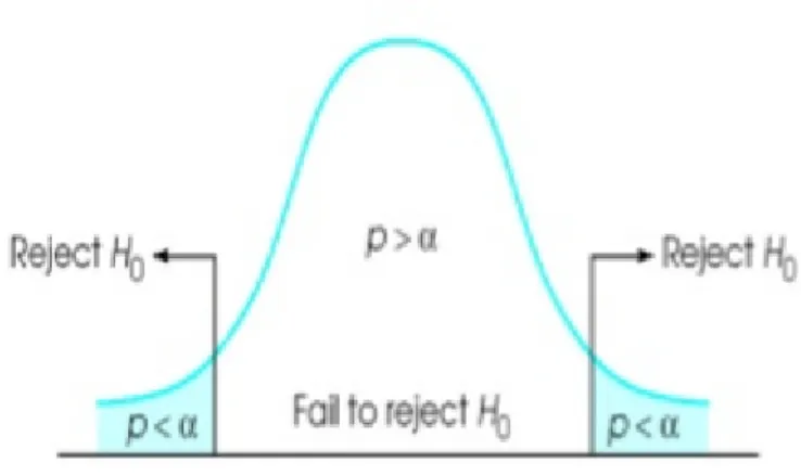
The calculated t-statistic resembles a random number in the student’s t-distribution and the t-statistics for which we accept or reject the null hypothesis are therefor given by the T-values as shown in Figure (3.1), which contains 1-α of the probabil-ity distribution with n-1 degrees of freedom. That is, there is a (1-α)*100% chance of our t value to end up in the interval of [-T,T]. Given that, if our t-statistic is outside this interval we can with great confidence say that we have enough evi-dence as to reject our null hypothesis, thus the sample mean is almost surly not the same as the hypothesised mean. Thus rejecting the null hypothesis in a big sample would be of evidence that our mean is different from the guessed mean where as accepting the null hypothesis could still mean that the true mean are relatively far away from the hypothesised mean. (Blom, Gunnar; Enger, Jan; En-glund,Gunnar; Grandell, Jan; Holst, Lars. 2005) In this study the level of signif-icance will be set to 10% which will contain 5% of the distribution in each tail. Therefore if most of the estimates ends up in that interval we can be confident in rejecting the null hypothesis.

Figure 3.1: Shows the student’s t-distribution, the T-values and the p-values for which we reject the null hypothesis.

3.3 Test of H1

To reach the objective of the study and the hypotheses stated in section 1.2 will be tested. To validate hypothesis H1 a study similar to the one Baker and Haugen did, described in chapter 2, will be conducted, except for sorting stock as per their size. This study will test whether high beta stocks historically has yielded more than low beta stocks during the whole period in question.

For both studies historical returns of 1095 stocks from the Swedish Stock Ex-change from 1995 - 2016 will be analysed. Out of these, the stocks that have less than 10 years of data will be excluded from the study. The time period is chosen so that the dot-com bubble of 2000 and the global financial crisis of 2008 are cov-ered. The information and financial data needed for the analysis will be extracted from the database of Thomson Reuters Eikon, Datastream and Bloomberg.

(17)

To test if high beta stocks yield more than low beta stocks historical stock prices including dividends are collected in a time series. Thereafter the returns for each asset in the sample is calculated. Having the returns for each asset, the exposure to the risk factor, βi can be calculated by regressing the previous 24-48 months

on the chosen risk factor, the Swedish SIX Portfolio Return Index. The regression for each asset will not be conducted if less than 24 months of data returns are available in that period. For each asset the regression is carried out by regressing the following data:

e

Ri,t =αi+ ˆβiRe_m+_ee_it (3.4) Where Ri,tis the return of asset i at time t, eRmis the market return, ˆβiis an

estima-tion of the true exposure of asset i to the market portfolio and α is an offset term that will not affect the slope (i.e. the beta) of the regression which is the objective of this regression. The index t represent each month in 1995 - 2016.

The first four years, 1995 - 1999 are used to get an initiating estimate of the port-folio betas. Those assets that meet the requirement of having at least 24 months of price information that period will be sorted in to ten different portfolios. Then each month of the whole the period the betas are re-estimated using a rolling win-dow of 48 months and assets are resorted into the different portfolios as per their beta that month.

How many assets that is placed into each portfolio is determined by the follow-ing: Let N be the total number of securities meeting the requirements each month and K the number of portfolios. Then in the middle portfolios int(N/K)7 securi-ties are placed and in the first and last portfolio if int(N/K) + 1/2(N - K·int(N/K)) is divisible by two, half of the remaining assets are placed in each portfolio, else the first portfolio get one asset more.

Next step is to calculate the total and expected returns for the K portfolios over the whole period. This will be done using logarithmic returns. When working with logarithmic returns, the total return of a portfolio is calculated as the sum of all returns and the mean resembles the expected return. Taking the natural number elevated with the calculated logarithmic return will give the arithmetic return in percent.

A representation of both expected and total portfolio returns versus portfolio be-tas, from where a conclusion of whether high beta stocks has yielded more than low beta stocks, will be presented in the analysis section.

3.4 Test of H2

The test that tests if CAPM holds or not uses the same sorting-algorithm as the previous test. This test will be done sorting assets in first 10 portfolios and then 20

(18)

portfolios. The test of model will be conducted on four different periods during 1999 - 2016 and these are:

1) Crisis period 1: January 1999 - January 2004. 2) Postcrisis period 2: January 2003 - January 2007. 3) Crisis period 2: January 2007 - January 2011. 4) Postcrisis period: January 2011 - January 2015.

Using the estimated betas of each portfolio the risk-premium of each risk-factor described in (3.2) can be estimated for the period. That is, each month of the pe-riod the following parameters are estimated: eλ0,t, eλ1,t, eλ2,t, eλ3,t. Having the time

series of these estimations the expected value of the time series represents the ex-pected risk premium of each factor. As chapter 2 states the exex-pected value of eλ2,t,

e

λ3,t and eλ0,t−Rf ,t, should be zero whereas the expected value of eλ1,t should be

greater than zero. The t-test will determine if they are zero or not.

Since the portfolio returns each month will be explained by the lambda param-eters using 10 portfolios i.e. four paramparam-eters are estimated using 10 data points which can give pour estimations. Therefor it is convenient to try the same model using 20 portfolios as-well. Using more portfolios leads to less assets in each portfolio which as mentioned in section 3.1.5 gives poorer estimation of the be-tas. That is there is a trade of between using using more portfolios and getting better estimation of the risk factors. Since 274 assets are included in the study the portfolio betas are believed to be relatively well estimated even when using 20 portfolios. The results of this regression will be presented in a separate table and will be analysed in relation to the results of the 10 portfolio regression.

Since in general when regressing over a larger time-series the standard error is minimized and therefor the explanatory variable becomes relatively large to the error. In this study this would mean that the exposure towards the idiosyncratic risk, δiis small. When carrying out the cross-sectional regression which estimates

the idiosyncratic risk premium i.e. λ3, will consequently tend to be big. Such

phenomenon can impair the results of the other variables. If this is the case for the Swedish data, a regression without the parameter eλ3,t, that will be

comple-mentary for the results of the complete regression, will be carried out. That is we try the same model under the assumption that the exposure towards eλ3,tis so

small that it can be omitted and thus we only check the linearity condition and if eλ0,t can resemble the risk free rate. These results will be presented in the same

tables under what will be called Panel B. This regression will be tested with the two tailed hypothesis test using a level of significance of 20% meaning that less room is given for accepting the null hypothesis and therefor accepting the null hypothesis is a stronger indication that the estimated mean is near zero.

(19)

Chapter 4 Results and Analysis

4.1 H1 Test

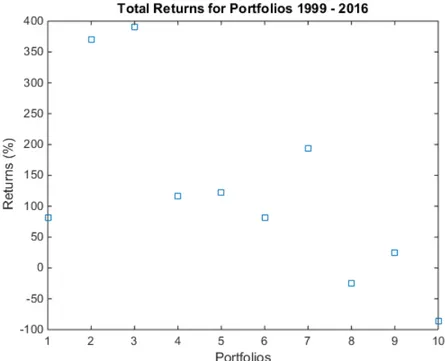
To control the H1 hypothesis all the returns for each portfolio was summarized for all of the 209 months. After that the mean of each portfolio was calculated to get a expected return for 209 months. Our results are pointing to the same find-ings made by Baker and Haugen in 2011, known as the low volatility anomaly. As seen in figure 4.1 high beta portfolios does not have a higher total return than lower beta portfolios during 1999 - 2016 and based on that the H1 hypothesis is rejected.

Figure 4.1: Total excess return of investment for each portfolio for the period: 1999-2016. Figure 4.1 displays the return of each portfolio. Portfolio 10 has the highest beta and portfolio 1 the lowest. From the Figure 4.1 we can see that portfolios with low- and mid-sized beta, has historically outperformed portfolios with higher beta in the Swedish stock market. We find this strange since we, according to CAPM, would expect an increasing return with increasing beta. This would mean

(20)

that we expect a somewhat increasing relationship moving to the right in the Fig-ure 4.1. The conclusion that can be made after this result is that the basic pillar of finance, the greater the risk the bigger the reward, does not apply in this case. More detailed key results from the calculations are shown in the tables below:

Portfolios: 1 2 3 4 5 6 7 8 9 10

Ave. yearly return 0.0353 0.0915 0.0939 0.0456 0.0471 0.0353 0.0635 -0.0163 0.128 -0.1169 Ave. assets 24.35 22.44 22.44 22.44 22.44 22.44 22.44 22.44 22.44 23.78 Ave. β -0.0137 0.3802 0.5359 0.6572 0.7746 0.8934 1.0179 1.1863 1.4309 2.0043

Table 4.1: Portfolios formed on beta size.

Furthermore reading from the Figure 4.1 and Table 4.1, it is interesting to notice a somewhat linearly decreasing relationship. We can see that the last portfolio con-sisting of the stocks with the highest beta with an average β of 2.0043, strangely has a negative expected and total return. This might be reasonable since the pe-riod of study cover both the dot-com bubble and the financial crisis of 2008 and some stocks have still not recovered from that chock. Portfolios 2 and 3, contain-ing an average β of 0.38 and 0.53, clearly yields most with respect to their beta value. Another interesting portfolio is number 7, having averaged with an beta of 1.0179 who yields the third most of the 10 portfolios.

Just as the discoveries of Fama and French in 1992 and Haugen and Baker in 2012, we can, based on our results, clearly reject the assertion that the stocks with higher market beta could be expected to yield more has not been accurate. From the results it is clear that the low volatility anomaly is still and if not even more present in the Swedish stock market 1999-2016. Holding assets from from portfo-lio 2-5 would clearly be more remunerating per unit beta than the other portfoportfo-lios with more systematically risky assets.

It is important to remark that Fama and French assumed that high leverage was a sign of a firm possibly being in financial distress. Therefor the financial firms were screened out in their study due to the high leverage normally used for the everyday activities in these firms. But using high leverage does not necessarily mean that a firm is in financial distress. High leverage could perfectly match the risk profile of a firm and therefor financial firms has not been screened out in this study. Even when including financial firms the essence of the results do not change.

As Fama and French’s study, our study also contain data with only surviving companies for the time period 1995-2016. However we did not removed de-faulted firms systematically. The reason for this outcome depends on lack of data. This bias could maybe affect the result and our test of the low volatility anomaly. But we know from the Barker and Haugen study, where they did include the not surviving stocks, that our results of the low volatility anomaly would not change. We have good reasons to believe that the same pattern persists. Since we did not have access to data including book to market equity, we can not demonstrate the impact book to market has for the average returns of the portfolios. But we still find there results interesting and does not judged out that it could be an impact of the factors the described in their study. The factors demonstrates the impact of

(21)

book to market equity and the risk premium arising from the size of the firm to explain the higher return for low beta portfolios.

According to Haugen and Baker, these factors does not necessary need to be risk-factors. Some of Haugen and Baker’s assumptions are that cross-sectional payoff to risk bearing is highly negative and the scariest (the most volatile) stock port-folios have the lowest expected returns. They also state that there is a negative relation when exposing to the risk factor. By looking at Figure 4.1 we see that we have same negative relation measuring risk in beta. This negative relation could be a result of the inefficient market, and also a result of the CAPM theory’s impact on the market. This leads to people getting stuck in the teaching that high risk stocks yields higher than low risk stocks. The assumptions therefor tend to drive up the prices for the volatile stocks, since many investors will buy these stocks ex-pecting a higher return while ignoring the low volatile stocks. Another possible reason for an inefficient market is the driving up of the volatility by indirect mar-keting via high news and analyst coverage. The high coverage tends to hype the volatile stocks and drive up their prices overvaluing them while undervaluing the low volatile stocks. These assumptions results in a wrong weighted supply and demand because the high risk stocks will be overvalued and low risk stocks will be undervalued. This will lead to the stocks not having the right expected returns and the CAPM will not prevail.

4.2 H2 Test

Table 4.2 to Table 4.5 contain much of information about what we can expect from each parameter of the regression of (2.4). Panel B presents the result of the regres-sion carried out under the assumption that the factor loading of the idiosyncratic risk, δi, is zero for all portfolios. The tables can tell us the magnitude of each

risk factor and if it is expected to contribute positively or negatively to the re-turn. Since we assume that the mean of each lambda population is zero when calculating the t-statistics, a number close to zero would mean that most our esti-mates each month are symmetrically distributed around zero. Therefor it is very likely that the expected value of that random variable would be zero. A large positive number on the other hand would mean that most of the estimates are distributed on the positive tail of the assumed normal distribution. This means that we would expect the random variable to have mainly positive outcomes. Implicitly a large negative number would indicate the contrary. We find it more convenient to rely on the results of the 20 portfolio test since they give better esti-mations of the lambda parameters. But we realize a common pattern in the signs of the mean values and t-stat and to some extent their relative size as well which could point to the same findings using either one of both tables.

Judging from Table 4.4 and Table 4.5 we cannot fully accept H2 in any of the periods studied. In all periods except 2003-07 the hypothesis tests shows that the C2 condition (no effect of non-β risk) is clearly rejected since we have large t-statical values. It is also safe to believe that even during 2003-07 we have a factor of idiosyncratic risk contributing to the returns since the mean value is relatively large to the other factors even there. The large expected values, λ3for all of the

(22)

periods can be explained by the small exposure to those risk factors i.e. s(_ee_i,t), that

are used in the regression, are on average very small. Realising the patterns in the signs, we see that all t-statistics are negative which is why we believe that if such a factor exists it would contribute negatively to the returns. But since we have very small exposure to the factor we deem it necessary to try the regression without it. That is we try the same model under the assumption that the exposure towards the risk factor is so small that it can be neglected. We can state this since having a portfolios consisting of many assets the idiosyncratic risk is diversified away since this factor arises from independent and identically distributed stochastic variables with zero mean, the idiosyncratic risk of a portfolio converges to zero as the number of assets in each portfolio increase. The results from that regression are presented in panel B and are complementary to the regression of panel A. As seen in Table 4.3 and Table 4.2, the results of the t-statistic and expected value of f

γ3even when using 10 portfolios which gives stronger ground to accept what is

previously stated. Period λ0 λ1 λ2 λ3 λ0−Ro Panel A 1999-04 0.0342 -0.0164 0.0063 -0.2471 0.0312 2003-07 0.0209 0.0136 -0.0036 -0.0572 0.0190 2007-11 0.0161 -0.0007 0.0000 -0.1951 0.0145 2011-15 0.0312 -0.0099 0.0065 -0.2562 0.0304 Panel B 1999-04 0.0126 -0.0171 0.0003 - 0.0096 2003-07 0.0155 0.0111 -0.0037 - 0.0136 2007-11 -0.0079 0.0114 -0.0069 - -0.0095 2011-15 -0.0052 0.0153 -0.0066 - -0.0060

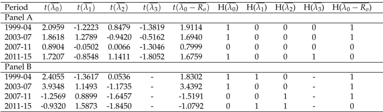
Table 4.2: Summary of the regression parameters of (2.4). The over-lining indicates the expected value of the stochastic variables, which is the mean value since they are assumed to be normally distributed. Period t(λ0) t(λ1) t(λ2) t(λ3) t(λ0− Ro) H(λ0) H(λ1) H(λ2) H(λ3) H(λ0− Ro) Panel A 1999-04 2.0959 -1.2223 0.8479 -1.3819 1.9114 1 0 0 0 1 2003-07 1.8618 1.2789 -0.9420 -0.5162 1.6940 1 0 0 0 1 2007-11 0.8904 -0.0502 0.0066 -1.3046 0.7999 0 0 0 0 0 2011-15 1.7207 -0.8548 1.1411 -1.8052 1.6759 1 0 0 1 0 Panel B 1999-04 2.4055 -1.3617 0.0536 - 1.8302 1 1 0 - 1 2003-07 3.9348 1.1493 -1.1735 - 3.4392 1 0 0 - 1 2007-11 -1.2569 0.8899 -1.6457 - -1.5191 0 0 1 - 1 2011-15 -0.9320 1.5873 -1.8450 - -1.0792 0 1 1 - 0

Table 4.3: Summary results for the t-tests of the risk factors at a level of significance of 10% for panel A and 20% for panel B using 10 portfolios. Hx = 1 means that there is

enough evidence as to reject the null hypothesis whereas Hx= 0 states the contrary.

Analysing the condition of positive expected return-risk trade i.e. E(eλ_1,t) = λ₁ > 0, we accept the hypothesis if this condition is on average fulfilled in all periods. In panel A of Table 4.3, we see that this condition is not fulfilled for the periods

(23)

1999-04, 2007-11 and 2011-15 and 1999-04 in panel B. Since most of t-statistics for

λ1 have a negative sign when looking to panel A, it indicates that the

hypothe-sised market risk premium is likely to be negative for the mentioned periods. On the other hand, looking to panel B of Table 4.3 and Table 4.5 the t-statistics are pos-itive in all periods except the Dot-Com crisis period of 1999-04. It is therefor hard to verify that we on average have a positive payoff between risk measured by beta and return. But Looking over both tables we notice that halve of t-statistics are positive and the ones that are negative have relatively small t-statistic values expect for 1999-04. Consequently there is enough indications that the market risk premium exists and is likely to contribute slightly positively to the returns over a longer period of time but could in certain periods affect the returns negatively as is seen in the results of the t-statistics year 1999-04.

Period λ0 λ1 λ2 λ3 λ0−Ro Panel A 1999-04 0.0256 -0.0182 0.0047 -0.1419 0.0226 2003-07 0.0200 0.0137 -0.0041 -0.0473 0.0182 2007-11 0.0248 -0.0075 0.0040 -0.2629 0.0231 2011-15 0.0282 -0.0021 0.0022 -0.2390 0.0274 Panel B 1999-04 0.0123 -0.0156 -0.0003 - 0.0092 2003-07 0.0155 0.0120 -0.0042 - 0.0137 2007-11 -0.0079 0.0114 -0.0071 - -0.0095 2011-15 -0.0053 0.0168 -0.0078 - -0.0062

Table 4.4: Summary of the regression parameters of (2.4) when using 20 portfolios. The over-lining indicates the expected value of the stochastic variables, which is the mean value since they are assumed to be normally distributed.

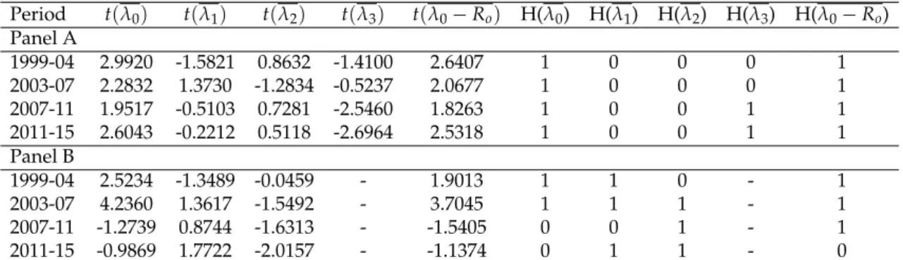
Period t(λ0) t(λ1) t(λ2) t(λ3) t(λ0−Ro) H(λ0) H(λ1) H(λ2) H(λ3) H(λ0−Ro) Panel A 1999-04 2.9920 -1.5821 0.8632 -1.4100 2.6407 1 0 0 0 1 2003-07 2.2832 1.3730 -1.2834 -0.5237 2.0677 1 0 0 0 1 2007-11 1.9517 -0.5103 0.7281 -2.5460 1.8263 1 0 0 1 1 2011-15 2.6043 -0.2212 0.5118 -2.6964 2.5318 1 0 0 1 1 Panel B 1999-04 2.5234 -1.3489 -0.0459 - 1.9013 1 1 0 - 1 2003-07 4.2360 1.3617 -1.5492 - 3.7045 1 1 1 - 1 2007-11 -1.2739 0.8744 -1.6313 - -1.5405 0 0 1 - 1 2011-15 -0.9869 1.7722 -2.0157 - -1.1374 0 1 1 - 0

Table 4.5: Summary results for the t-tests of the risk factors at a level of significance of 10% for panel A and 20% for panel B using 20 portfolios. Hx = 1 means that there is

enough evidence as to reject the null hypothesis whereas Hx = 0 states the contrary.

As for λ2, the hypothesis tests does not reject the hypothesis that E(eλ_2,t) = 0 in any of the periods. This does not directly mean that we are willing to accept the null hypothesis. We do accept it for any given period only if the t-statistics and mean values are close to zero. Looking at panel A of Table 4.3 and Table 4.5, the linearity condition C1 is likely to be fulfilled at least for the periods 1999-04 and

(24)

2007-11 and in panel B it seems to be full-filled for only 1999-04. This can be said since the t-statistics are reasonably small and looking to the expected value they are very small during those periods as well, which also indicates that it should be close to 0. Looking over both tables it is interesting to notice the pattern in the signs of the expected value of λ2 and the t-statistics. Since most of them are

negative and varying in size over the periods, we could expect this factor to con-tribute slightly and negatively to the returns or at least we cannot be as sure as to completely neglect its existence. Panel B in Table 4.3 states that the linearity condition is fulfilled only during 1999-04 and that we have enough evidence as to reject the null hypothesis during 2007-11 and 2011-15. Consequently we can-not fully accept the linearity condition C1 for any of the periods except 1999-04. Based on this it is hard to test whether E(eλ_0,t) = E(Re₀)since it requires that con-ditions C1-C3 is fulfilled. From the results of both tables it is very clear that it is not the risk free rate. But in panel B it is much closer to the risk free rate but still proportionally far away in all periods. We therefor reject the hypothesis that

λ0,t−Re₀ is a fair game. From the results obtained in panel B we realize that the importance of both λ0 and λ2 are biased up which is why we believe that it is

likely that other factors could be involved in the pricing of the assets.

In conclusion we cannot find any period where the linear relationship between the market beta and expected returns aren’t influenced by the other factors in-troduced in (2.4). Looking over all periods we have reasons to believe that the market beta affects the returns to some extent but that there are other factors that also are contributing to the returns each month. Moreover, we believe that hy-pothesis H2 can be rejected on the basis that we do not live in an world where the assumptions of the CAPM are fully true. For instance the efficient market hypothesis assumes that all information concerning a stock is available and is the same for all investors. This is not true since there exists information gaps that misprices stocks and creates arbitrage.

As trying to explain the higher return from low or mid sized beta portfolios we find the conclusions from Fama and French’s (1992) and Banz (1981) studies in-teresting. Their studies conclude that there is a premium arising from firm size and book-to-market equity. In our study it would be interesting to investigate the size of the companies in each portfolio over time. But due to lack of data about each companies market capitalization we couldn’t conduct such a test and therefor have a hard time verifying their findings.

4.2.1 Comments on the Approach

Have in mind that the SIX portfolio index was used as a proxy for the market in this study. This market portfolio is far away from being a portfolio consisting all the assets in the world. Therefor the calculated betas are merely estimates of the true betas but considered fairly estimated since SIX portfolio is the index which contain all the mid- and large-cap stocks traded at the Stockholm exchange mar-ket. The estimations can be called fair since in accordance with Roll’s critic to the CAPM, it is impossible to construct the perfect market portfolio. We believe

(25)

that the estimated betas at least points in the same direction as the true betas if looking to their the sign and relative size.

The idea with dividing stocks into beta-sized portfolios is used to minimize varia-tions in betas of assets within a portfolio. This method gives more accurate results since each portfolio will be represented by assets of the same risk class. Another reason for sorting portfolios as per their beta, is because choosing assets arbitrar-ily tends to give a beta around one since it have great chances of becoming well diversified when a great number of assets are added to it. Also by using port-folios rather than individual securities, we reduce the loss of information in the risk-return test. (Blume, E. Marshall. 1970)

When estimating beta there is a trade-off between using much data, leading to a high statistical significance or using less data and being able to detect a more uptodate correlation between market and stock or portfolio. Therefore a 24 -48 months period has been chosen when estimating the betas. Monthly data is used to correct the thin-trading problem in small stocks. This occurs because of non synchronous data, hence stocks do not trade at the same time due to illiquid trading. Monthly data are also used because it is empirically known to be more normal distributed than shorter time periods.

It is also important to remark that the two tailed test with the underlying assump-tion of respect to a normal distribuassump-tion can be conducted since the returns are assumed to be normally distributed which implies that the stochastic variables of (2.4) also must be normally distributed. Financial data is not perfectly normally distributed if we use daily data but gets more normally distributed using weekly and monthly data. Furthermore if CAPM have been fully valid in the Swedish stock market 1999 - 2016 and the SIX portfolio have resembled the market portfo-lio perfectly, our data would perfectly adapt to the CAPM relation and all excess variables of (2.4) would be zero. Since these assumptions are very stringent and not fully true the results, as seen in all tables, will deviate from what is stated by the model and we get non-zero expected value estimates of the stochastic vari-ables.

Furthermore the idea of using 20 portfolios is to get better statistical significance since we, each month, are trying to estimate four parameters using 10 data points when using 10 portfolios. Therefor we feel that it is necessary to observe the dif-ference of the results when using 20 portfolios instead of 10. One would think the more portfolios used the better the estimates of the four risk factors are. But as mentioned previously estimates of betas are better for portfolios than for individ-ual assets therefor the more assets we have in a portfolio the better the estimation of beta gets. Since the beta of each portfolio each month are inputs when esti-mating the risk factors, we have a trade of between the number of portfolios and how good we want our beta estimates to be. Comparing Table 4.3 and Table 4.5 we can see more logical estimates of what should resemble the risk free rate in the CAPM. When using 10 portfolios we have an monthly average return, from

λ0, between -3.45% and 5.91% which is very deviant from the risk free rate. The

(26)

therefor consider using 20 portfolios for the study a much better option.

The 3M Swedish treasury bill was used for the evaluation of the risk-free rate. First we used (5.1) to evaluate the effective rate on a yearly basis. Then we con-verted it to monthly effective rate by using (5.2). The risk-free rate is a theoretical concept. Hence it does not exist a risk-free investment in the real life, and it is of-ten used in CAPM. To work out the risk-free rate in a particular situation a bond considered risk-free will be used; Swedish Treasury Bill 3 Month.

rf = (1+ r3m 100 90 360) (365/90)₋ 1 (4.1) rf m = (rf +1)(30/365)−1 (4.2)

(27)

Chapter 5 Conclusion

Our study clearly indicates that portfolios with lower beta have historically given a higher return than portfolios with higher beta in the Swedish Stock Market. Furthermore, in base of the H2 test, we cannot establish that the CAPM solely explains the expected return of the portfolios. We therefor have strong reasons to believe that there are other factors contributing to the portfolio returns. This is a good reason not to focus on only beta when choosing stocks. We clearly see that the basic criterions of the CAPM does not completely hold in the Swedish market during 1999-2016. Given that we use the market portfolio for calculating the betas, if the CAPM would hold, our data would perfectly fit (2.1). Therefor E(eλ_2,t) = E(eλ_2,t) = 0. When using a proxy for the market our estimates should be very close to zero but we see that they many times deviate strongly from zero. Based on earlier studies made in the field the higher return from low beta portfo-lios could possibly be explained by other factors such as those arising from Fama and French’s study which culminates in a three factor model and later evolves to a five factor model. The factors we find interesting are Book-to-Market equity, firm size and the market risk premium which they claim explain 90 % of the port-folio return. If such factors would exist it would, in base of both their and our study, be rather wiser to chose stocks in the small cap with mid-sized beta and high book-to-market equity or find a balanced combination of these three factors that gives a good remuneration.

On the other hand the anomaly can be explained by what Baker and Haugen stated in their study. Just as them, we believe that this relationship is likely to arise from a highly inefficient market and irrational investing which breaks the assumptions that the CAPM is based on. An explanatory factor is the big news and analysts coverage of high volatile stocks that drives up their prices and sup-presses their expected return. Therefor it would be wise to use a rational strategy when investing rather than just chasing the next Amazon or Fingerprint.

What we are more certain of is that whatever strategy one adopts and which ever of the presented studies one chooses to believe, it is wise to choose stocks with low to mid-sized beta. This is evident in our study since the relationship between beta and expected return is seemingly negative and the half sized beta portfolio is the most remunerating in the Swedish stock market 1999-2016.

(28)

References

Amenc, Noel; Le Sourd, Veronique. 2003. Portfolio Theory and Performance Analysis.

Baker, Nardin L; Haugen, Robert A. 2012. Low Risk Stocks Outperform within All Observable Markets of the World. At: http://ssrn.com/abstract=2055431 Banz, Rolf W. 1981. The Relationship Between Return and Market Value of Com-mon Stocks. Journal of Financial Economics 9: 3 - 18.

Blom, Gunnar; Enger, Jan; Englund, Gunnar; Grandell, Jan; Holst, Lars. 2005. Sannolikhetsteori och statistikteori med till¨ampningar. Femte upplagan. Stu-dentlitteratur.

Blomvall, J örgen. 2016. TPPE33, Portf öljf örvaltning [1-8]. lisam.liu.se. Link öpings universitet, IEI.

Blume, E. Marshall. 1970. Portfolio Theory: A Step Towards its Practical Appli-cation. The American Economic Review. 60 (4): 152-173

Fama, E. F.; French, K. R. 2015. A Five-Factor Asset Pricing Model. Journal of Financial Economics. 116: 1–22.

Fama, E. F.; French, K. R. 1992. The Cross-Section of Expected Stock Returns. The Journal of Finance. 47 (2): 427-463.

Fama, E.F; MacBeth, J.D. 1973. Risk, Return and Equilibrium Empirical Tests. The Journal of Political Economy. 81 (3): 607-636.

Gibbons M; Ross S; Shanken J. 1989. A test of the efficiency of a given portfolio”. Econometrica. 57 (5): 1121–1152.

Haugen, A. Robert. 2000. Modern Investment Theory. 5th ed. Pearson.

Haugen, Robert A; A. James Heins. 1975. Risk and the Rate of Return on Finan-cial Assets: Some Old Wine in New Bottles. Journal of FinanFinan-cial and Quantitative Analysis, Vol. 10, No. 5: 775–784.

Haugen, Robert A., and A. James Heins. 1972. On the Evidence Supporting the Existence of Risk Premiums in the Capital Markets. Wisconsin Working Paper.

(29)

Kothari, S.P., Jay Shanken, and Richard G. Sloan. 1995. Another Look at the Cross-Section of Expected Returns. Journal of Finance 50: 185-224.

Roll, Richard. 1976. A Critique of the Asset Pricing Theory’s Tests. University of California, Los Angeles, At: http://schwert.ssb.rochester.edu/f532/JFE77 RR.pdf

5.1 Code

If you wish to view the implemented code, contact us at: George Abo Al Ahad: geoab694@student.liu.se

A Study on the Low Volatility Anomaly in the Swedish Stock Exchange Market: Modern Portfolio Theory