Persistent and transient efficiency of international airlines

EJTIR

http://tlo.tbm.tudelft.nl/ejtir

Persistent and Transient Efficiency of International Airlines

Almas Heshmati

1

Department of Economics, Sogang University, Seoul, Korea.

Subal C. Kumbhakar

2

Department of Economics, Binghamton University, Binghamton, NY, USA.

Jungsuk Kim

3

Department of Economics and Trade, Sejong University, Seoul, Korea.

This paper examines the efficiency of international airlines for the period 1998-2012 using some competing stochastic frontier (SF) panel data models. It estimates a cost function for multi-output airline services, separating passenger and goods transportation at the national and international levels. Our preferred SF model distinguishes airlines heterogeneity from time-invariant persistent inefficiency, and transient (time-varying) inefficiency from random the noise component. This four component SF model is compared with two other competing SF models in which one of the four components is missing. All the models are estimated using the maximum likelihood method. The models give predicted values of persistent, transient and overall efficiency for each airline and time period. The mean and dispersion of cost efficiency amongst airlines differ by model specifications and according to their geographical area of operations. The performance difference may be a consequence of different market structures and deregulation processes and of specific competitive conditions such as resource availability and strategic alliances with competitors. The results confirm that, in general, none of the airlines is able to achieve full cost efficiency. We find that carriers based in the Asia region are more efficient than those operating in the European and North American regions. The bigger airlines are unable to take full advantage of economies of scale and are not more efficient than their smaller cousins.

Keywords: International airlines; firm heterogeneity; persistent inefficiency.

1. Introduction

Aviation is one of the major global industries creating more than 8.7 million jobs within the industry and contributing US$ 2.4 trillion in revenues to the world economy, which is about 3.4 percent of the global gross domestic product (GDP).4 _{Since its first operations with passenger and mail services in}

1903, the airline industry has undergone wide-ranging changes in keeping with fast developments in technology, expansion of the service sector and evolution of a globalized world economy.

According to a 2011 International Air Transport Association (IATA) report on air travel trends over

1 _{Professor of Economics, E-mail: almas.heshmati@gmail.com} 2 _{Professor of Economics, E-mail: kkar@binghamton.edu} 3 _{Corresponding author: Professor, E-mail: js_kim@sejong.ac.kr} 4 _{IATA (2014), ‘Aviation benefits beyond borders’, pp. 2-8.}

the last 40 years, the volume of air travel worldwide, measured in aggregated revenue passenger kilometres (RPKs), expanded more than ten-fold and the total cargo volume grew up by 14-fold. This rapid expansion took place despite repeated disruptions, including economic recessions, economic and energy crises and various global problems such as epidemics (AIDS, SARS, Avian Flu, Swine Flu, Ebola, MERS and Zika), environmental degradation, natural catastrophes, volcanic eruptions, accidents and terrorism (IATA, 2011; Pearce, 2012).

While airlines expanded exponentially in terms of handling capacity and increasing flying routes, most airlines were unsuccessful in recovering costs of their invested capital over the airline business cycle of eight to ten years. This despite large investment programs undertaken by national governments in infrastructure like airports, security, communication and land transportation, which do not add to the airlines’ operating costs. Several empirical studies and reports by the Airlines Industry Association (AIA) indicate that the poor profitability of the airline industry is not due to lack of efforts on the part of the airlines; rather it is due to the specific market structure of the industry and national and international policy changes that take a heavy toll on airlines’ profitability. Airlines so far have made many attempts to streamline their operations in order to reduce operating costs by outsourcing maintenance and ground handling, cutting down on unnecessary services offered, using advanced information and communication technologies and implementing advanced management systems. In addition, airlines have often sought to improve their productivity by increasing aircraft utilization rates, adding extra revenue streams,5 _{bringing in a broad range of}

customer loyalty programs and establishing alliances or code-sharing agreements. All these cost-reducing and revenue-increasing efforts have contributed to lower operation costs and higher profitability. However, the margin above the cost still lags far behind that of other industries competing for the same sources of investment capital (IATA, 2012).

To analyze the airlines’ performance, we employed an approach in which the objective of an airline is to minimize the cost of producing a given level of output or services with given factor input prices and the technology. The cost function approach is appropriate because for airlines demand for services and input prices are exogenously given and the airlines deal with choosing inputs to provide the exogenously determined services such as passengers, goods and mail transportations at the minimum cost. Thus, a production function approach might not be appropriate econometrically because it will assume inputs to be exogenously given although based on the duality theory the cost and production functions are dual to one another.6 _{Furthermore, production function with multiple}

outputs has other problems.

Given that the airline industry has improved tremendously in terms of production (Oum et al., 2005; Parast and Fini, 2010), we focus on another key phenomenon—the cost inefficiency that airlines are facing. We identify the factors that can cause lower inefficiency and poor profitability of the industry and, conversely, factors that can enhance the airlines’ cost efficiency.

The main reason why we chose the airline industry as the subject of our competitiveness analysis is that virtually all countries operate at least one airline and this enables us to make a meaningful international cost efficiency comparison on one important service sector. Second, the main task of the airline industry is to transport people and commodities between the cities. Upon closer inspection, a constellation of factors – aviation agreements, a wide range of constraints, and the economic situation of countries – make airlines a highly complex industry. In addition, the highly competitive, technologically sophisticated nature of the airline industry means that it has many ramifications for

5 _{For example, airlines are selling in-flight duty free goods on flights.}

national competitiveness strategies. Especially, airline competitiveness analysis has a special resonance in some of Asian countries including South Korea, which possess a rapidly expanding tourism industry where air transportation plays a significant role. Furthermore, airport such as Incheon has emerged as a major air transportation hub in East Asia and air transportation is a key tool for Korea’s dynamic export sector. Finally, while Asia, especially East Asia, now has a well-developed, globally competitive manufacturing sector, its service sector still lags far behind in comparison to the advanced economies. As such, competitive analysis of the airline industry, one of the most important service industries, can help Asian policymakers to better prepare for the liberalization of the service sector, which is expected to gain momentum in the near future.

Many papers use the transportation industry data (airlines, passenger bus, railways, etc.) to estimate efficiency and productivity (Good et al., 1993a, 1993b; Farsi et al., 2005, 2006; Schmidt and Sickles, 1994; among many others). In Schmidt and Sickles (1994), and Good et al. (1993a, 1993b) the airline-specific effects are treated as efficiency. That is no distinction is made between airline-airline-specific effects (heterogeneity) and persistent inefficiency. Following Greene (2005a, 2005b), Farsi et al. (2005, 2006) introduced firm-specific effects but they lumped firm-specific effects with persistent inefficiency. In the present paper, we separate airline-specific effects (heterogeneity) from persistent technical inefficiency. To our knowledge, this is the first paper to separate these two effects for airlines. In addition to persistent inefficiency, we also take transient (time-varying) inefficiency into account and separate it from the time-varying noise term. This four component model, first introduced by Colombi et al. (2014), many other existing SF models as special cases. Since efficiency results are likely to be influenced by the model one chooses, our preferred model is the one that is most flexible, which is the four component SF model. To examine the sensitivity of efficiency scores when one fails to take into account all the four components, we also consider two other models, which are special cases of the four component model.

The rest of this paper is organized as follows. Section 2 provides a brief review of airlines’ performance. Descriptions of data and variables are given in Section 3. Section 4 outlines the models that we consider and estimate. Estimation procedures and results are compared and discussed in Section 5. Section 6 summarizes the results and concludes the paper.

2. Literature Review

A survey of recent literature shows a large number of empirical studies that examine the factors affecting airlines’ cost efficiency (see Inglada et al., 2006; Mallikarjun, 2015; Oum et al., 2005). Allocative efficiency has drawn extensive debates among scholars (for example, Capobianco and Ferandes, 2004; Demydyuk, 2012; Good et al., 1993a; Lee and Worthington, 2014). A number of efficiency studies have been done on US carriers (Assaf, 2009; Barros et al., 2013; Bhadra, 2009; Choi et al., 2013; Greer, 2008, 2009; Lu et al., 2014; Mallikarjun, 2015; Zhu, 2011) and on European-based airlines (Assaf and Josiassen, 2012; Barros and Couto, 2013; Barros and Peypoch, 2009; Duygun et al., 2015; Markert and Williams, 2013; Sickles et al., 2002). Some studies cover other regions, particularly Asia (Chiou and Chen, 2006; Tavassoli et al., 2014) while some others cover international airlines (Barbot et al., 2008; Chang et al., 2014; Coelli et al., 1999; Hong and Zhang, 2010; Inglada et al., 2006; Merkert and Hensher, 2011; Oum and Yu, 1998; Wu and Liao, 2014). China’s emergence as a major actor has changed the competitive conditions of the Asian airlines. The changed conditions has raised the need for diverse researches that reflect on the substantial and growing shares of international passenger and freight traffics in the Asian region.

Methodologically, there is an obvious pattern in the existing studies in that these are largely confined to non-parametric estimation of allocative efficiency. A large number of studies are based on

stochastic frontier cost and production functions, data envelopment analysis (DEA) and the Malmquist productivity analysis. Depending on the aim of the study, the efficiency scores derived from the frontier functions (mostly DEA) are used in the second stage to explain possible causes of inefficiency. These studies try to identify the various factors affecting production, cost and profits efficiency. The second step approach has been proved to be wrong (Battese and Coelli, 1995; Wang, 2002; Schmidt, 2011), especially in SFA.

Oum and Yu (1998) compared unit cost competitiveness of the world's 22 major airlines over the period 1986-93. They estimated a cost function and decomposed the unit cost differentials between airlines into potential sources. In another study, Oum et al. (2005) compared the performance of ten major North American airlines in terms of total factor productivity (TFP), cost competitiveness and average yields during the period 1990–2001. Barbot et al. (2008) studied the efficiency and productivity of 41 international airlines by grouping them into four regions.7 _{These authors}

compared the efficiency and productivity of full-service carriers with low-cost carriers. For an empirical analysis, two different methodologies — DEA and TFP — have been used (Chiou and Chen, 2006; Greer, 2008; Bhadra, 2009; Hong and Zhang, 2010; Chang et al., 2014; Lu et al., 2014; Wu and Liao, 2014).

The results of the Merket and Hensher study (2011) show that not only the size of the airline, but also the fleet mix of the size of aircraft and the number of families of aircraft in the fleet have an impact on technical, allocative, and ultimately, on cost efficiency of an airline. Although stage length has an impact on an aircraft’s unit cost, its impact at the airline level is limited to technical efficiency. Conversely, the age of the fleet had no significant impact on technical efficiency, but it delivered, on average, a small positive effect on the allocative and cost efficiency components. An analysis of individual airlines’ efficiency scores yields examples of very young fleets achieving relatively high efficiency. Merkert and Hensher conclude that airlines’ managements that aim at reducing costs should focus less on stage length and fleet age and more on other variables, particularly the optimization of the fleet mix. They indicate that the effects of route optimization are limited to technical efficiency. Many of the works quoted here indicate the importance of identifying factors influencing airlines’ operations.

Gudmundsson (2004) and Gudmundsson and Lechner (2006) examined factors associated with airline performance through an exploratory factor analysis. Parast and Fini (2010) investigated the effects of both quality and productivity on profitability in the US airline industry using panel data from 1989 to 2008. Their results show that labor productivity was the most significant predictor of profitability, while on-time performance had no relationship to profitability. The findings identified labor productivity, fuel price, average annual maintenance cost, and employee salary and benefits as the most significant explanatory variables of profitability in the industry. Using a profit function approach, Orcholski (2011) investigated profit maximization objectives of US airlines by estimating a dynamic panel regression as suggested by Arellano and Bond (1991). According to them, the first order conditions can be derived from profit functions, and the competitive quantities of airline seats derived from Cournot and collusive structures can be estimated.

3. Data and Variables

7 _{They grouped airlines by using IATA’s regional classification. The regions and their respective number of airlines}

shown in parenthesis are: Europe and Russia (21 airlines), North America and Canada (11), China and North Asia (8), Asia Pacific (7) and Africa and Middle East (2).

For an analysis of empirical performance, we employed 39 airlines’ data from 33 countries for the period 1998–2012. Airlines incur several types of expenses. Due to limited access to disaggregate and service-specific cost data, we considered airlines’ total operating expenses for each year as representing total cost. Total expenditure for a given year and expenditure on all business activities of individual airlines were covered by this account. Having aggregate expenses as a dependent variable, the output parameters should comprise both passenger and cargo outputs from international and domestic flights on scheduled and non-scheduled itineraries. Table 1 provides a description of the dependent, independent and airlines characteristic variables used in the specification of stochastic frontier cost function and identification of determinants of persistent and transitory inefficiency components.

Table 1. Description of variables used in specification of the stochastic frontier cost function.

Variable

Category Variable code Variable Description Dependent

variable COST COST* Airline Operating Expenses (1,000 USD)

Independen t variables

OUTPUTS

RTK_INT International Revenue Passenger Tonne Kilometre (1,000 tonne _kilometres) RTK_DOM Revenue Passenger Tonne Kilometre In Domestic Flights (1,000 tonne _kilometres) FTK_INT International Cargo Tonne Kilometre (1,000 tonne kilometres) FTK_DOM Domestic Cargo Tonne Kilometre (1,000 tonne kilometres) MAIL Mail Tonne Kilometre (1,000 tonne kilometres)

INPUT WAGE* Wages For Airline Staff (GDP per Person Employed)-Constant 1990 PPP TIME TREND Year (Year 1998=1. 1992=2, …, 2012=15)

Airlines and market characteristic s AC Number of Aircrafts STAGE

Stage-Length - the average distance flown: Measure in statute miles, per aircraft departure. The measure is calculated by dividing total aircraft kilometres flown by the number of aircraft departures performed. FREQ Flight Frequency, airline scheduled and non-scheduled flying frequency LF Load factor (%)

MS Market share in international routes (%) AGEAC Age of aircrafts of each airline

AGEAIR Years of airlines from their foundation A1 Alliance 1 (One World)

A2 Alliance 2 (Star Alliance) A3 Alliance 3 (Sky Team) A4 Alliance 4 (No Alliance) EU Region 1 ( Europe) ASIA Region 2( Asia)

OT Region 3 ( US And Other Region)

CRISIS crisis=1 if year>=2008 during sample period, 1998-2012

Determinants of persistent inefficiency

STAGE Stage length FREQ Flight Frequency LF Load factor (%)

MS Market share in international routes (%) A1 Alliance 1 (One World)

A2 Alliance 2 (Star Alliance) A3 Alliance 3 (Sky Team) A4 Alliance 4 (No Alliance) EU Region 1 ( Europe)

ASIA Region 2( Asia)

OT Region 3 ( US And Other Region)

Determinants of transient inefficiency

Stage Stage length FREQ Flight Frequency LF Load factor MS Market share

AGEAC Age of aircrafts of each airline AGEAIR Age of airline

Notes: * All monetary variables are deflated by the individual country’s annual inflation rate. Source: Authors’ own calculation.

Table 2 provides the summary statistics of the cost, wages, services and airlines and market characteristics variables used in the estimation of the frontier cost function and determinants of cost inefficiency components. With the exception of load factor, there is a large variation in most of the variables, which are attributed to airline size differences.

Table 2. Summary Statistics of Airlines’ Cost Data (582 observations)

Variables Mean Std. Dev. Minimum Maximum

COST 5,825,112 6,268,258 34,079 34,900,000 OUTPUT 7,152,631 6,178,128 139,692 33,900,000 WAGE 35,115 17,906 4,097 68,374 STAGE 408,181 308,896 - 1,667,315 FREQ 226,583 204,409 7,447 994,559 AC 180 133 40 827 LF 0.73 0.06 0.50 0.85 MS 0.02 0.01 - 0.06 AGEAIR 55 21 1 93 AGEAC 9.55 2.73 5.10 14.90

Source: Authors’ own calculation 3.1 Operating costs

The dependent variable (COST) for the cost model is the annual operating expenses of airlines. We obtained data and information from the Korean government’s official statistics site (www.airportal.go.kr) and from each airlines’ home pages. Operating expenses include costs for handling passengers, fuel, aircraft maintenance charges, catering, cargo, excess baggage and other transport-related costs8 _{of both scheduled and non-scheduled services. In order to resolve the data}

contamination problem of monetary variables from the effect of both temporal and spatial price variations, we transformed the monetary variables using the consumer price index to adjust for the annual inflation9 _{rate of each country.}

3.2 Explanatory variables

The stochastic frontier cost function application requires that the number of explanatory variables be kept at a reasonable level; here we considered several explanatory variables (X) including a time trend. For inefficiency measurement, we used a different set of Z-variables including regions, alliances and time trends, as determinants. The use of time trend in the cost function represents a shift in the cost function over time or a technological change, while it represents a change in inefficiency over time in the inefficiency effects model.

8 _{Includes airport fees, landing fees and ground handling charges.} 9 _{Annual inflation data obtained from www.imf.org.}

Output: Output is grouped into passenger, goods and mail services. We employed tonne kilometres of passengers, cargo and mail services of both international and domestic flights as output measures. When a paying passenger/cargo/mail fly one tonne kilometre, it becomes revenue tonne kilometres. This is the basic measure of airline passenger/cargo traffics. For example, if 200 tonnes of goods fly 500 kilometre on a flight, this generates 100,000 tonne kilometres. The output used here refers exclusively to the final output of tonne kilometres. We need to measure output with a uniform unit of different types of service production. Thus, tonne kilometre is the only measure that represents all outputs of passenger, cargo and mail services. Coelli et al. (1999) argue that the use of tonne kilometres best reflects the ticketing and marketing aspects of airlines, while Lee and Worthington (2014) use available tones kilometres (ATK) as an aggregate measure of airlines’ output.10 _Besides

these, other output measures used are revenue passenger kilometres (RPK) 11 _{and revenue miles or}

distance flown. Lee and Johnson (2012) used both RPK and available seat kilometres (ASK) as output measures of airlines' in a cost-based efficiency estimation study. Barbot et al. (2008); Assaf and George (2009); Greer (2009); Merkert and Hensher (2011); and Wang et al. (2011) used available seat kilometres (ASK) as one of the output measures in efficiency or productivity studies. Our output is sum of revenue tonne kilometres12 _{of passenger and cargo services including mail services for all}

international and domestic flights.

Wages (WAGE): One of the main input cost is labour cost, which includes costs for all kinds of airline staff such as cockpit crew, cabin crew, maintenance staff, marketing personnel and airport staff. It is widely known that airline staff wages are comparatively higher than the wages of other occupation groups. This is especially true for cockpit crew that has high demand in the market. However, due to limited information, unavailability of the data needed and a large number of professions involved in airline operations, we could not access the real data. Instead we used the GDP13 _{per capita workforce}

(in constant 1990 PPP $) of the airlines’ respective home countries as a proxy for wages of airline staff. In a study on US carriers’ profitability, Parast and Fini (2010) used the actual salary data on US carriers because US carriers give such information to the public while most international carriers seldom disclose their salary information.14 _{The only source available for researchers for gathering}

airline data, such as annual financial expenses, is IATA (www.IATA.org) where the charge for access to such data is high. The airline is also recruiting the staff in the destination countries so-called local staff and the wages of these local staffs also partially reflect the average wage of the home country of

10 _{Available Tonne Kilometures: ATK is a measure of a flight’s freight carrying capacity. It is calculated by}

multiplying tonnes of freight on an aircraft by the distance travelled in kilometres. It is used to measure an airline’s capacity to transport freight including the tonnes of passengers, goods and mails.

11 _{Revenue Passenger Kilometres: RPK is revenue from a paying passenger flying a distance of one kilometre. This is}

the basic measure of airline passenger traffic. For example, if 200 paying passengers fly 500 kilometre on a flight, this generates 100,000 RPKs.

12 _{Most of the airline literature used revenue tonne kilometres for output measure. Available tonne kilometres}

represent the airline’s capacity. Cost usually changes in accordance with the number of passengers or weight of freights. For example, airline caters food, drinks, and other amenities in accordance with the number of passengers. The fuel consumptions changes over the weight of the freight and passengers. Thus, for the cost function estimation, we think that the revenue tonne kilometres capture output of airlines better than available tonne kilometres.

13 _{The main source of obtaining airline data is IATA, and the cost of accessing them far too high for individual}

researchers. Since our research deals with 39 airlines for 13 years, we used the proxies such as GDP per capita for

airline staff wage. GDP per person employed is defined as gross domestic product (GDP) divided by the total employment in the economy. The purchasing power parity (PPP) index was used to convert the variable to 1990 constant international dollars using PPP rates (www.worldbank.org).

the airline. Additionally, the fringe benefit for airline employees, including health care, housing allowance, is mostly decided in accordance with the airlines’ ‘home countries' standard, thus referring GDP per capita of airlines’ home countries as the wage proxy of airlines reflect the actual airlines’ practice and standard15_{. As summarized in the literature review section, however, when we}

compare our result with the others on international airlines, the difference between the results is not significant.

Time trend (TREND) and its square: In order to capture the shift in cost over time representing technological changes, we included the time trend and its square as explanatory variables in the cost models. The trend captures the direction of the change, while the squared trend captures the non-linear shift in the cost function over time.

3.3 Airlines’ characteristics

The set of variables representing the airlines and their market characteristics can appear in the cost model as determinants of cost, inefficiency or both as determinants and conditioning variables. In this study we used them to explain the patterns of airline-specific inefficiency. The set of characteristic variables are:

Aircrafts (AC): The number of aircraft is used for measuring airlines’ capital assets and service production capacity. Since financial information on airlines such as their current capital assets is not readily available, the number of aircraft is used as a proxy for airlines’ capital assets. Existing studies such as Assaf (2009), Lee and Johnson (2012) and Merket and Hensher (2011) use the same variable as a proxy for capital input in estimating the production efficiency of airlines. This is motivated by non-aircraft capital, which is proportional to the number of aircraft, and average aircraft are assumed to be of a similar size and quality, which is a strong assumption. If available, the value of aircraft after adjustment for depreciation would be a better measure of capital.

Stage (STAGE): Since financial information such as current capital assets of airlines is not readily available for research use, Bhadra (2009) used the number of seats per aircraft and the aircraft utilization rate in hours as input variables. We use the regular flight stage length as a proxy of airlines’ size. Airlines have a series of aircraft that differ in terms of seat numbers, engines, flying capability, cargo space in the belly and fuel consumption. Thus, just adding up the total number of aircraft cannot provide us comparable information on airlines’ size or capital assets. Given data availability, we consider that STAGE can be one of the proxies for this input because in order to fly longer distances, airlines need to operate many destinations more frequently including long-distance flights. Flying hours or numbers of airline destinations can also be used as a proxy for this purpose but our result with stage (STAGE) produced the most significant and robust results.

Flight frequency (FREQ): Tsekeris (2009) and Parast and Fini (2010) used flight frequency as an input variable to measure airlines’ efficiency and productivity. This characteristic variable also measures the demand intensity for airline services.

Load factor (LF): The load factors of both international and domestic passenger flights are included here to measure productivity. ‘Airlines operating with a high load factor coefficient would expect to have a stronger demand, and thus consequently a higher production/efficiency’ (Assaf et al., 2009). At the same time, airlines’ productivity is closely related to the revenues realized per supplied

15 _{We choose one airline from each country, except for the United States and China. In case of United States and China,}

there could be some wage difference between airlines. But the airlines’ labor union in the United States usually do request the similar wage level if the wage difference is significant among airlines. In case of China, the wage difference among the national carriers is almost negligible.

capacity. Studies by Assaf et al. (2009); Graham (1983); Parast and Fini (2010); and Johnson and Ozment (2011) include the load factor in the modelling of airline productivity and efficiency analyses. Market share (MS): We used passenger market shares in the international market. Market share is one of the decisive indicators for measuring the global competitiveness of a firm in any industry. Adding passenger market share on international routes as an inefficiency variable enables us to examine whether an airline’s global competitiveness departs from cost efficiency. Assaf (2009); Clougherty and Zhang (2009); and Cosmas et al. (2013) used market share in estimating airlines’ efficiency.

Age of Airline (AGEAIR): We employ the age of airline as one of the airline characteristics. Managing international airlines and competing in a global market requires a significant understating of the aviation industry where a serious level of professional management skills is essential. The anticipated effect of this variable is positive in cost efficiency as accumulated business experience would foster cost reduction and can evade the risk from cost fluctuation such as oil price instability. Age of aircraft (AGE): Greer (2009) and Merkert and Hensher (2011) used aircraft age to investigate the impact of average years of operations on airlines’ productivity. Airlines equipped with new fleets and reduced average years of aircraft operations need huge investments for procurement, which affects their relative investment allocations to other services. Hence, both positive and negative effects are expected from the use of aircraft age, and we test the direction of the effect.

Alliance (ALLIANCE): Includes four alliances grouped into One World, Star Alliance, Sky team and No Alliance. Most airlines in our study belong to major alliances such as One World, Star Alliance and Sky Team. In order to assess the impact of joining an alliance on cost efficiency—for example, by sharing a network and expanding membership programs—alliance dummies are included in the model using ‘No Alliance’ as a reference group. Barros and Peyoch (2009) also estimated alliance network effects on airline efficiency.

Region (REGION): Airlines are grouped into three regions based on their home country to see if there are significant differences across regions (for details of airlines and their home countries and regions of operations see Appendix A).

4. Stochastic Frontier Cost Models

4.1 Preliminaries

Panel data stochastic frontier models introduced in the early 1980s (Pitt and Lett, 1981; Schmidt and Sickles, 1984; Kumbhakar 1987; Battese and Coelli, 1988) assumed technical inefficiency to be individual-specific and time-invariant. That is, inefficiency levels may be different for different producers, but they do not change over time, meaning that an inefficient producer never learns to improve its performance over time. This might be the case in some situations where, for example, soil quality is low and farms lack water for irrigation, or inefficiency is associated with managerial abilities and there is no change in management and production technology for any of the firms during the period of the study. This seems unrealistic, particularly when market competition is taken into account. Another drawback of this approach is that firm heterogeneity cannot be distinguished from inefficiency; all time-invariant heterogeneity is confounded by inefficiency.

Going forward, models were developed to include both time-invariant effects and time-varying inefficiencies. The question is: Should one view the time-invariant effects as persistent inefficiency as in Kumbhakar (1991); Kumbhakar and Heshmati (1995); and Kumbhakar and Hjalmarsson (1993,

1998) or as firm-heterogeneity that captures the effects of (unobserved) time-invariant covariates and as such is unrelated to inefficiency (Greene, 2005a)? In both cases the cost model is written as:

it i it it it

x

v

u

c

=

'

β

+

+

α

+

, (1)

where c is the logarithm of cost and x is the vector of cost drivers (log of output(s) and input prices plus other exogenous/control variables such as the time trend that can affect cost) for firm i observed at time t. Note that since we use a translog function in our empirical models, the x vector includes log of cost drivers, their squares and cross product terms. In the models used by Kumbhakar and associates (cited earlier) in the 1990s,

α

_i

≥

0

is interpreted as persistent cost inefficiency, whereas Greene (2005a) views

α

i as firm-effects (firm heterogeneity) as in standard panel data models. The

transient inefficiency component (uit) is present in both models. Here we consider both specifications.

In particular, we consider models in which inefficiency is time-varying irrespective of whether the time-invariant component is treated as inefficiency or firm heterogeneity. Thus, the model we focus on is: it it it i it

x

v

u

c

=

α

+

'

β

+

+

. (2)

Compared to a standard panel data model (Baltagi, 2013; Hsiao, 2014), we have the additional transient cost inefficiency term,

u

it, in equation (2). If one treats

α

i

=

1

,

2

,...,

N

as a random variable

that is correlated with

x

it but does not capture inefficiency, then this model becomes what has been

termed the ‘true fixed-effects’ or the ‘true fixed-effects panel stochastic frontier’ model (Greene, 2005b). The model is labelled as the `true random-effects' stochastic frontier model when

α

_i is treated as random and uncorrelated with

x

_it. Note that the only difference in these specifications as compared to the models proposed by Kumbhakar and co-authors mentioned earlier is in the interpretation of the `time-invariant' term,

α

i.

Although several models discussed earlier can separate firm heterogeneity from transient inefficiency (which is either modeled as the product of a time-invariant random variable and a deterministic function of covariates or distributed i.i.d. across firms and over time), none of these models consider persistent technical inefficiency. Identifying the magnitude of persistent inefficiency is important, especially in short panels because it reflects the effects of inputs like management (Mundlak, 1961) as well as other unobserved inputs, which vary across firms but not over time. Thus, unless there is a change in something that affects management practices at the level of the firm (such as changes in ownership or new government regulations), it is unlikely that persistent inefficiency will change. Alternatively, transient inefficiency can change over time without operational changes in a firm. Three alternative specifications of the model in (2) are described below.

4.2 Model 1: Firm effects treated as persistent inefficiency

To help formalize the issue of persistent inefficiency versus firm heterogeneity more clearly we consider the following model:

)

τ

+

(

+

+

β

+

β

=

ε

+

β

+

β

=

_{0 it}' _{it 0 it}' _{it i it} it

x

x

v

u

c

(3)

which we label as Model 1. Note that we have replaced



i by



0



u

i. The error term,

ε

it, is

time-invariant ownership/management) and

τ

itis the transient component of technical inefficiency,

both of which are non-negative. The former is only firm-specific, while the latter is both firm- and time-specific. This model has been proposed by Kumbhakar and Heshmati (1995) and Kumbhakar and Hjalmarsson (1998).

Such a decomposition of inefficiency is desirable because when

u

_i does not change over time and if a firm or government wants to improve efficiency then some change in management needs to take place. Alternatively,

u

i also does not fully capture inefficiency because it does not account for

inefficiency that can change over time. The transient component can capture this component. In this model the size of overall inefficiency as well as the components are important to know because they convey different information. Thus, for example, if the transient inefficiency component for an airline is relatively large in a particular year then it may be argued that inefficiency is caused by something which is unlikely to be repeated in the next year. On the other hand, if the persistent inefficiency component is large for an airline, then it is expected to operate with a relatively high level of inefficiency over time, unless some changes in policy and/or management take place. Thus, a high value of

u

i is of more concern from a long term point of view because of its persistent nature than a

high value of

τ

_it.

The advantage of Model 1 is that one can estimate all the parameters, except the intercept, consistently without assuming any distribution on the error components. This can be seen by rewriting the model as:

' * '

0 0

[

- - ( )]

-{

( )}

it i it it it it it it it

c





u

E





x





v





E









x

 



. (4) The error term



_it



v

_it

-{



_it



E

( )}



_it has zero mean and constant variance. Thus, the model in equation (4) fits perfectly with the standard panel data model with firm-specific effects (one-way error component model), and can be estimated either by the least-squares dummy variable (LSDV) approach (under the fixed effects framework) or by the generalized least-squares (GLS) (under the random effects framework).

4.3 Model 2: Firm effects treated as heterogeneity

As mentioned earlier if one treats

α

_i, i=1,2,…,N as a fixed variable that is correlated with

x

_it but does not capture inefficiency, then the earlier model becomes what has been termed the ‘true fixed-effects’ panel stochastic frontier model (Greene, 2005a, 2005b). The model is labelled as the ‘true random-effects’ stochastic frontier model when

α

_i is treated as random and uncorrelated with

x

_it. We label this as Model 2. Note that the main difference between Models 1 and 2 is in the interpretation of firm-effects. If these firm-effects are treated as inefficiency, the overall inefficiency will be bigger. That is, ceteris paribus, inefficiency (overall) in Model 1 is likely to be higher than that in Model 2.

4.4 Model 3: Separation of firm heterogeneity from persistent inefficiency

Given the backdrop of Models 1 and 2, we introduce the model of Colombi et al. (2014), Kumbhakar et al. (2014), and Tsionas and Kumbhakar (2014) that overcomes several limitations of these models. In this model the error term is split into four components to take into account different factors affecting cost, given the outputs quantities and input prices. The first component captures firms' latent heterogeneity (Greene, 2005a, 2005b), which has to be separated from inefficiency; the second component captures transient inefficiency. The third component captures persistent or time-invariant

inefficiency as in Kumbhakar and Heshmati (1995) and Kumbhakar and Hjalmarsson (1998) while the last component captures random shocks. This model (labelled as Model 3) is specified as:

it it i i it it

x

v

c

=

β

₀

+

'

β

+

μ

+

η

+

+

u

(5)

The two components

η

_i

>

0

and

u

_it

>

0

reflect persistent and transient inefficiency respectively, while

μ

_i captures unobserved, time-invariant firm heterogeneity and

v

_itis the classical random noise. We also refer to this model as the generalized TRE because it is a generalization of the true random effects (TRE) model (Model 2).

Model 3 improves upon the previous two models in several ways. First, although some of the transient inefficiency models presented earlier can accommodate firm effects, these models fail to take into account the possible presence of some factors that might have permanent effects on a firm's inefficiency. Here we call them persistent components of cost inefficiency. Second, stochastic frontier models allowing transient inefficiency assume that a firm's inefficiency at time t is independent of its previous level of inefficiency. It is more sensible to assume that a firm may eliminate a part of its inefficiency by removing some of the short-run rigidities, while some other sources of inefficiency might stay with the firm over time. The former is captured by the time-invariant component,

η

_i, and the latter by the transient component,

u

_it. Finally, many panel models do consider persistent/time-invariant inefficiency effects, but they do not take into account the effect of unobserved firm heterogeneity on cost. By doing so, these models confound persistent/time-invariant inefficiency with firm effects (heterogeneity). Models proposed by Greene (2005a, 2005b); Chen et al. (2014); and Kumbhakar and Wang (2005) decompose the error term in the function into three components: a firm-specific transient inefficiency term; a firm-specific random or fixed effects capturing latent heterogeneity; and a firm- and time-specific random error term. However, these models consider any firm-specific, time-invariant component as unobserved heterogeneity. Thus, although firm heterogeneity is now accounted for, it comes at the cost of ignoring persistent inefficiency. In other words, persistent inefficiency is again confounded with latent heterogeneity.

4.5 Special cases of Model 3

Many interesting stochastic frontier panel data models can be obtained as special cases of Model 3 (equation 5) by eliminating one or more of the random components. For a somewhat easy reference to all these models, Colombi et al. (2014) consider a three letter identifier system where each identifier refers to an error component. Since every model contains a random shock component we do not put an identifier for it. Thus, although we have a maximum of a four-way error components model a three letter model identifier is used. The first letter in the identifier pertains to the presence (T=True) or absence (F=False) of random firm (cross-sectional unit) effects in the model; the second letter (again, T or F) is related to the presence/absence of the transient inefficiency term; and the third letter indicates the presence/absence of the time-invariant (persistent) inefficiency term. Using this system, the four-component model in equation (5) is labelled as TTT. Greene's true random-effect model (2005a, 2005b) is obtained by dropping the

η

_i term from equation (5) and it is labelled as TTF. Similarly, the Kumbhakar and Heshmati (1995) model, which accommodates both transient and persistent inefficiency terms but not latent firm heterogeneity, is labeled as FTT. The time-invariant inefficiency models proposed by Pitt and Lee (1981); Schmidt and Sickles (1984); Kumbhakar (1987); Battese and Coelli (1988) are obtained by dropping

μ

iand

u

it terms and are labelled as FFT. Pitt and

nomenclature, we could also have TFT, a model which accommodates latent firm heterogeneity and persistent (time-invariant) inefficiency, but not transient inefficiency (by omitting

u

_it).

4.6 Estimation procedure

4.6.1 Multi-step estimation method

Estimation of the model in equation (5) can be done in a single step ML method based on distributional assumptions on the four error components (Colombi et al., 2014). Here, we first describe a simpler multi-step procedure suggested by Kumbhakar et al. (2014) before discussing the full maximum likelihood estimation. The purpose of this is to show that the parameters of the TTT model are identified. Also one can separate persistent inefficiency from random airline effects (noise). To do so, we rewrite the model in equation (5) as:

it i it

it

x

c

=

β

*₀

+

'

β

+

α

+

ε

(6)

where

β

₀*

=

β

₀

-

E

(

η

_i

)

-

E

(

u

_it

)

;

α

_i

=

μ

_i

-

η

_i

+

E

(

η

_i

)

; and

ε

_it

=

v

_it

-

u

_it

+

E

(

u

_it

)

. With this specification

α

_iand

ε

_ithave zero mean and constant variance. This model can be estimated in three steps described in Appendix B1. In the first step the standard random effect panel regression is used to estimate



. This procedure also gives predicted values of

α

_iand

ε

_it. In the second step, the transient technical inefficiency

u

_it or transient technical efficiency (TTE) is estimated. In the final step we estimate the persistent technical inefficiency



_i or persistent technical efficiency (PTE). Overall technical efficiency, OTE, is then obtained from the product of PTE and TTE, that is,

OTEit=PTEi x TTEit (7)

4.6.2 Maximum likelihood estimation method

We now describe an estimation of the four-component model via maximum likelihood estimation (MLE) first proposed in Colombi et al. (2014). Filippini and Greene (2016) used simulated ML that avoids some problems inherent in using the classical ML method. The two approaches are described in Appendix B2.

Since Model 3 (TTT) generated Model 1 and Model 2 as special cases, one can do a likelihood ratio (LR) test to test which model is more appropriate for the data. The LR test rejects both Models 1 and 2 (at the 1 per cent level of significance) when each is tested against Model 3. In the next section we give the results from all three models, although Models 1 and 2 are rejected. This is done to check the robustness of the results.

5. Analysis of the results

5.1 Distribution of efficiency and productivity

First, we report (in Table 3) efficiency results (in percentile form) from Model 1 (KH) in which the overall efficiency (KH_Overall) is a product of persistent (KH_P) and transient efficiency (KH_T) components. The persistent efficiency component resulting from time-invariant ownership/policy/management is lower with a larger dispersion, while the opposite is true for the transient component. Since the KH model does not separate airline-effects (heterogeneity) from persistent inefficiency, parts of airline-effects will be confounded in persistent inefficiency. Consequently, the KH model is likely to generate estimates of persistent efficiency that are biased

downwards. We find large variations in persistent efficiency with a mean of 77.76 per cent. On the other hand, variations in transient efficiency are much lower and their mean is 93.71 per cent. The overall efficiency is lower because of low persistent efficiency. The mean overall efficiency is 72.92 per cent.

A few points in relation to efficiency cost trade-off is worth mentioning. First, it is common that there is trade-off between level of efficiency and dispersion in efficiency. The higher the level of efficiency and the closer to frontier an airline is, the lower is the dispersion in efficiency. Second, a decomposition of the cost function residual and separation of airline heterogeneity and persistent inefficiency leads to lowered persistent efficiency. Third, a low level of persistent efficiency indicates low performance, while a low transient efficiency imply high flexibility to improve efficiency. Finally, resources are scarce and knowledge about the magnitude of inefficiency and measures to eliminate the inefficiency gap is important in optimizing efficiency enhancing policy measures.

We calculate returns to scale (RTS) and technical change (TC) in all the three models and report the results for a robustness check. It is worth pointing out that RTS and TC are defined exactly the same way in all the three models, i.e.,

RTS



1/ [ ln / ln ]



C



Y

and

TC

 

ln

C

/



t

(8) where C is total cost, Y is output and t is the time trend variable. Note that both RTS and TC are observation-specific (we omitted the i and t subscripts) because the cost function is a translog.

Table 3. Results from Model 1 (KH)

Percentiles KH_P KH_T KH_Overall TC_KH RTS_KH 0.0100 0.6108 0.8630 0.5554 -0.1865 0.8923 0.0500 0.6658 0.9010 0.6225 -0.1568 0.9273 0.1000 0.6952 0.9163 0.6481 -0.1383 0.9472 0.2500 0.7240 0.9310 0.6767 -0.1061 1.0110 0.5000 0.7661 0.9416 0.7163 -0.0874 1.0855 0.7500 0.8252 0.9500 0.7739 -0.0687 1.2236 0.9000 0.8808 0.9560 0.8305 -0.0481 1.3606 0.9500 0.9325 0.9591 0.8848 -0.0398 1.4120 0.9900 1.0000 0.9629 0.9540 -0.0182 1.7712 Mean 0.7776 0.9371 0.7292 -0.0892 1.1286 Std. Dev. 0.0778 0.0229 0.0796 0.0369 0.1688 Observations 582 582 582 582 582

Source: authors’ own calculations

Efficiency results from Model 2 are reported (in percentile form) in Table 4. Model 2 (TRE) model does not include persistent inefficiency. Thus, airline-effects are likely to capture some of the persistent inefficiency. With no persistent inefficiency, the overall efficiency in the TRE model is the same as transient efficiency. The mean overall efficiency is 93.36 per cent, which is much higher than the mean overall efficiency in the KH model. Since persistent efficiency is assumed to be 100 per cent, the overall efficiency is likely to be biased upwards. In other words, the overall efficiency in the KH model is biased downwards whereas in the TRE model it is biased upwards. The truth is somewhere in between. That is why we need Model 3 which separates the two —time-invariant inefficiency and random airline-effects (heterogeneity) components.

The results from Model 2 indicates technological progress (2.07 per cent) but slightly decreasing returns to scale (0.9891). The development of TC and RTS by percentile distribution is similar as those in Model 2 but the levels are somewhat lower.

Table 4. Results from Model 2 (TRE)

Percentiles TRE_T TC_TRE RTS_TRE

0.0100 0.7227 -0.1265 0.7882 0.0500 0.8452 -0.1034 0.8072 0.1000 0.8844 -0.0756 0.8377 0.2500 0.9348 -0.0388 0.8926 0.5000 0.9492 -0.0164 0.9525 0.7500 0.9575 0.0039 1.0587 0.9000 0.9631 0.0201 1.1747 0.9500 0.9669 0.0290 1.2317 0.9900 1.0000 0.0603 1.5280 Mean 0.9336 -0.0207 0.9891 Std. Dev. 0.0640 0.0432 0.1459 Observations 582 582 582

Source: authors’ own calculations

The efficiency results from Model 3 (GTRE) are presented (in percentiles) in Table 5. In this model airline-specific effects are treated as traditional firm-specific effects and are separated from persistent inefficiency. Similar to the KH model, the overall efficiency in GTRE is

decomposed into persistent efficiency (GTRE_P) and transient efficiency (GTRE_T). Since this model separates persistent inefficiency from airline-effects, variations in persistent efficiency are found to be quite low. The mean persistent efficiency is quite high (97.31 per cent) compared to the KH model. While the mean transient efficiency in the KH and TRE models is almost the same (around 93 per cent), it is much lower in GTRE (83.86 per cent). The results from Model 3 indicates technological progress (2.07 per cent) but increasing returns to scale (1.0480). The development by percentile distribution is similar to those in Model 1 and 2 but again the levels are different.

Table 5. Results from Model 3 (GTRE)

Percentiles GTRE_P GTRE_T GTRE_Overall TC_GTRE RTS_GTRE

0.0100 0.9664 0.5826 0.5746 -0.1253 0.8559 0.0500 0.9673 0.7009 0.6883 -0.0975 0.8793 0.1000 0.9681 0.7469 0.7265 -0.0683 0.8965 0.2500 0.9698 0.8057 0.7849 -0.0390 0.9444 0.5000 0.9712 0.8539 0.8290 -0.0178 1.0219 0.7500 0.9729 0.8863 0.8610 0.0026 1.1312 0.9000 0.9778 0.9114 0.8842 0.0248 1.2377 0.9500 0.9946 0.9274 0.9000 0.0341 1.2880 0.9900 1.0000 0.9461 0.9153 0.0546 1.3905 Mean 0.9731 0.8386 0.8159 -0.0207 1.0480 Std. Dev. 0.0068 0.0706 0.0669 0.0377 0.1298 Observations 537 537 537 537 537

Source: authors’ own calculations

5.2 Comparison of efficiency across different models

To get a better picture of the efficiency components from different models for all airlines, we report density plots of them. The models have transient efficiency, technical change and scale economies in common but they differ by the persistent/heterogeneity error component. In Figure 1 we plot transient efficiency components from all the three models. It is clear from the figure that the distribution of the transient components in Models 1 and 2 is almost identical (not just the means). Except for some values in the lower tail, most of the airlines are found to have high efficiency so far

as their transient component is concerned. That is, if one chooses either Model 1 or 2, the conclusion will be that the airlines are performing well in their day to day operations. This is, however, not the case in Model 3. Although the distribution has a long left tail (similar to that in the KH and TRE models), its mean is about 10 per cent lower. The lower rate is attributed to separation of airlines heterogeneity, which makes the level of persistent efficiency lower and more dispersed.

Figure 1. Time-Varying Efficiency in Models 1-3.

Figure 2. Overall Efficiency in Models 1-3.

0 10 20 30 .5 .6 .7 .8 .9 1 x GTRE KH TRE

Model 1 (KH), Model 2 (TRE), Model 3 (GTRE)

Figure 1: Time-varying efficiency in Models 1-3

0 10 20 30 .5 .6 .7 .8 .9 1 x GTRE KH TRE

Model 1 (KH), Model 2(TRE), Model 3 (GTRE)

In Figure 2, we report the density plots of overall efficiency. Since the TRE model does not include persistent inefficiency, its overall efficiency is the same as transient efficiency. Further, because it ignores persistent inefficiency the overall efficiency is likely to be higher compared to the other two models. The distribution for the KH model looks similar to that of the GTRE model but its mean is pushed back by about 10 per cent. The low efficiency of the KH model is likely to be caused by the fact that it treats all time-invariant airline effects as inefficiency reducing further the overall efficiency compared to that of GTRE model.

5.3 Comparison of technology and scale economies

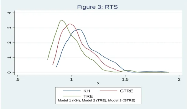
Efficiency estimates in all stochastic frontier models are based on the residuals. Thus, it is important to make sure that the technology is specified properly. If the estimated technology is mis-specified, the resulting residuals will be wrong which in turn is likely to give inappropriate estimates of efficiency scores. Note that the deterministic part of all the three models is specified exactly in the same (all are translog). However, the estimated parameters differ because the error structure in each model is different and their variances through subsequent variable transformation affect the cost function parameters estimates. Since the likelihood ratio tests reject Models 1 and 2, we treat Model 3 as the best model for the data. We report RTS and TC from all three models for a robustness check. Percentile distributions of both RTS and TC from Models 1-3, respectively, are reported in Tables 2-4. Although RTS are calculated from the same translog cost function, their estimates are different for different models. Model 1 gives the highest estimates in almost all percentiles and about 75 per cent of the observations show increasing RTS, the median being 1.08. Model 2 predicts increasing RTS for about half of the data points and the median is 0.95. So the prediction of Model 2 is different from Model 1 for many airlines. Estimates of RTS from Model 3 are in between. The median value of 1.022 is slightly above unitary RTS. A close look at their density plot in Figure 3 shows that the distribution looks alike but is pushed to the right starting from Model 2 to Model 3 to Model 1.

Figure 3. RTS.

TC in a cost function is technical progress if the sign is negative (meaning that ceteris paribus the cost decreased over time). Thus, all three models show technical progress at the mean/median, at the rate

0 1 2 3 4 .5 1 1.5 2 x KH GTRE TRE

Model 1 (KH), Model 2 (TRE), Model 3 (GTRE)

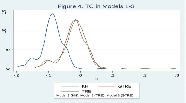
of 1.6 to 1.7 per cent per year in Models 2 and 3, and at a much higher rate of 8.74 per cent in Model 1. However, technical regress (positive value of TC) is also observed for some airlines, and their numbers are model specific. The distribution of TC (reported in Figure 4) shows that Model 1 predicts unbelievably high rates of technical progress for almost all the airlines in every year. This is not the case in Models 2 and 3, which are very similar in all percentiles. Median TC (progress) in Models 2 and 3 is 2.07 per cent per annum.

Figure 4. TC in Models 1-3.

There is no one-to-one relationship between high cost efficiency, technical progress and increasing returns to scale. However, one can expect that a low persistent efficiency level gives an opportunity to engage in activities that can reduce inefficiency through a combination of technical progress and increasing scale economies. A high level of transient efficiency level can be attained not only through technical progress and economies of scale but also through better management and various cost reduction reforms and measures mentioned previously. Improvements in transient efficiency can happen through policies and learning by doing.

6. Summary and Conclusion

This paper estimated cost efficiency of 39 international airlines from 33 countries. The airlines’ cost efficiency was analysed using three state-of-the-art stochastic frontier panel data models. The most flexible model (Model 3) accommodated an error structure that has four components. The model distinguished between firm heterogeneity, time-invariant persistent inefficiency, as well as transient (time-variant) inefficiency and random error components. The other two models are special cases of Model 3. All three models were estimated by the maximum likelihood method using distributional assumptions on the error components. From the estimated persistent and transient efficiency components we computed overall efficiency for each airline and time period.

The flexible cost model used here has an advantage over the traditional frontier panel data models in separating airlines’ heterogeneity and persistent efficiency. The mean and dispersion of cost efficiency amongst airlines differ by model specifications and various airline characteristics. The

0 5 10 15 -.2 -.1 0 .1 .2 .3 x KH GTRE TRE

Model 1 (KH), Model 2 (TRE), Model 3 (GTRE)

performance difference can be attributed to and explained by airline and market characteristics like geographic area of operations, size of the airline, different market structures, deregulation processes, competitive conditions and strategic alliances with competitors.

Efficiency results from the model where airline-specific heterogeneity effects are confounded in persistent inefficiency (Model 1) showed that the model is likely to generate estimates of efficiency that are biased downwards. This results in relatively low mean and large dispersion in the persistent and overall components of efficiency. As expected treating airline-specific effects as firm heterogeneity (Model 2) results in similar levels of transient efficiency and in the absence of capturing persistent efficiency the overall efficiency is biased upwards. The results from these two models suggest that variations in airline-specific persistent efficiency are large reflecting cumulative improvements in transient efficiency through learning by doing over time.

The true efficiency level is somewhere in between those obtained from Models 1 and 2. In order to estimate the level of efficiency that is close to the truth, Model 3 was estimated. This model overcomes the limitations of the previous two models by using a four-component error term that allows us to capture the presence of persistent time-invariant efficiency. The model enables separating and accounting for transient efficiency and firm heterogeneity components. Since the likelihood ratio tests reject Models 1 and 2, we treat Model 3 as the best model for the data. The resulting overall efficiency level is somewhere between the first two models reducing downward and upward biases due to model mis-specification. The model results in persistent efficiency with higher mean and low dispersion as well as lower overall efficiency.

An analysis of the distribution of efficiency confirms significant heterogeneity and dispersion. The results show much variation across airlines and over time in temporal changes in efficiency. This is confirmed by the distribution of the efficiency components. Kernel density plots show that the distribution of the transient components in Models 1 and 2 is almost identical. Most of the airlines are found to have high efficiency. The estimation results based on the generalized Model 3 overcome the limitations of the previous two models. Equality, however, is not the case in Model 3. Although the distribution has a long left tail, its mean is about 10 per cent lower.

We calculated returns to scale and technical change which are defined in the same way in all the three models and reported the results for a robustness check. The Kernel density of technical change and returns to scale specifications in general indicated similar dispersion but different concentrations. A close look at the density plots of returns to scale showed that the distributions look alike but are pushed to the right starting from Model 2 to Model 3 to Model 1. The distribution of technical change shows that Model 1 predicts high rates of technical progress for almost all the airlines in every year. This is not the case in Models 2 and 3, which are very similar in all percentiles.

Acknowledgements

The authors would like to thank two anonymous referees and an editor of the journal for their valuable comments and suggestions that helped to improve a previous version of this paper.

References

Arellano, M., and Bond, S. (1991). Some tests of specification for panel data: Monte Carlo evidence and an application to employment equations. Review of Economic Studies, 58, 277-297.

Assaf, A. G., and George, J. A. (2009). The operational performance of UK airlines: 2002-2007. Journal of

Economic Studies, 38 (1), 5-16.

Assaf, A. G., and Josiassen, A. (2012). European vs. US airlines: performance comparison in a dynamic market. Tourism Management, 33, 317-326.

Baltagi, B.H. (2013). Econometric Analysis of Panel Data. Fifth Edition. Wiley.

Barbot, G., Costa, A., and Sochirca, E. (2008). Airlines performance in the new market context: a comparative productivity and efficiency analysis. Journal of Air Transport Management, 14, 270-274.

Barros, C. P., and Couto, E. (2013). Productivity analysis of European airlines, 2000-2011. Journal of Air

Transport Management, 31, 11-13.

Barros, C. P., Liang, Q. B., and Peypoch, N. (2013). The technical efficiency of US airlines. Transportation

Research Part A: Policy Practice, 50, 139-148.

Barros, C.P. and N. Peypoch (2009). An evaluation of European airlines' operational performance.

International Journal of Production Economics 122, 525-533.

Battese, G. E., and Coelli, T. J. (1988). Prediction of Firm-Level Technical Efficiencies with a Generalized Frontier Production Function and Panel Data. Journal of Econometrics, 38, 387–399.

Battese, G. E., and Coelli, T.J. (1995). A model for technical inefficiency effects in a stochastic frontier production function for panel data. Empirical Economics, 20, 325-332.

Bhadra, D. (2009). Race to the bottom or swimming upstream: performance analysis of US airlines. Journal

of Air Transport Management, 15 (5), 227-235.

Butler, J. S., and Moffitt, R. (1982). A Computationally Efficient Quadrature Procedure for the One Factor Multinomial Probit Model. Econometrica, 50 (3), 761-764.

Capobianco, H. M. P., and Fernandes, E. (2004). Capital structure in the world airline industry.

Transportation Research Part A: Policy and Practice, 38, 421-434.

Chang, Y. T., Park, H. S., Jeong, J. B., and Lee, J. W. (2014). Evaluating economic and environmental efficiency of global airlines: a SBM-DEA approach. Transportation Research Part D: Transport and

Environment, 27, 46-50.

Chen, Y. Y., Schmidt, P., and Wang, H.J. (2014). Consistent estimation of the fixed effects stochastic frontier model. Journal of Econometrics, 181 (2), 65-76.

Chiou, Y. C., and Chen, Y. H. (2006). Route-based performance evaluation of Taiwanese domestic airlines using data envelopment analysis. Transportation Research Part E: Logistics and Transportation Review 42, 116-127.

Choi, K., D. Lee and D.L. Olson (2013). Service quality and productivity in the US airline industry: a service quality-adjusted DEA model. Service Business, 9, 1-24.

Clougherty, J. A., and Zhang, A. (2009). Domestic rivalry and export performance: theory and evidence from international airline markets, Canadian Economics Association. Canadian Journal of Economics, 42 (2), 440-468.

Coelli, T., Perelman, S., and Romano, E. (1999). Accounting for environmental influences in stochastic frontier models: with application to international airlines. Journal of Productivity Analysis, 11, 251-273. Colombi, R., Kumbhakar, S.C., Martini, G., and Vittadini, G. (2014). Closed-skew normality in stochastic frontiers with individual effects and long/short-run efficiency. Journal of Productivity Analysis, 42, 123–136. Cosmas, A., Love, R., Rajiwade, S., and Linz, M. (2013). Market clustering and performance of U.S. OD markets. Journal of Air Transport Management, 28, 20-25.