http://www.diva-portal.org
This is the published version of a paper presented at ECOS 2018 - the 31st International
Conference on Efficiency, Cost, Optimization, Simulation and Environmental Impact of Energy Systems, 17-21 June, 2018, Guimarães.
Citation for the original published paper: Ahlgren, F., Thern, M. (2018)
Auto Machine Learning for predicting Ship Fuel Consumption
In: Proceedings of ECOS 2018 - the 31st International Conference on Efficiency, Cost,
Optimization, Simulation and Environmental Impact of Energy Systems Guimarães
N.B. When citing this work, cite the original published paper.
Permanent link to this version:
PROCEEDINGS OF ECOS 2018 - THE 31ST INTERNATIONAL CONFERENCE ON
EFFICIENCY, COST, OPTIMIZATION, SIMULATION AND ENVIRONMENTAL IMPACT OF ENERGY SYSTEMS
JUNE 17-22, 2018, GUIMARÃES, PORTUGAL
Auto Machine Learning for predicting Ship Fuel
Consumption
Fredrik Ahlgrena, Marcus Thernb
a Linnaeus University, Kalmar Maritime Academy, Sweden, fredrik.ahlgren@lnu.se b Lund University, Lund, Sweden, marcus.thern@energy.lth.se
Abstract:
In recent years, machine learning has evolved in a fast pace as both algorithms and computing power are constantly improving. In this study, a machine learning model for predicting the fuel oil consumption from engine data has been developed for a cruise ship operating in the Baltic Sea. The cruise ship is equipped with legacy volume flow meters and newly installed mass flow meters, as well as an extensive set of logged time series data from the machinery logging system. The model is developed using state-of-the-art Auto Machine Learning tools, which optimises both the model hyper parameters and the model selection by using genetic algorithms. To further increase the model accuracy, a pipeline of different models and pre-processing algorithms is evaluated. An extensive model trained for a certain system can be used for optimisation simulation, as well as online energy efficiency prediction. As the models automatically adapt to noisy sensor data and thus function as a watermark of the machinery system, these algorithms show a potential in predicting ship energy efficiency without installation of additional mass flow meters. All tools used in this study are Open Source tools written in Python and can be applied on board. The study shows great potential for utilising large amounts of already available sensor data for improving the accuracy of the predicted ship energy consumption.
Keywords:
Ships, Auto Machine Learning, Predicting Fuel Consumption, Energy Efficiency.
1. Introduction
An accurate prediction of the fuel consumption of the engines on a ship is important/useful to be able to calculate energy flows, as a basis for energy models, as well as an economic incentive of predicting operational costs. There is often a large amount of measurements already available from the engines which can be used as features for modelling the fuel consumption. This implies that already available engine measurements can be used to train a computer model instead of installing additional mass flow meters. In recent years, machine learning has evolved in a fast pace, as both algorithms and computing power are constantly improving.
One of the challenges in modelling energy systems consist of having accurate predictions of specific parts of the system. The idea for this study was formed during the development of modelling of the energy system of a cruise ship. In two previous studies, an organic Rankine cycle was simulated on the operational load profile [1,2]. In two other studies on the same energy system an analysis of all energy flows was analysed [3,4]. In these studies, the fuel oil (FO) consumption was modelled with a white box approach and then calibrated with a correction factor for each days’ total FO consumption. The problem with this approach is that all engines are treated as a generalized model and does not take into account individual differences. The measured logged data from the on-board logging system, is also of unknown quality.
The framework for machine learning utilised in this study is scikit-learn [5], which is a well-known and often used library for machine learning. It is free of charge, open source and runs on Python (Python Software Foundation, https://www.python.org/), which makes it accessible for a wide range of computing platforms.
Choosing the right machine learning algorithm is often a challenge. With a simple model, such as a linear fit, the model may not be accurate enough. It can also be hard to know which features that should be put in to the training of the model and to tune the hyper parameters. Auto machine learning
(AML) is a concept when the data scientist is replaced by an optimisation algorithm. AML creates black box models which means that the model is trained on the data, regardless of information on how the system works.
Machine learning in shipping has been studied before. Corradu et al. [6] has developed a mixed white and black box model which they call gray-box modelling, in which the black box approach of machine learning is combined with a model based upon physical constraints and equations. The approach of using a combination of white and black box models gives the added advantage of feeding those physical constraints and equations that are known into the training. In a study applying multi-class support vector machines for energy efficient operations [7], a ML-model was developed for predicting a ships’ energy efficiency profile. A ML-model using a neural network for trim optimisation was developed in 2010 for a ferry, using installed on-board sensors for propeller pitch, rudder angle, fuel properties and wind speed and vessel speed etc. [8].
In previous studies on data from the same ship as in the present study [1,9–11] a white box approach was used on the same dataset for predicting the FO consumption. The model was comprised of the fuel rack position and engine rpm, in combination with the fuel characteristics such as density and heating value. The white box model was then calibrated against each days’ FO consumption with a constant. This method demonstrated results within an error margin of 3% [9].
When using optimisation routines, Auto machine learning has proved to be best for both choosing type of ML-algorithm, as well as for tuning of its hyperparameters. Auto-Sklearn uses Bayesian optimisation methods on available scikit-learn algorithms for pre-processing and choosing algorithm and tuning of hyperparameters [12]. Olson et al. has developed an optimisation tool called Tree-based Pipeline Optimisation Tool (TPOT), for automating the previous manual work of pre-processing the data and choosing algorithms [13]. The TPOT tool uses genetic algorithms to optimise both the pre-processing data as well as machine learning algorithm with their respective hyper parameters. It pipelines models which means that they are coupled in series for a maximum model fit.
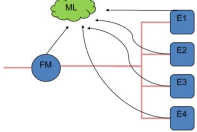
In this study we utilise machine learning to predict the engine’s fuel flow. The engines are modelled as black boxes which means that there are no physical equations used in the model. If the model is fed with an adequate amount of data for training, it will distinguish the individual engines fuel oil consumption, even with only one measured value for training. As presented in Fig. 1, the ML-model needs to have training data from the engines as well as a prediction for the model. During training, one engine might be running on a low load, one other on a higher load, as well as a varying constellation of combinations. This all adds up to a machine learning model which tries to minimise the error? for all scenarios, and thereby it will learn the individual engines characteristics even though it is never measured. It can be argued that this means additional fuel meters are redundant.
This article demonstrates how ML can be used to improve existing models for simulation of energy systems. The work presented in this study can be used as a means to better tune existing models for simulation of energy systems, and to increase accuracy to fuel predictions of data from existing ship logging systems. In order to get correct estimates for energy flows of a ship, the FO consumption is the baseline for all energy input on the ship.
1.1 The cruise ship M/S Birka Stockholm
The study was conducted on the cruise ship M/S Birka Stockholm shown in Fig. 2. The ship is, in a global perspective, a medium sized cruise ship. It is only operating passengers for daily leisure cruises between Stockholm, Sweden and Mariehamn, Åland. The ship is 180 m long and, has a capacity of a total of 1800 passengers.
Fig. 2. The cruise ship M/S Birka Stockholm
The ship leaves every afternoon at 18.00 from Stockholm and slowly cruises thru the archipelago until it reaches the open Åland Sea at around midnight. During the first part in the archipelago the speed is limited both in max and minimum due to navigational restrains. A minimum of two main engines are running due to navigational safety as the ship is more manoeuvrable when running two propellers. During the night it slowly travels, or just drifts along on the sea, until it reaches Mariehamn at the morning around 08.00. It is a very short stop in Mariehamn before the ship goes back to Stockholm. The operational profile is almost identical for each day with some exceptions of longer cruises in the Baltic Sea during the summer.
The energy system for a cruise ship is complex due to the large number of facilities for the passengers’ comfort and entertainment, including several restaurants, shops, night-clubs and spa facilities. The propulsion system consists of four main engines in which are connected via two gearboxes to two outgoing shafts. The propellers are controllable pitch (CPP) propellers, which means that the thrust can be controlled by not only the propeller rpm but also the propeller pitch. The main propulsion system has a total nominal power of 23 400 kW, the engines are four stroke diesel engines Wärtsilä 6L46B, each with a nominal power of 5850 kW. The electricity on board is produced by four diesel generators, called auxiliary engines. The main engines 1 and 3 (ME1 and ME3) and auxiliary engines 1 and 3 (AE1 and AE3) are connected to the starboard fuel meter, and engine pairs 2 and 4 (ME2, ME4, AE2 and AE4) to the port fuel meter. The fuel lines are in this paper named fuel line 1/3 and 2/4.
During the time period for this study, all engines were running on either marine diesel oil (MDO) or a low sulphur heavy fuel oil (HFO). MDO is a more distilled and cleaner fuel compared to HFO, but at an added cost. During the time period for this study all engines expect one auxiliary engine (AE2) were running on heavy fuel oil. Before 1st of January 2015 a maximum amount of 0.5 % sulphur were allowed in the fuel when operating in the Baltic Sea [14]. When running the generator in port it is not allowed to burn HFO by local regulations, and therefore one diesel generator is always connected to marine diesel oil. The diesel oil is not measured by neither of the fuel oil meters used in this study.
2. Method
2.1. Data acquisition
The data from the ship was manually collected by extracting data from the on board Valmarine logging servers using a USB-stick. Totally a period of 14 months’ worth of data was extracted. The meta data from ship logging systems are not standardised and all measured data points needed to be manually treated. The identification of data-points needed to be validated against both the ship schematics and also by talking with the machinery crew. The data is collected from two sources, the Valmarine machinery logging system and the ships logbook.
The Valmarine logging system consists of 2500 data points that are logged in the database with a 1-minute interval. The exported value is an average made by the database export tool of 1-1-minute database sample measurements. The database export tool was based on a legacy Microsoft Excel 2007 plugin, which meant that a maximum of 65 536 rows could be exported each round. The data was exported to Excel-files which then was merged and consolidated into one HDF5-database with the Python library Pandas [15].
The Valmarine machinery logging system logs the temperatures, fuel flows and engine variables in the ship. The FO consumption is mainly measured with volume flow meters that was installed when the ship was built in 2004. There are two FO-meters for a total of eight engines; two main engines and two auxiliary generators per flow meter. The FO-consumptions was logged in the logging system in a 15-minute interval. The measurements collected from the machinery system are not calibrated, and it is also the fact that for instance each time the engine crew changes a fuel pump the readings of the fuel rack position could be at a significant offset if no calibration is made. This implicates that there are uncertainties of the measured data.
In 2014, new mass flow meters were installed with the intention of connecting them to the ship logging system, but during the time of the data collection, these readings were only manually recorded in the engine log book. Thus, this dataset comprises only manually recorded values from the mass flow meters, and as the crew manually recorded this each midnight it implies a large uncertainty of each days’ consumption. As this is a manual routine it can differ quite significant in exact time of day when each reading is done, and that is not logged, only the total for each day. That implies that a reading which was done at 00:30 at day 1, and the next reading at 22:30 day 1 gives a reading in the logbook of mass flow amount -1h day 1, and if consistent an additional +1h flow the next day. Considering an average fuel consumption, even a 30 minute early or late recording can result in about 2 % difference in that days logged consumption. During a longer time span the difference would fade away. The mass flow meters are still considered to be the most accurate measurement, as it has a stated accuracy of 0.5%, and accounts for the density and temperature.
Furthermore, the fuel oil quality is unknown. Depending on supplier and current batch of fuel oil, the calorific heat content, viscosity and density can be different which gives an added uncertainty to the fuel oil consumption. In this way the study started with validation of the legacy installed volume flow meters, comparing each day of operation for mass flow meters and volume flow meters.
2.2. Pre-process
In this section a short analysis of the correlation of each days’ sum is made, as we have readings from both mass flow meters daily sum and dynamic readings from the older volume flow meters. It is possible to overcome the uncertainty of the fuel-flow if it is possible to fit the volume flow meter to the mass flow meter. In that way, it is possible to verify and thus minimize the uncertainty of the mass flow data. This section thus validates the data used for the fuel flow.
The training process depends on the quality of the data. If the model is to be trusted the predictor needs to be validated. The aim of the training is to find a way to predict the fuel flow with different inlet parameters. This means that it is desirable to have as high resolution as possible on the fuel flow data. As the ship is equipped with both volume flow meters and mass flow meters that monitor the
fuel flow where the mass flow meters are the most accurate source of data available. If the machine learning model is trained on the wrong data, it will try to minimise the error on what it is trained with. If the model is to be trusted the predictor needs to be validated. In this dataset the most accurate reading is the daily sum from the mass flow meters, as they are independent on the fuel properties. The volume flow meters do not directly measure the mass flow, which means that the fuel properties such as temperature and density can vastly influence the calculated mass flow. As we did not have dynamic readings of the mass flow meters, the ML-algorithm was trained with 15-min interval data. Therefore, the volume flow meters were validated with data from the mass flow meters.
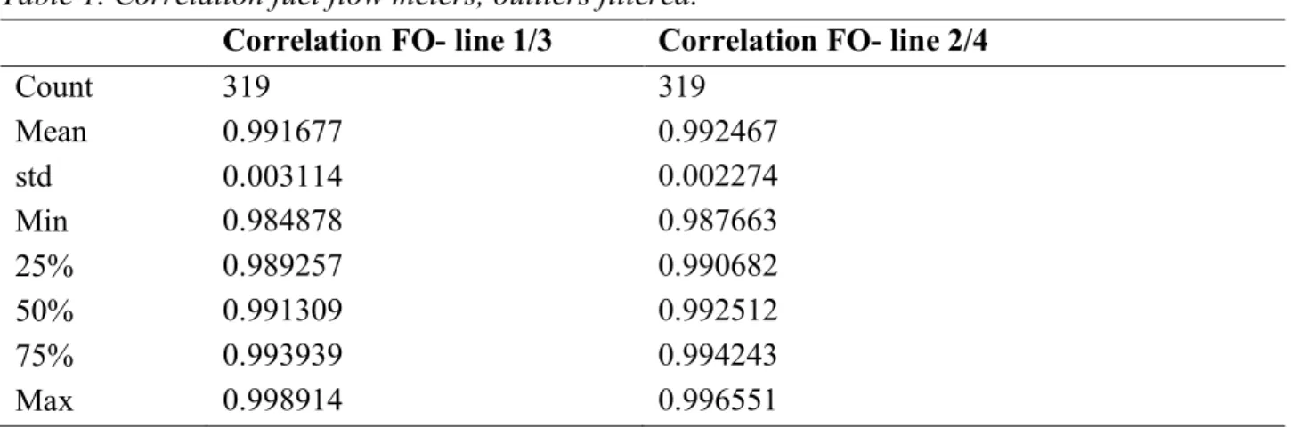
There are no readings from the mass flow meters before 2014-02-01 so that time period is filtered out. All data was filtered for NaN (not a number), and as we assume there is no back blow all values below zero was set to zero. A new dataset was created with the sum for each day volume flow meter. The analysis demonstrated that the correlation between the flow meters were inconsistent in December 2014, this is due to an early fuel shift as the sulphur limit for the Baltic sea emission control area was lowered to 0.1% the 1st January 2015. All logged fuel data of December 2014 was filtered out due to this fact. As presented in Table 1, the correlation between the flow meters are consistent within 0.003113-0.002274 standard deviations if the outliers are filtered out.
Table 1. Correlation fuel flow meters, outliers filtered.
Correlation FO- line 1/3 Correlation FO- line 2/4
Count 319 319 Mean 0.991677 0.992467 std 0.003114 0.002274 Min 0.984878 0.987663 25% 0.989257 0.990682 50% 0.991309 0.992512 75% 0.993939 0.994243 Max 0.998914 0.996551
2.3. Model setup
Supervised learning is the concept of manually choosing the best algorithm for a machine learning task, and this relies much on the experience of the data scientist as well as trying different setups. The ML-algorithms also has a large number of parameters that can be tuned, and some algorithms perform better with a scaling the input data. The concept of Auto Machine Learning (AutoML) is to automate this task, and in this study two AutoML libraries are used.
The AutoML tools used in this study are the Tree Pipeline Optimisation Toiol (TPOT) library and the Auto Sklearn (AutoSk) library [12,13]. These tools optimise the supervised part of the ML-process, programmed to minimise the error for a machine learning pipeline. A ML-pipeline is when combining several ML-algorithms and pre-processors in series. Both tools are utilising the extensive Python Scikit-learn library as the ML-algorithm toolbox [5].
2.4. Model training
Given the fuel flow data it is now possible to train a model for the fuel flow. There are a number of different options of input parameters that can be used as features for the model. M/S Birka Stockholm has the following features available: fuel rack position (frp), exhaust gas temperature (exh_T), engine RPM (rpm) and turbo charger RPM (TC_rpm). These parameters were also chosen because they are
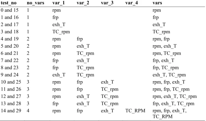
often available in a standard logging engine system setup. It is however not always the case and it is therefore of interest to study what parameters are needed to get a satisfactory result for the fuel flow. Using the features available at M/S Birka it is possible to form a set of different input data. These combinations are given in Table 2. The test setup consists of 30 possible combinations for each model setup, and a total of 90 models for linear, TPOT and AutoSk. The training sets are numbered according to the Python standard, with integers 0-29. As there are two identical fuel lines, tests 0 and 15 are the same, and so on, but on either fuel line. Each of these combinations are trained with a ML, a linear model, and by two AutoML tools, TPOT and auto-sklearn.
Table 2. Test training setup and ML features.
test_no no_vars var_1 var_2 var_3 var_4 vars
0 and 15 1 rpm rpm
1 and 16 1 frp frp
2 and 17 1 exh_T exh_T
3 and 18 1 TC_rpm TC_rpm
4 and 19 2 rpm frp rpm, frp
5 and 20 2 rpm exh_T rpm, exh_T
6 and 21 2 rpm TC_rpm rpm, TC_rpm
7 and 22 2 frp exh_T frp, exh_T
8 and 23 2 frp TC_rpm frp, TC_rpm
9 and 24 2 exh_T TC_rpm exh_T, TC_rpm
10 and 25 3 rpm frp exh_T rpm, frp, exh_T
11 and 26 3 rpm frp TC_rpm rpm, frp, TC_rpm
12 and 27 3 rpm exh_T TC_rpm rpm, exh_T, TC_rpm
13 and 28 3 frp exh_T TC_rpm frp, exh_T, TC_rpm
14 and 29 4 rpm frp exh_T TC_RPM rpm, frp, exh_T, TC_RPM
A total of 90 models were trained by linear regression, TPOT optimisation for 10 generations and auto-sklearn regression. The training was fed in to the fitting function with the corresponding features for each run, and the corresponding measured fuel flow for the FO meter. The classic approach to training a model is by dividing the dataset into two randomised sets, one training set and one test set. Depending on how large the dataset is a somewhere between 80/20 to 50/50 is considered [16], where a larger dataset might have a smaller test set fraction. The dataset was split with the sklearn train test split tool into 75% train data and 25% test data. The random seed for splitting the train and test set was manually set to 42 as to get a reproducibility.
As Sklearn does not utilise the GPU for processing it solely relies on the CPU, and it can utilise all cores. In this setup a server using Ubuntu Linux LTS 16.04 with an Intel Xeon E3-1200 CPU, which has 8 cores and 8 virtual cores. The training took approximately 40 hours. The Anaconda Python 3.6.4 distribution was used, with all packages up to date. TPOT version 0.9.2, Pandas version 0.22.0, Numpy 1.14.0 and Scikit-learn 0.19.1
3. Results and discussion
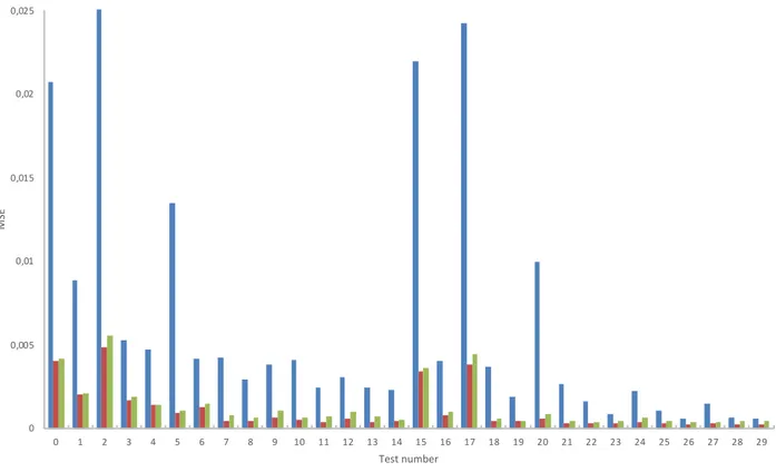
The results demonstrate that the TPOT models are within 0.004833624 standard deviations and auto-sklearn 0.005572236 standard deviations of the measured value in all tests, in comparison with the linear models with 0.025050563. In Fig. 3 it is demonstrated that the linear models show poor performance against the auto-ML methods. Note that the tests 0-14 are identical to 15-29 but on different fuel lines. The model trained on fuel line 2/4 (tests 15-29) demonstrated better performance. All AutoML model perform significantly better than the linear model baseline, which is also what could be expected.
Fig. 3. Mean squared error test results
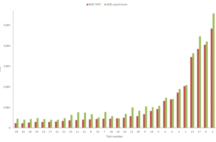
In Fig. 4 the test numbers are sorted on TPOT mean squared error (MSE) from best to worst performance, with a comparison with the auto-sklearn. The TPOT models demonstrated better performance than auto-sklearn.
0 0,005 0,01 0,015 0,02 0,025 0 1 2 3 4 5 6 7 8 9 10 11 12 13 14 15 16 17 18 19 20 21 22 23 24 25 26 27 28 29 MS E Test number MSE Linear MSE TPOT MSE autosk-learn
Fig. 4. Mean squared error, comparison TPOT and autosk-learn
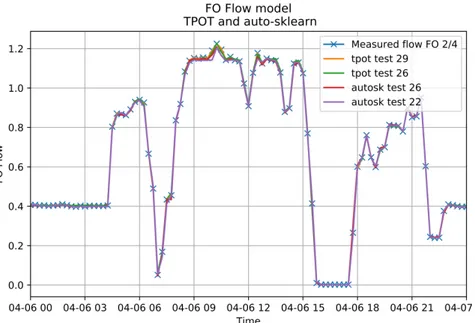
The six best performing tests are plotted in Fig. 5 as the difference between the model estimate and the measured value during an arbitrary day (2014-04-06 00:00 to 2014-04-07 00:00), it can be seen that there are some larger deviations of the model predictions at 15:00 and at 18:00. This is when the ship is manoeuvring in port, which means a lot of manoeuvring and as the data input for the model are averaged in 15-min interval dynamics from shorter time intervals are missed. As shown in Fig. 6, where only the TPOT and auto-sklearn models are shown, the model test TPOT 29 stands out.
Fig. 5. Best performing models, showing model difference
0 0,001 0,002 0,003 0,004 0,005 29 26 28 25 23 27 22 21 24 11 13 8 14 7 18 19 10 12 20 9 16 5 6 4 3 1 15 17 0 2 MS E Test number MSE TPOT MSE autosk-learn
As shown in Fig. 6 the TPOT test 29 is only off by approximately 0.027 m3/h at the 2014-04-06 18:00, in relative terms that is a deviation of less than 4.5% at one single point.
Fig. 6. Best model performance TPOT and auto-sklearn.
Fig. 7. TPOT and auto-sklearn models compared to measured flow.
In Fig. 7 the fuel consumption of fuel line 2/4 is shown in absolute terms during the same time period, plotted with the model value over the measured value.
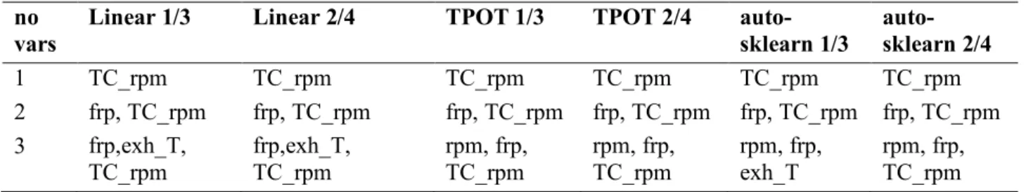
3.1 Feature ranking
In Table 3 the engine training features are sorted for the lowest MSE, and it shows that if only using one engine feature the turbocharger RPM is the best model performing feature. When using two features, the engine fuel rack position provides the best addition. Both one and two variables show consistency in ranking between all tests, but when training with three features the linear model gives best performance with the addition of the exhaust gas temperature. The TPOT model for both fuel lines and the auto-sklearn 2/4 give better results with the addition of the engine rpm. It is only the auto-sklearn model for the fuel line 1/3 which stands out in the AutoML models in the three-variable ranking.
Table 3. Features for best ranked MSE.
no vars
Linear 1/3 Linear 2/4 TPOT 1/3 TPOT 2/4 auto-sklearn 1/3 auto-sklearn 2/4 1 TC_rpm TC_rpm TC_rpm TC_rpm TC_rpm TC_rpm 2 frp, TC_rpm frp, TC_rpm frp, TC_rpm frp, TC_rpm frp, TC_rpm frp, TC_rpm 3 frp,exh_T, TC_rpm frp,exh_T, TC_rpm rpm, frp, TC_rpm rpm, frp, TC_rpm rpm, frp, exh_T rpm, frp, TC_rpm
4. Conclusion
The AutoML methods has demonstrated a large advantage over a standard linear regression training, and by only using a few features from the engines it is still possible to train a model which predicts consistently within a very small margin. By using AutoML methods, the time needed for manually evaluating and trying different machine learning algorithms is by far reduced and will also provide a very accurate model.
The AutoML models used in this study are open source and freely available to use as a concise and straight forward method for further refining the baseline for other black box ML-models, or real-world predictions. The models can estimate the performance of each engine without installing flow meters for each individual engine. It is also possible given enough data, to use data of a lower interval such as daily or weekly bunker data, to train a model on engine features in which are recorded with a higher interval to make dynamic predictions.
Acknowledgments
The authors wish to give acknowledgment to the Swedish Maritime Administration, Linnaeus University and Lund University for their financial support. We also acknowledge Eckerörederiet and the engine crew of M/S Birka Stockholm for their support and access to ship data.
References
[1] Mondejar ME, Ahlgren F, Thern M, Genrup M. Quasi-steady state simulation of an organic Rankine cycle for waste heat recovery in a passenger vessel. Appl Energy 2017;185. doi:10.1016/j.apenergy.2016.03.024.
[2] Ahlgren F, Mondejar ME, Genrup M, Thern M. Waste Heat Recovery in a Cruise Vessel in the Baltic Sea by Using an Organic Rankine Cycle: A Case Study. J Eng Gas Turbines Power 2015;138:011702. doi:10.1115/1.4031145.
[3] Baldi F, Ahlgren F, Nguyen T-V, Gabrielii C, Andersson K. Energy and exergy analysis of a cruise ship. ECOS 2015 - 28th Int. Conf. Effic. Cost Optim. Simul. Environ. Impact Energy Syst., 2015.
[4] Baldi F, Ahlgren F, Melino F, Gabrielii C, Andersson K. Optimal load allocation of complex ship power plants. Energy Convers Manag 2016;124:344–56. doi:10.1016/j.enconman.2016.07.009.
[5] Pedregosa F, Varoquaux G, Gramfort A, Michel V, Thirion B, Grisel O, et al. Scikit-learn: Machine Learning in Python 2012;12:2825–30. doi:10.1007/s13398-014-0173-7.2.
[6] Coraddu A, Oneto L, Baldi F, Anguita D. Vessels fuel consumption forecast and trim optimisation: A data analytics perspective. Ocean Eng 2017;130:351–70. doi:10.1016/j.oceaneng.2016.11.058.
[7] Pagoropoulos A, Møller AH, McAloone TC. Applying Multi-Class Support Vector Machines for performance assessment of shipping operations: The case of tanker vessels. Ocean Eng 2017;140:1–6. doi:10.1016/j.oceaneng.2017.05.001.
[8] Petersen JP, Winther O, Jacobsen DJ. A machine-learning approach to predict main energy consumption under realistic operational conditions. Ship Technol Res 2012;59:64–72. doi:10.1179/str.2012.59.1.007.
[9] Baldi F, Ahlgren F, Nguyen T-V, Gabrielii C, Andersson K. Energy and exergy analysis of a cruise ship. ECOS 2015, 2015. doi:10.4236/epe.2012.45047.
[10] Ahlgren F, Mondejar ME, Genrup M, Thern M. Waste heat recovery in a cruise vessel in the Baltic Sea by using an organic Rankine cycle: A case study. J Eng Gas Turbines Power 2016;138. doi:10.1115/1.4031145.
[11] Mondejar ME, Ahlgren F, Thern M, Genrup M. Study of the On-route Operation of a Waste Heat Recovery System in a Passenger Vessel. Energy Procedia 2015;75:1646–53. doi:10.1016/j.egypro.2015.07.400.
[12] Feurer M, Klein A, Eggensperger K, Springenberg J, Blum M, Hutter F. Efficient and Robust Automated Machine Learning. Adv Neural Inf Process Syst 28 2015:2944–52.
[13] Olson RS, Urbanowicz RJ, Moore JH, Bartley N. Evaluation of a Tree-based Pipeline Optimization Tool for Automating Data Science. Proc. Genet. Evol. Comput. Conf. 2016, Denver, Colorado, USA: ACM; 2016, p. 485–92. doi:10.1145/2908812.2908918.
[14] IMO - 2010 - RESOLUTION MEPC.176(58) (Revised MARPOL Annex VI). International Maritime Organization; 2010.
[15] McKinney W. pandas: a Foundational Python Library for Data Analysis and Statistics. Python High Perform Sci Comput 2011:1–9.