A Multi-Level Routing Scheme and Router Architecture
to support Hierarchical Routing in Large Network on
Chip Platforms
Rickard Holsmark1, Shashi Kumar1 and Maurizio Palesi2 1 School of Engineering, Jönköping University, Sweden
{rickard.holsmark, shashi.kumar}@jth.hj.se
2 DIIT, University of Catania, Italy
mpalesi@diit.unict.it
Abstract. The concept of hierarchical networks is useful for designing a large
heterogeneous NoC by reusing predesigned small NoCs as subnets. It can also be helpful when analyzing and designing a large NoC as interconnection of subnets at a higher level of abstraction. Hierarchical deadlock-free routing is required to enable deadlock-free interconnection of sub-networks with different internal routing algorithms. In this paper we show that multi-level addressing is a cost-effective implementation option for hierarchical deadlock-free routing. We propose a two-level routing scheme, which is not only efficient, but also enables co-existence of algorithmic and table-based implementation in one router. A hierarchical view of the network simplifies addressing of network nodes and address decoding in the router. Synthesis results show that a 2-level hierarchical router design for an 8x8 NoC, can reduce area and power requirements by up to ~20%, as compared to a router for the flat network. This work also proposes a new possibility for increasing the number of nodes available for subnet-to-subnet interfaces, while keeping the properties of hierarchical deadlock-freedom. We evaluate and discuss the communication performance in a 2-level hierarchical network for various subnet interface set-ups and traffic situations. A cycle accurate simulator has been developed and used for this purpose.
Keywords: Networks on Chip, Hierarchical Networks, Deadlock Free Routing,
Router Architecture
1
Introduction
While SoCs consisting of tens of cores were common in the last decade, ITRS predicts that the next generation of many-cores SoC will contain hundreds of cores. Intel has recently announced the fabrication of a 48-core chip [1] using a Network-on-Chip as communication infrastructure. The concept of hierarchy will be very useful in
designing and using such NoC platforms with growing number of cores. This concept will allow raising the level of abstraction of reuse during the design process. Instead of reusing IP cores, one can redesign large NoCs by integrating predesigned smaller NoCs as building blocks.
Whether hierarchical or not, the formation of packet deadlocks may be fatal to any network communication. To avoid this, several deadlock-free routing schemes have been proposed in literature, e.g. Turn model [2], Odd-Even [3] and Up*/Down* [4]. Deadlock freedom may be compromised when combining different networks, each with its own deadlock-free routing algorithm. For this reason, an important new issue in hierarchical NoCs is the design of deadlock-free routing algorithms. Holsmark et al. [5] proposed the concept of hierarchical deadlock-free routing and showed that if subnets are interconnected by “safe boundary” nodes, it is possible to design a deadlock-free global routing algorithm without altering any internal subnet routing algorithm. Although design and analysis of the routing algorithm was hierarchical, Holsmark et al. [5] assumed a flat implementation with a common address space for all network nodes. Non-homogeneity in such cases will often require the use of routing tables to implement the routing function.
In this work we propose that a hierarchical routing function is implemented in two levels. The higher level routing function will determine if the destination for a packet is inside or outside the local subnet. If the destination is outside the subnet, the packet is guided to a node at the boundary of the local subnet. From here the external routing function guides the packet (possibly through intermediate subnets) to a boundary node of the destination subnet. If the destination is within the subnet, the lower level routing function itself guides the packet to the destination node. The proposed structured router architecture enables significant reduction in area and power consumption. One important parameter which affects performance is the number of safe boundary nodes of a subnet. Since some routing algorithms provide very few safe nodes, we propose the concept of “safe channels” to attain higher connectivity. The performance of hierarchical routing is compared with common deadlock-free routing algorithms and the effect of varying the number of boundary nodes is explored.
Recently the topic of hierarchical NoCs has caught the attention of researchers. Several aspects have been studied, for example Bourduas et al. [6] have proposed a hybrid ring/mesh interconnect topology to remove limitations of lengthy diameter of large mesh topology networks. In [7], a hybrid mesh-ring NoC topology is proposed which is suitable for future 3-D ICs. A hierarchical on-chip approach is also taken in HiNoC [8], which offers both packet- and stream-based communication services. In HiNoC, the network has two levels of hierarchy; the asynchronously communicating mesh at the top level and an optional synchronously operating fat-tree structure attached to a mesh router network node. Deadlock-free routing in irregular networks often implies a strongly limited set of routing paths. To increase the available paths, Lysne et al. [9] developed a routing scheme, which avoids deadlock by assigning traffic into different layers of virtual channels.
2
Hierarchical Deadlock-Free Routing Algorithms
The methodology for hierarchical routing algorithms [5] enables deadlock-free interaction of independent subnet routing algorithms in hierarchical networks
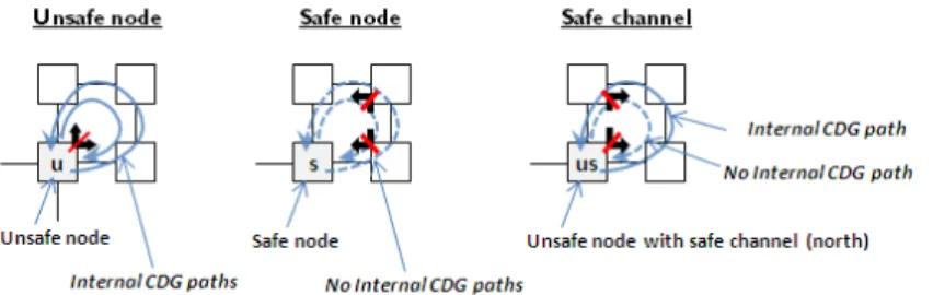
(sub-networks interconnected by external links). Deadlock freedom is guaranteed by acyclic channel dependency graphs (CDG) [10] [11]. In [5] it is shown that if all subnets are deadlock free and all nodes which interconnect subnets are “safe”, it is possible to design a deadlock-free routing algorithm for the whole network. Whether a boundary node is “safe” or not depends on the internal subnet routing algorithm and is easily checked by analysis of internal CDG paths. If there are no paths from any internal output to any internal input of a node, it is safe (see Fig. 1). If such a path exists, the node is unsafe and may enable formation of CDG cycles with paths in other subnets. The concept of safe boundary nodes helps to design a hierarchical routing algorithm by only considering the CDG paths among boundary nodes.
2.1 Safe Channels for Increasing Connectivity
The requirement that all boundary nodes should be safe often, depending on routing algorithm, reduces the number of possible boundary nodes in a network. For deterministic routing algorithms, like XY all nodes are safe boundary nodes. Several partially adaptive algorithms provide few safe boundary nodes, e.g. an NxN network with Odd-Even [3], or West-First [2] provides only N safe boundary nodes. Negative-First [2] would in this case provide N+ (N-1) safe nodes.
To remedy this situation we propose the concept of safe channels. Given a node n, and an internal output channel c of node n, c is a safe channel if there does not exist an internal CDG path from channel c to any input channel of n. Fig. 1 illustrates the differences between unsafe nodes, safe nodes and safe channels.
Fig. 1. Examples of unsafe boundary nodes, safe boundary nodes and safe channels In the safe channel example, it is straightforward to see that only one of the internal output channels of node us (unsafe with safe channel) is on a CDG path to an input channel of us itself. Using this safe channel and restricting the use of the other channel would, from a deadlock-free perspective, be the same as using a safe boundary node. Note that safe channels cannot relax the requirement that there must be at least one safe boundary node in each neighboring subnet. The effect of adding unsafe nodes with safe channels is explored in the evaluation section.
3
Two-Level Routing Scheme
3.1 Addressing and Routing Protocol
Intuitively it seems that the destination address for a packet in a two-level NoC can be encoded using only two fields given in the form: [subnet id, node id]. However the
availability of multiple boundary nodes requires that information of the destination subnet boundary node is added. Therefore a source node tags the header destination address with three fields [subnet id, boundary node, node id].
The routing protocol is identical for all nodes. Each node first checks whether a packet is destined to its own subnet or to an external subnet. If the destination is internal to the subnet, the packet is forwarded using the internal routing function. If the destination is in another subnet, the packet is forwarded by an external routing function (which provides paths identical to the internal routing protocols for internal link traversals).
If subnets are heterogeneous, the encoding of node address in the source subnet may differ from the encoding in the destination subnet, both with respect to size and topology. In general, the header field for node address must be adjusted according to the subnet requiring largest number of bits for node address. The size of the field for subnet addressing depends on the number of subnets.
3.2 Routing Function
The two-level routing function is partitioned into an external routing function RG and
a subnet internal routing function Ri. The internal routing function is identical to the
routing function should the subnet be a stand-alone network. One feature which is enabled by two-level routing is the possibility to utilize different implementation techniques of the internal routing functions in different subnets. This implies that routers in some subnets may be table-based while other routers may implement algorithmic routing.
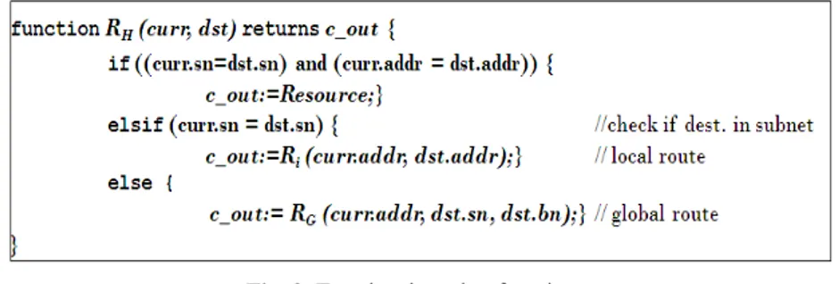
Fig. 2. Two-level routing function
Fig. 2 gives pseudo-code of the main hierarchical routing function RH. The routing
function takes dst which contains the destination subnet (dst.sn), destination boundary node (dst.bn) and node address (dst.addr). If both destination subnet and node address matches with current subnet and node address, the channel will be set to the local resource. Otherwise if the destination resides in the same subnet as the current node, the local routing function is called with the destination node address (dst.addr). The output channel (c_out) will in this case always be internal. Should the subnets not match, the external routing function is invoked with destination subnet (dst.sn) and boundary node (dst.bn). The external routing function can return both external and internal channels if current node is a boundary node. If current node is not a boundary node it will only return internal channels.
The two-level router tables are built using a similar algorithm (breadth first search) as was used for constructing flat router tables. The main difference is that only
paths to destination subnets and boundary nodes are stored in the external table. This means that during the search, for each source-destination pair, the node where the last transition between different subnets was made, is stored as boundary node for the destination. This information is used for addressing by the source node. Simultaneously, the output channel from which the boundary node can be reached is stored in the router table.
Since all paths are obtained using the hierarchical deadlock-free routing methodology [5], it can be shown that the two-level scheme is deadlock free and connected as well. If the destination is in another subnet, such paths must traverse a boundary node in the source subnet and a boundary node in the destination subnet (and possibly also through some intermediate subnets).
3.3 A Small Example of Routing in Two-Level Router Networks
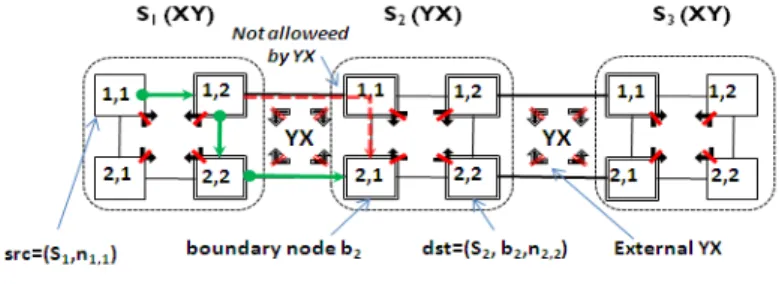
The following simplistic example illustrates routing in two-level networks as well as the necessity for addition of boundary node id for specifying the destination address. Consider Fig. 3 where each of the subnets S1, S2 and S3 is a 2x2 mesh with routing algorithms XY, YX and XY respectively. The external algorithm in this case is assumed to be YX, which is the same as subnet S2 algorithm. Nodes within subnets are addressed using (row#, column#) as shown in the figure. Boundary nodes are indicated by double border.
Fig. 3. Example of two-level addressing
Consider routing a message from source node n1,1 in subnet S1 to the destination node
n2,2 in subnet S2. In two-level addressing, the source node is identified with subnet and node address, src= (S1, n1,1). The source appends the destination address with destination subnet, boundary node and node address, dst= (S2, b2, n2,2). When the routing function is called in curr=src, the subnet fields do not match and the external function will be used. The external function returns the East channel, i.e. RG((n1,1 ), S2, b2) = East. Note that this is the only allowed route according to the internal XY algorithm. At node curr=(S1, n1,2), the external algorithm returns South. Note that East would also not violate the internal algorithm restriction.
However, this shows the necessity for boundary node specification. If the external address is specified using subnet id alone, it would be impossible to distinguish between destinations in row 1 and row 2 in subnet S2. In this case, for reaching node
dst the only allowed route is South, since the packet cannot make this turn at row 1 in
subnet S2 since both the internal algorithm and external algorithm is YX. After turning south, eventually the packet arrives at node n2,1 in subnet S2. Since the current
subnet is now the same as the destination subnet, the node address and local algorithm is used for routing to the destination, i.e. Ri = YX(n2,1, n2,2) = East.
4
Router Architecture with Two-Level Routing Function
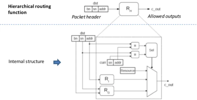
A block diagram of the two-level routing function in the router is given in Fig. 4. As shown in the upper part of the figure, the routing function takes destination subnet address (sn), destination boundary node address (bn), destination node address (addr), and returns the allowed output channel(s) (c_out).
Fig. 4. Internal structure of two-level routing function
Studying the internal structure, it is seen that if both destination subnet and node addresses match with the current subnet and node addresses, the comparators will set the output of the multiplexor to Resource. If the subnet addresses match but not the node addresses, the destination is internal to the subnet and the output from the internal function Ri will be selected. If subnet addresses do not match, the output of
the external function RG will be selected, and the node address is not used. The table
in Fig. 5 presents synthesis results from a 65nm technology library, assuming 1 GHz clock frequency. Network size is set to 64 nodes (8x8 mesh), which is considered as a two-level hierarchical network consisting of four equally sized subnets (4x4 mesh).
The results for implementation of a flat routing function are indicated by the label
RF. Two level routing functions are synthesized for 1, 4 and 7 boundary nodes (RH-1bn, RH-4bn and RH-7bn). The table also provides data for two-level routing with
one boundary node and algorithmic XY routing (RH-1bn-xy). Results are given for one routing function per router. The table gives area and power consumption separately for the routing function as well as the whole router. The main share of cost of the complete router is dominated by input buffers of 4 flits each.
Fig. 5 also summarizes the percentage of area and power reduction of the two level routing functions as compared to the flat routing function. The largest reduction for area, about 65 percent for the routing function (and ~12 percent for the complete router), is obtained by the configuration with one boundary node (bn1), which only needs to store one entry per subnet. As the number of boundary nodes increase so do the resource requirements of the routing function. Power reduction is slightly less than area reduction for all configurations. Considering the algorithmic implementation
Packet header Allowed outputs
Internal structure Hierarchical routing function
with XY as local routing function, it is shown that it is possible to reduce the required area and power for the routing function by about 90 percent.
Fig. 5. Area and power for different two-level router versions(RH-xbn) and a flat router (RF)
5
Performance Evaluations and Results
The evaluations compare performance of hierarchical routing with a few flat routing algorithms (XY, Up*/Down* [4]) with different configurations of boundary nodes and traffic scenarios.
5.1 Evaluation Parameters
The simulator is designed in SDL (Specification and Description Language) using Telelogic SDL and TTCN Suite 6.2 (now IBM Rational). Wormhole switching is employed, with packet size fixed at 10 flits. Routers are modeled with input buffers of size 4 and flit latency of 3 cycles per router. Packet injection rate pir is given in average number of packets generated per cycle. Thus pir=0.02 corresponds to that each node generates on average 2 packets per 100 cycles (Poisson process). For two-level routing, the simulator implements the two-two-level routing protocol described in Section 3, with algorithmically modeled internal subnet routing functions.
Simulations are performed with different levels of external subnet traffic w.r.t. local subnet traffic. This means that for 75% local traffic, 25% of the traffic is sent outside the source subnet. External traffic destinations are uniformly distributed over the whole network. The used subnet configurations are given in Fig. 6(left). Each subnet exhibits a specific traffic type, which in the case of hierarchical routing is matched with a suitable routing algorithm (Subnet 1: Uniformly random, XY; Subnet 2: Transpose1, Negative-First; Subnet 3: Shuffle, East-First (mirrored West-First); Subnet 4: Bit Reversal, Odd-Even).
Fig. 6(right) illustrates the three configurations of boundary nodes and external routing restrictions used in the evaluations. Nodes labeled 1, and links connecting these nodes, are used in the case with one boundary node per subnet (bn1). The set-up with 4 boundary nodes per subnet (bn4) additionally uses the nodes labeled 4 and attached links. The case with 7 boundary nodes per subnet (bn7) uses, in addition to
Synthesis Results
Router Description Routing Function Complete Router Area Power (uW) Area Power (uW) RF Flat 8x8 mesh 3928 2993,4 21781,5 19884 RH-1bn 2L table 1 bn 1268,2 1176,1 19121,6 18066,7 RH-4bn 2L table 4bn 1974,4 1749,1 19827,8 18639,6 RH-7bn 2L table 7 bn 2675,2 2306,2 20528,6 19196,8 RH-1bn-xy 2L tbl/alg 1 bn 317,1 332,7 17569 16426,7 0% 10% 20% 30% 40% 50% 60% 70% 80% 90% 100% RH-1bn RH-4bn RH-7bn RH-1bn-xy Area Power Area and power reduction (routing function) for 2level routers w.r.t. flat router
nodes labeled 1 and 4, the nodes labeled 7. The bn1 and bn4 set-ups utilize only safe nodes, where bn4 represents the maximum attainable connectivity with safe nodes.
Fig. 6. Subnet and boundary node configurations
The bn7 case allows safe channels of unsafe nodes in subnets 3 and 4 and, in this case, achieves the maximum connectivity of the topology. For flat algorithms, the same algorithm is used for all subnets. That is, in the case of XY this means that XY is used for routing over the whole network. Note that XY is only applicable to the bn7 configuration. The Up*/Down* algorithm is applicable to all different configurations and a particular configuration is annotated similarly to the hierarchical (hr_bnx) cases, i.e. ud_bnx. The latency of a packet is the duration from when the packet was generated at the source to when its tail flit was received at the destination. Average latency is the average of all packet latencies in a simulation.
5.2 Comparison of Routing Algorithms and Boundary Node Configurations
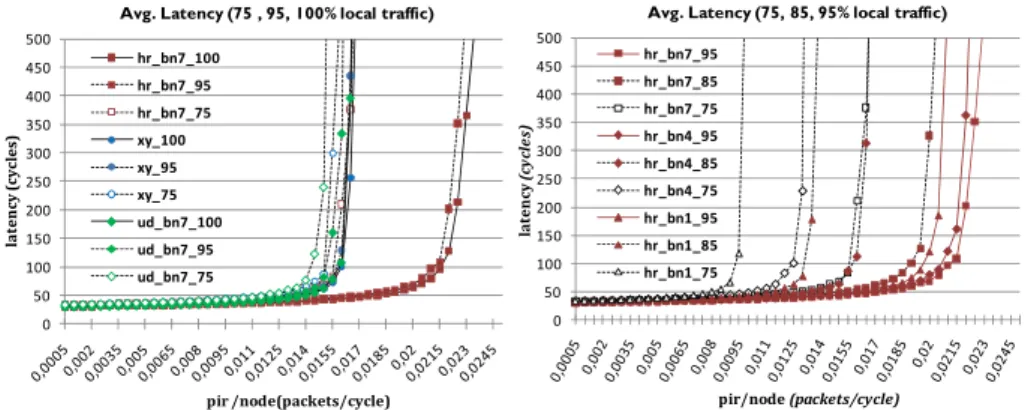
Fig. 7(left) compares average latency of the hierarchical hr_bn7 configuration with XY and Up*/Down* for 100, 95and 75 percent of message subnet locality.
Fig. 7. Average latency: hr vs. other algorithms (left), different hr configurations (right) As can be seen, the performance is adversely affected for all algorithms when reducing the level of internal traffic. The highest performance is, not surprisingly, obtained by hr_bn7 with 100% local traffic (hr_bn7_100). One observation which is
1 1 1 1 1 1 1 1 1 1 1 1 1 1 1 1 1 1 1 1 1 1 1 1 1 1 1 1 1 1 1 1 1 1 1 1 1 1 1 1 1 1 1 1 1 1 1 1 1 1 1 1 1 1 1 1 1 1 1 1 1 1 1 1
Routing algorithms and traffic in subnets Subnet 1 X‐Y Uniform Subnet 2 Neg. First Transpose 1 Subnet 4 Odd Even Bit reversal Subnet 4 East First Shuffle Internal restriction
Boundary node configurations 1 1 1 1 1 1 1 1 1 1 1 1 1 1 1 1 1 1 1 s 1 1 1 1 1 1 1 1 1 1 1 1 1 1 1 1 1 1 1 1 1 1 1 1 1 1 1 1 1 1 1 1 1 1 1 1 1 1 1 1 1 1 1 1 1 bn1 4 4 4 1 4 4 4 4 4 4 4 4 4 7 7 7 7 1 7 7 7 7 7 7 7 7 4 bn4 7 bn7 External restriction 1 4 1 0 50 100 150 200 250 300 350 400 450 500 la te n cy (c yc le s) pir /node(packets/cycle) Avg. Latency (75 , 95, 100% local traffic)
hr_bn7_100 hr_bn7_95 hr_bn7_75 xy_100 xy_95 xy_75 ud_bn7_100 ud_bn7_95 ud_bn7_75 0 50 100 150 200 250 300 350 400 450 500 lat en cy (c yc le s) pir/node (packets/cycle) Avg. Latency (75, 85, 95% local traffic) hr_bn7_95 hr_bn7_85 hr_bn7_75 hr_bn4_95 hr_bn4_85 hr_bn4_75 hr_bn1_95 hr_bn1_85 hr_bn1_75
rather unexpected can be noted. This is seen for hr_bn7 with 95 % local traffic (hr_bn7_95), which performs considerably better than both XY and Up*/Down* with 100% local traffic. For 75% of local traffic, the differences in performance are reduced, especially compared to XY. This is quite expected, since XY is known to be a very good algorithm for uniformly distributed traffic (which is the distribution of the external traffic).
When comparing the results in Fig. 7(left) with hierarchical routing for different configurations of boundary nodes in Fig. 7(right), it is notable that both the four- and one- boundary node hierarchical (hr_bn4_95 and hr_bn1_95 respectively) outperform XY for 95% local traffic, even though the average distances are higher due to the necessity of longer external routes. However, as the local traffic is reduced to 75% and 85%, for hr_bn4 and hr_bn1 respectively, the lesser connectivity of fewer boundary nodes result in notably higher average latency than XY. The very few external links in hr_bn1 are effective bottlenecks and the congestion on these links propagates into the internal subnet traffic.
5.3 Comparison of Effects on Local and External Traffic
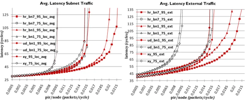
Fig. 8.(left) compares average latency for different algorithms and internal subnet traffic. Both hr_bn7 and hr_bn1 show considerably lower latency values for high load in the 95% local traffic scenario.
Fig. 8. Average latency for internal subnet traffic (left), external traffic (right) Note that XY in this case follows a higher curve than Up*/Down* (ud_bn1_95) at low pir but improves as pir is increased. This indicates that Up*/Down* may have advantage of adaptive routes at lower pir compared to XY routing algorithm. Fig. 8(right) complement the subnet latency by showing the latency of the external traffic. The higher base latency for ud_bn1and hr_bn1, due to less number of external links is visible at both 75% and 95% of local traffic. Still, even though the base latency of
xy_95 is lower, it rapidly increases above the latency of hr_bn1_95 at pir of 0.015.
6
Conclusions
In this paper we have proposed both a new routing scheme as well as a structured router design to support deadlock-free routing in a two-level hierarchical NoC. One
25 45 65 85 105 125 lat en cy (c yc le s) pir/node (packets/cycle) Avg. Latency Subnet Traffic
hr_bn7_95_loc_avg hr_bn7_75_loc_avg hr_bn1_95_loc_avg hr_bn1_75_loc_avg ud_bn1_95_loc_avg ud_bn1_75_loc_avg xy_95_loc_avg xy_75_loc_avg 35 45 55 65 75 85 95 105 115 125 135 la tenc y (c yc le s) pir/node (packets/cycle) Avg. Latency External Traffic hr_bn7_95_ext hr_bn7_75_ext hr_bn1_95_ext hr_bn1_75_ext ud_bn1_95_ext ud_bn1_75_ext xy_95_ext xy_75_ext
important hierarchical network parameter is the number of safe interconnection nodes. We have compared the area and energy consumption of a router for two-level hierarchical networks for various values of this parameter. It is noticed that two-level routing is less costly as compared to a flat solution, especially when only considering the routing function. The importance of this advantage will increase with network size (due to larger tables), if buffer size is kept constant.
We have also evaluated the effect of the number of boundary nodes on communication performance. We observe that two-level hierarchical routing with maximum number of boundary nodes, in general, provides higher performance compared to flat routing algorithms. The advantage is higher when the ratio of external to local traffic is higher. For low external traffic, a single boundary node in each subnet enables routing performance comparable to flat algorithms on fully connected mesh. Multi-level routing embodies a multitude of exploration activities. For example, although the proposed 2-level scheme recursively extends itself to n-levels, implementation issues of such schemes will open new challenges.
References
1. Dighe, S., Hoskote, Y., Vangal, S., Finan, D., Ruhl, G., Jenkins, D., Wilson, H., Borkar, N., Schrom, G., Pailet, F., Jain, S., Jacob, T., Yada, S., Marella, S., Salihundam, P., Erraguntla, V., Konow, M., Riepen, M., Droege, G., Lindemann, J., Gries, M., Apel, T., Henriss, K., Lund-larsen, T., Steibl, S., Borkar, S., De, V., Wijngaart, R.V.D., Mattson, T., Howard, J.: A 48-Core IA-32 Message-Passing Processor with DVFS in 45nm CMOS. International SolidState Circuits Conference. 9, 58-59 (2010).
2. Glass, C., Ni, L.: The Turn Model for Adaptive Routing. Computer Architecture, 1992. Proceedings., The 19th Annual International Symposium on. pp. 278-287 (1992).
3. Ge-Ming Chiu: The odd-even turn model for adaptive routing. Parallel and Distributed Systems, IEEE Transactions on. 11, 729-738 (2000).
4. Schroeder, M., Birrell, A., Burrows, M., Murray, H., Needham, R., Rodeheffer, T., Satterthwaite, E., Thacker, C.: Autonet: a high-speed, self-configuring local area network using point-to-point links. Selected Areas in Communications, IEEE Journal on. 9, 1318-1335 (1991).
5. Holsmark, R., Kumar, S., Palesi, M., Mejia, A.: HiRA: A methodology for deadlock free routing in hierarchical networks on chip. Networks-on-Chip, 2009. NoCS 2009. 3rd ACM/IEEE International Symposium on. pp. 2–11IEEE Computer Society (2009). 6. Bourduas, S., Zilic, Z.: A Hybrid Ring/Mesh Interconnect for Network-on-Chip Using
Hierarchical Rings for Global Routing. Proc. of the ACM/IEEE Int. Symp. on Networks-on-Chip (NOCS). (2007).
7. Rantala, V., Lehtonen, T., Liljeberg, P., Plosila, J.: Hybrid NoC with Traffic Monitoring and Adaptive Routing for Future 3D Integrated Chips. Digest of the Workshop on Diagnostic Services in Network-on-Chips. (2008).
8. Hollstein, T., Ludewig, R., Zimmer, H., Mager, C., Hohenstern, S., Glesner, M.: Hinoc: A Hierarchical Generic Approach for on-Chip Communication, Testing and Debugging of SoCs. VLSI-SOC: From Systems to Chips. pp. 39-54 (2006).
9. Lysne, O., Skeie, T., Reinemo, S., Theiss, I.: Layered Routing in Irregular Networks. IEEE Trans. Parallel Distrib. Syst. 17, 51-65 (2006).
10. Dally, W., Seitz, C.: Deadlock-Free Message Routing in Multiprocessor Interconnection Networks. Computers, IEEE Transactions on. C-36, 547-553 (1987).
11. Duato, J.: A new theory of deadlock-free adaptive routing in wormhole networks. Parallel and Distributed Systems, IEEE Transactions on. 4, 1320-1331 (1993).