Development of a Nordic BWR plant model in APROS and design of a power controller using the control rods

(1)

(2)

Westinghouse Electric Sweden AB

Development of a Nordic BWR plant model in

APROS and design of a power controller using

the control rods

Jonathan Al-Ani

Supervisor at Westinghouse: David Mauritzson

Supervisor at KTH: Sean Roshan Ghias

(3)

i

Abstract

Nuclear power plants have proved to produce reliable and economic electricity but at the same time provoked debates mainly because of the risks involved during operation. To prevent unwanted events, it is important to identify and estimate their occurrence, and introduce measures to counteract them. Modelling and simulations are powerful tools that can be used to gain this type of knowledge and obtain information about the birthplace of incidents. However, the area of use is not limited to the safety perspective, as computer simulations can also introduce true advances in performance and reliability of power plants.

This master thesis was conducted at Westinghouse Electric Sweden AB, with the purpose to design and implement an model of a Nordic Boiling Water Reactor in APROS. The input-model of the power plant focused especially on the steam cycle which is crucial for analysing water and steam behaviour in the power plant and its influence on the reactor power. The input-model has been limited to represent steady-state conditions at full-power operation, and to some extent reduced-power operation. Thereby, plant model is primarily designed for Balance of Plant studies at discrete power levels.

The first section of the report contains an introduction to the concepts of nuclear energy and fundamentals of boiling water reactors. It is supposed to provide the reader with a basis for a fair understanding of nuclear power plant operation. Theoretical concepts of thermodynamics and fluid mechanics, which have been crucial for a proper approach in the process of creating the input-model, can be found in the theory section. The report does also contain a brief description of the plant systems upon which the design has been based on.

The report consists of further sections, where the model components and their implementation are presented followed by a model validation. The model validation is performed by a comparison approach, where simulation data is presented in relationship to reference data. The validation is done for full-power and reduce-power operation, at steady-state conditions, at which the model has shown to have decent compliance with the available reference data.

At the final stage of the project, the created input-model was used to evaluate an induced perturbation of feedwater temperature. The behaviour of the reactor, dependent of the feedwater temperature, is discussed for two simulation cases; with and without forced power control. The simulation enabled to perform a first step analysis of the effectiveness of the power control system.

(4)

ii

Sammanfattning

Kärnkraftverk har förmågan att producera el tillförlitligt och ekonomiskt, samtidigt som den skapat debatt gällande dess driftrisker. För att förhindra oönskade händelser i ett kraftverk är det viktigt att identifiera risker och i största möjliga mån avvärja förekomsten av störningar. Modellering och simulering är kraftfulla verktyg som kan användas för att breda kunskapen och kunna avgöra incidenters uppkomst. Användningsområdet är dock inte begränsat till säkerhets-aspekten, eftersom man med hjälp av datasimuleringar kan göra stora framsteg gällande kapacitet, effektivitet och tillförlitlighet.

Detta examensarbete genomfördes för Westinghouse Electric Sweden AB:s räkning, med syftet att skapa och implementera en indatafil (modell) av en nordisk kokvattenreaktor, BWR i simuleringsverktyget APROS. Modelleringen av verket fokuserade särskilt på att utforma en ångcykel, vilket är avgörande för att kunna analysera vatten- och ångbeteendet i anläggningen, samt dess påverkan på reaktoreffekten. Modellen är begränsad till att främst representera jämviktstillstånd vid full effektdrift, och till en viss grad även reducerad effektdrift.

Rapportens första avsnitt introducera läsaren till konceptet kärnenergi och till grunderna i hur en kokvattenreaktor fungerar. Detta följs av en introduktion till termodynamik och strömnings-mekanik där koncept och teori som har varit viktiga för modellskapandet beskrivs. I rapportens senare del presenteras modellens komponenter och hur de har implementerats och samman-kopplats för att bygga upp kärnkraftsanläggningen.

Den färdiga modellen har validerats genom att jämföra simuleringsdata mot referensdata. Detta har gjorts för både full effektdrift och reducerad effektdrift med tillfredställande resultat där modellen kan beskriva det verkliga systemet mycket väl.

I projektets slutstadium har modellen använts för att simulera en sänkning av matarvatten-temperaturen. Det undersöka fallet har diskuterats och utfallet har utvärderats utifrån två fall – med och utan effektreglering. En sådan simulering möjliggjorde en första analys av effekt-styrningssystemets effektivitet.

(5)

iii

Preface

The project was undertaken at the request of Westinghouse Electric Sweden AB, which I am honoured to have been given the opportunity to perform my master thesis at. The study on power plant’s data as well as creating the input-model were time-consuming and strenuous. However, I must honestly admit that never have I enriched my knowledge in the field so intensely in such a short time. The extensive knowledge gained in various fields of sciences and engineering will definitively serve me well in forthcoming challenges.

I would like to take this opportunity to express my deepest appreciation to my supervisors at Westinghouse, David Mauritzson and Jimmy Nilsson. Their guidance and availability have been unquestionable, and their knowledge and willingness to always answer my queries irreplaceable. I would also like to thank my supervisor at Royal Institute of Technology, Sean Roshan Ghias, for advice and support during the whole process.

Taking the world pandemic due to Covid-19 into consideration, I am also thankful to Westinghouse, the Royal Institute of Technology and of course my supervisors for being flexible to help me with the thesis, regardless of the issues caused by the new reality.

To my other colleagues at Westinghouse, I would like to thank you for the wonderful cooperation and sharing of ideas whenever needed. I also benefitted from the support, trust and motivation given by my girlfriend, parents, and family members. You all deserve real appreciation, as it is through your wise counsel and encouragement that I did not give up and made it to the end.

Jonathan Al-Ani Stockholm, December 22, 2020

(6)

iv

Table of Figures

Figure 1. A boiling water reactor schematic [8] ... 7

Figure 2. Illustration of a fuel assembly and its internal parts [10] ... 8

Figure 3. Schematic visualization of the conduit ... 11

Figure 4. Fluid velocity profile ... 15

Figure 5. Rankine cycle expressed in a temperature-entropy diagram [16] ... 17

Figure 6. Physical layout of the Rankine cycle [16] ... 18

Figure 7. Rankine reheated cycle expressed in a temperature-entropy diagram [16] ... 18

Figure 8. Simplified block diagram for a BWR... 22

Figure 9. Schematic of the main steam line, and in opposite direction, the feedwater line ... 25

Figure 10. Schematic of the main steam system ... 26

Figure 11. Schematic of the high-pressure turbine ... 26

Figure 12. Schematic of the reheater system ... 28

Figure 13. Schematic of the condensate transportation system ... 29

Figure 14. Schematic of the feedwater system ... 30

Figure 15. Bypass of HPHEs ... 31

Figure 16. Process scheme of modelled low-pressure turbine ... 35

Figure 17. Condenser modelled in APROS ... 36

Figure 18. Second LPHE modelled in APROS ... 38

Figure 19. Pressure comparison between simulation and reference data (full-power operation) ... 40

Figure 20. Temperature comparison between simulation and reference data (full-power operation) ... 41

Figure 21. Schematic representation of the power plant with marked comparison positions ... 41

Figure 22. Pressure comparison between model and reference data (reduced-power operation) ... 44

Figure 23. Temperature comparison between model and reference data ... 44

Figure 24. Transient result due to decreased feedwater temperature by ... 49

Figure 25. Transient result of power control by control rods activated and deactivated ... 51

Figure 26. RPV inlet and RPV outlet flow (with power control by control rods) ... 52

Figure 27. RPV inlet and RPV outlet flow (with fixed control rods’ position) ... 52

Figure 28. Feedwater temperature decrease due to bypass activation of one HPHE-line ... 53

(9)

vii

Nomenclature

Abbreviations

APROS Advanced PROcess Simulator BWR Boiling Water Reactor

CR Control Rod

EOP Emergency Operation Procedure HPHE High-Pressure Heat Exchanger LPHE Low-Pressure Heat Exchanger HPT High-Pressure Turbine

LPT Low-Pressure Turbine

NPP Nuclear Power Plant

RPV Reactor Pressure Vessel

SAMG Severe Accidents Management Guidelines SCRAM Emergency shutdown of a nuclear reactor

TF Turbine Facility

Symbols

Variable nomenclature Metric system

𝐴 Area mm2

𝑐 Specific heat capacity m2_/(s2_∙K)

F Friction force per volume N/m3

𝑔 Gravitational acceleration m/s2 ~ 9.8 m/s2 ℎ Specific enthalpy J/kg 𝐿 Length m 𝑚 Mass kg 𝑟 Radius m 𝑇 Temperature °C 𝑡 Time s 𝑝 Pressure Pa

(10)

viii

𝑃 Power W, J/s

𝑄 Heat J

𝑞_𝑉 Volumetric heat rate J/(m3_∙K)

𝑣 Velocity m/s

v Specific volume m3_/kg

𝑉 Volume m3

𝑥 Steam quality non-dimensional

𝛼 Heat transfer coefficient non-dimensional

ά Volume fraction of a phase non-dimensional

Г Phase change rate kg/(m3_∙s)

λ Thermal conductivity W/(m∙K)

𝜂 Efficiency non-dimensional

𝜌 Density kg/m3

𝛷 Heat flow J/s

𝛷_𝑉 Volumetric heat flow W/m3

(11)

1

Introduction

Nuclear power is unique because, in comparison to other energy sources, radioactive substances are formed in the fuel during operation. During normal operation conditions, radionuclide releases are kept as low as reasonably possible, usually way below limiting reference levels. Various safety and operational systems ensure that radioactive material remains enclosed in the nuclear plant, even in case of an accident. This is particularly vital due to the fact that safe operation of a nuclear power plant, NPP, is by far the most important issue to consider when designing and operating a reactor.

Design of NPPs has for the last decades been focusing on increasing the efficiency and reliability of the power plants while improving safety and protection of the public and environment from potential releases of radioactive materials. Nuclear power safety is a multifaceted topic which is influenced by many factors such as reactor design, materials used, and chemistry and physics phenomena that take place in the reactor. It is regulated based on licensing requirements which are based on state-of-the-art knowledge, expert judgment and operational experience.

Nuclear research involves simulations of reactor’s dynamic behaviour during the normal operation and transients. It is through simulations possible to predict the performance of either existing or suggested systems and compare alternative solutions for a certain design problem. In such cases simulations can be used to analyse the efficiency and safety of different designs. Systems in NPPs are large in number and their interactions can be complex. A change of one condition in a system might induce a chain of changes all over the plant. Simulations are therefore not only a useful tool for design analysis, but also replace to some extent expensive and time-consuming experimentation. System behaviour in different operation cases is important to understand in order to have qualified predictions of consequences. Models of power plants can therefore be used to predict scenarios and therefore also actions that should be taken. They help to formulate the Emergency Operation Procedures (EOP) and Severe Accidents Management Guidelines (SAMG) which results in smaller impact of human errors, since never yet occurred situations can in advance be evaluated in simulations.

Objectives

The aim of this master thesis is to develop an input-model of a Nordic Boiling Water Reactor using the APROS software, which enables to run simulations of the operating plant. The created input-model is to contain key systems and major thermohydraulic components vital for normal operation. It is also required to have basic instrumentation and control systems for providing the ability to achieve and withhold a desired power level.

(12)

2

Scope

The entire design of systems in a NPP is large and complex. Due to the time frame within which the project was conducted, the developed model does only include the most vital systems that are in use at full-power operation. The input-model should therefore only be seen as an approximation of a true reactor design.

The input-model is designed for Balance of Plant studies at discrete power levels, and it is therefore not required to closely mimic plant transients. In fact, the model is limited to perform well for simulations at steady-state scenarios, and simulate mainly full-power operation, and to some extent reduced-power operation.

Method

The approach to create the input-model of the NPP has been divided into three parts: 1. Information gathering

2. Creating the input-model in APROS 3. Model validation

Information gathering was limited to scientific literature and NPP design documentation. The specific power plant documentation is confidential and can therefore not be revealed.

The input-model was created in iterative steps in APROS. At first an overall schematic was implemented in accordance with available documentation, such as flow charts and plant descriptions. Thereafter, implemented plant systems and process components were individually balanced and tuned for correct performance.

A validation of the input-model has been performed to determine its accuracy in representing the heat balance of the modelled BWR. The validation is based on comparing the simulation output with reference data (real data obtained from NPP specific documentation). The comparison has been done for full-power operation and reduced-power operation, with no major changes implemented in the input-model for the two simulated power levels. This is described in detail further on.

At the last part of the project, the designed power control system has been evaluated in a case study. The intention of the study is to determine the effectiveness of the designed power control and has been conducted by simulating various cases – with outcomes presented and discussed.

(13)

3

APROS (Advanced PROcess Simulator)

APROSis a multifunctional software for model development and simulation, suitable for a wide range of applications and industries as presented on its website www.apros.fi. Due to its code that combines one-dimensional thermal-hydraulics system with reactor core neutronics and automation system modelling, the software is a suitable tool for NPP simulations. The software’s mathematical models rely mainly on energy, momentum and mass conservation equations. [1] Normally, the input-model is created using its integrated Graphical User Interface. Because of that, the user does in principal not need to know any traditional programming languages or differential equations. This makes APROS more user-friendly than many other non-interfacial simulators found on the market.

An input-model can be created in APROS by selecting suitable components from its component library and connecting the components together in the process scheme editor. The simulation environment of APROS offers numerous ready-made generic component models, i.e. process, reactor, electrical and automation components. [2]

• The process components package provides process-related components, e.g. pipes, tanks, heat exchangers, pumps, valves, turbine sections.

• The reactor components package includes components for simulating the reactor core and neutronics. [3]

• The automation components package includes control circuits (i.e. analog modules) and logical circuits (i.e. binary modules) for signal action, control and transfer. Other automation components are measurement modules (interface from process components) and actuator modules (interface to process components). [4]

• The electrical system components package contains electrical network components e.g. as generators, busbars, transformers. [5]

Process-related input-data of components is defined by the user according to preference. The components are connected (by junctions) and grouped into larger entities, which can be separately developed and tested before being finally merged to form a complete plant model. When running a simulation in APROS it is possible to visualize the results by defining variables to be plotted in graphs and monitored in the process scheme. It is possible to export data in CSV-format, which enables processing the data in external numerical computing programs, e.g. Excel or MATLAB.

(14)

4

APROS is developed by the Finnish company Fortum and the Finnish research institute VTT. The software runs in Windows environment. APROS will in further text refer to APROS version 6.08.23, which has been used for this project.

Background

The following section strives to introduce the topic of radioactivity and basic principles of reactor technology, which may be useful but not explicitly vital depending on the reader’s knowledge.

Introduction to radioactivity and radioactive decay

All atomic nuclei consist of protons and neutrons in different numbers, where the proton is positively charged, and the neutron is electrically neutral. Isotopes are nuclei of the same proton number, but different neutron number, hence are variants of the same chemical elements. Some configurations of protons and neutrons are more stable than others due to forces keeping the nucleus together. In case of an unstable nucleus, a spontaneous disintegration into at least two lighter elements might occur.

The process of disintegration causes transmutation, which is the conversion of one chemical element into another. Transmutation is not necessarily a process of nucleus disintegration, but any process, in which the number of protons or neutrons in the nucleus is changed. Hence, nuclear reactions in which a freed atomic particle merges with a nucleus are also transmutations.

A material consisting of unstable nuclei is radioactive and can undergo a radioactive decay. It is a process in which an unstable nucleus loses energy by radiation. The type of change that the nucleus undergoes determines the type of decay. It is impossible to know exactly when a particular nucleus will decay, but it is possible to study the probability of it, considering a large number of decays during a time interval. There is a vast range of rates of radioactive decay, from undetectably slow to unmeasurably short. However, the more unstable an isotope is, the higher the rate of radioactive decay will be.

There are three main types of radioactive decay: alpha, beta and gamma. Alpha and beta decay alter the number of protons and/or neutrons of the nucleus, in consequence creating a different element. Gamma decay alters only the energy state of the nucleus, transferring it to a lower state or to its ground state. Hence, gamma decay is not a transmutation process.

A transmutation decay of any kind releases energy, which is transformed from mass shortfalls of emitted particles compared to the parent nucleus. The released energy takes the form of kinetic energy of the created particles.[6] [7]

(15)

5

Nuclear fission

There are some alternative ways for a nucleus to decay, one of which is nuclear fission. Fission is said to take place when a nucleus splits into two fragments, known as fission products, and some by-product particles, typically two or more neutrons. In the process of fission, the energy released is transformed into kinetic energy of the emitted products. The energy release is simply the mass difference between the nucleus undergoing fission and all the created products and by-products, in accordance with mass-energy equivalence.

Nuclear fission is either a spontaneous or an induced process. Nuclides that undergo spontaneous fission do so without initial neutron absorption which destabilizes the nucleus. Induced fission is disintegrations of nuclides that have initially absorbed a neutron. Nuclides that are capable of undergoing fission after neutron capture are referred to as fissionable. Nuclides that are fissionable by absorbing neutrons of low energy content, so-called thermalized neutrons, are distinguished by being referred to as fissile. [7]

Neutron reactions

Neutron reactions with nuclei fall into two broad classes: scattering and absorption. In scattering reactions, the final result is an exchange of energy between the colliding particles, and the neutron remains free after the interaction. In case of absorption, a process of transmutation takes place, as the neutron is retained by the nucleus, creating a new isotope. [6]

Absorption of a neutron by some nuclides might induce fission. Neutrons are therefore necessary to withhold fission processes. On average, every fission results in emittance of two or three neutrons. If at least one of the emitted neutrons is absorbed and initiates another fission, a nuclear chain reaction takes place. Hence, in order to maintain a nuclear chain reaction, at least one neutron must not escape from the system by leakage and must not be captured by non-fissionable nuclei.

Neutron absorption probability differs for different nuclides and depends on the neutron energy. In order to increase the probability of neutron absorption in intended nuclides, the neutron energy must be considered. Emitted neutrons have high velocities, and it is necessary to slow them down in order to increase the probability of reaction with for example fissile uranium-235. Neutrons are slowed down if they scatter, which can be achieved by their colliding with ordinary water, especially the hydrogen atoms due to their similar size. The substance that slows down neutrons is called a moderator.

Neutron balance is achieved when the number of neutrons produced through fission is exactly equal to the number of neutrons lost due to absorption and leakage out of the system. By increased numbers of neutrons that take part in nuclear fission, the reactivity is increased. In equilibrium, the number of neutrons, and therefore the fission rate, are constant. [6] [8]

(16)

6

Elements of reactor technology

Nuclear power plants are complex energy transformation systems that convert fission energy into electricity on a commercial scale. The complexity comes from an obligation of a plant to be both efficient and safe. The most vital issue of a NPP is to maintain transportation of fission heat energy out of the nuclear reactor core. It prevents fuel from overheating which is provided by keeping the reactor power under control and cooling down the fuel.

Basic principles

The principle of electricity production in a NPP is in many aspects similar to any thermal power plant. Such power plants convert thermal energy into mechanical energy, through the medium of steam, which is achieved by rotating turbines that run generators. Regarding that, thermal power plants basically consist of a steam supply system and a turbine system.

The heat source in a NPP is the nuclear reactions that take place in the core of the reactor. The steam is generated by the heat yield mainly due to energy release when heavy atomic nuclei split into lighter ones. A part of the energy of the steam is converted into mechanical work in the turbines which drive the generator. In this process, the steam expands and cools, condensing into water which is then returned as feedwater to the reactor core, where the steam once again is created. The steam cycle is thereby closed.

There are numerous reactor types worldwide, and the classification is based on various criteria, such as type of nuclear fission reactions, type of coolant and type of moderator. A boiling water reactor, BWR, is a type of a light water reactor, which uses ordinary water that is utilized as a moderator and a coolant. Its simplified schematic is shown in Figure 1.

In a BWR, feedwater is inserted to the reactor core, where it is boiled at high temperature and high pressure. Steam is therefore created directly in the reactor core, which is enclosed in a pressure vessel. Not all of the coolant undergoes vaporization after passing through the core, and therefore a two-phase mixture is created. The steam is separated and dried in the upper part of the vessel and then led to the turbine at the temperature of about 286 °C and the pressure of about 70 bar. In order to improve the heat transfer in the core, the water which has not turned into steam is recirculated into the core inlet.

BWRs are able to control the fission power and thus the thermal heat output by inserting the control rods or varying the recirculation flow. Control rods are made of a neutron-absorbing material and are inserted from the bottom of the vessel. [8] [9]

(17)

7

Figure 1. A boiling water reactor schematic [8]

The efficiency of a plant is a measure of quantity of the thermal energy which is converted into electricity. The plant net efficiency, 𝜂𝑛𝑒𝑡, is defined as a ratio of the electricity produced for

external usage and the total thermal power produced in the reactor core, 𝑄̇𝑅𝑒𝑎𝑐𝑡𝑜𝑟. The plant net

efficiency is a useful measure from an economic point of view, as it is the actual ratio of electricity that reaches consumers and the thermal power generated by the reactor. The plant net efficiency is given as follows [9], 𝜂𝑛𝑒𝑡 = ∑ 𝑃𝑝𝑟𝑜𝑑𝑢𝑐𝑒𝑑− ∑ 𝑃𝑖𝑛𝑡𝑒𝑟𝑛𝑎𝑙 𝑢𝑠𝑎𝑔𝑒 𝑄̇𝑅𝑒𝑎𝑐𝑡𝑜𝑟 =∑ 𝑃𝑒𝑥𝑡𝑒𝑟𝑛𝑎𝑙 𝑢𝑠𝑎𝑔𝑒 𝑄̇𝑅𝑒𝑎𝑐𝑡𝑜𝑟 . (1)

Reactor fuel

The nuclear fuel is the source of energy in a nuclear reactor. In a BWR, the fuel consists of small, 1 cm long, cylindrical pellets, with a diameter of around 1 cm, made of enriched uranium dioxide, 𝑈𝑂₂. The fuel is enriched in the fissile isotope uranium-235 to about 3-5%. In comparison, the fraction of uranium-235 in natural uranium is about 0.7%. The pellets are stacked into around 4 meters long metal tubes (usually referred to as cladding), made of a zirconium alloy. The alloy is characterised by low thermal neutron absorption, high strength, and good corrosion resistance. The fuel rod is the generic name for the pellets stacked in a metal tube. A reactor core consists of many fuel rods that are ordered in assemblies enclosed by a cuboidal fuel box made of the same material as the fuel cladding. In a BWR, there are about 400 – 700 fuel assemblies and every assembly might consist of up to 100 rods. See Figure 2 for an illustration of a fuel assembly, fuel rods and a fuel pellet.

During normal operation, there is an equilibrium between the heat produced in the fuel and the heat removed by the coolant. Heat that is generated but not removed by the coolant can result in fuel overheating. In extreme cases the fuel will melt. [8]

(18)

8

Figure 2. Illustration of a fuel assembly and its internal parts [10]

Power and reactivity control

Almost all of the energy in a nuclear reactor is released as kinetic energy of fission products. The heat in the reactor core is generated due to the rapid slowing down of the fission products (i.e. kinetic energy is transformed into friction). It is that heat that is transferred to the coolant and that causes steam production which is used for electricity production.

In order to have a continuous steam production, fission reactions have to take place continuously. The more fission reactions occur at a time, the more heat is generated. It is therefore important to either ensure a sufficient flow of the coolant or to control the number of fission reactions in order not to overheat the fuel. The number of fission reactions cannot be controlled to the exact amount, but it is possible to collectively control reactions to decrease or increase in occurrence. Continuous fission reactions are possible if at least one of fission neutrons will take part in the next coming fission. In such a case a chain reaction will be triggered.

Power control and reactivity control go hand in hand with each other, as both are dependent on the number of neutrons that can potentially cause a fission reaction. In a BWR, the fission rate can be controlled by control rods by positioning them in the core. A control rod is made of four stainless steel sheets welded together in a cruciform shape. Each sheet contains boron which is an active neutron-absorbing material. The control rods’ position in the core strongly influences the reactivity of the reactor by changing the number of freed neutrons in the system. This is because freed neutrons, that may induce fission reactions, are instead captured in the control rods, reducing the fission rate, hence reducing the reactor power.

However, if the reactor operates between 65-100% of full power, the power is controlled by varying the recirculation flow. A decrease of the recirculation flow correspondingly increases the void content in the core. A higher void content causes worse moderation and, thereby, the number of thermal neutrons decreases, which reduces the reactivity and therefore the power. In contrary, an increase of recirculation flow decreases the void content resulting in increased power due to greater moderation. The power control by means of recirculation flow is done with the recirculation pumps. [8] [11]

(19)

9

Theory

Fundamentals of heat transfer

The energy that is transported across materials is driven by temperature difference between the edges of the material. Heat 𝑄, is the energy that is transferred to or from a thermodynamic system into another. One can only refer to heat as to a process in which it is either given or taken by a system. When a high temperature body is brought into contact with a low temperature body, the heat flow from a higher to lower temperature occurs, until temperatures of the bodies are equivalent, in accordance with the second law of thermodynamics. [12]

Heat conduction is an energy transfer through a material with no mass motion on the macroscopic level. On the microscopic level, atoms which are in the hotter regions of a material have on average more kinetic energy than atoms in the colder parts. Energetic atoms vibrate more intensely and jostle neighbouring atoms. In consequence, some of the energy is transferred to the colder neighbouring atoms that in turn jostle their neighbours. The mechanism, as stated above, takes place as long as the material, of especially its edges, is connected to bodies of different temperatures. At temperature equivalence no heat transfer occurs as bodies are in thermal equilibrium. However, this should only be stated as true on the macroscopic scale. On the microscopic scale, atoms interact and exchange energy continuously. [7] [12]

Heat transfer involving mass motion is called convection. It occurs when a fluid transfers heat from one place to another by movement. The fluid changes its positions of atoms so that less energetic atoms are in touch with the warmer regions and can therefore absorb additional heat. Convection driven for example by a pump is called forced convection, while convection caused by differences in fluid density due to thermal expansion is called natural convection. [7]

The heat transfer between a solid surface and a surrounding fluid is called heat flow 𝛷, and is expressed as:

𝛷 = αA(𝑇_𝑠𝑠− 𝑇_𝑠𝑓) , (2)

where α is the heat transfer coefficient, A is the surface area of heat transmission, 𝑇_𝑠𝑠 is the solid surface temperature and 𝑇𝑠𝑓 is the surrounding fluid temperature.

The rate of heat flow, in other words the amount of heat 𝑄, that is transferred through a material, for example a wall, per unit of time ∆𝑡, can be expressed as follows:

𝛷 = 𝑄

(20)

10

It has been observed that the heat flow is directly proportional to the difference of temperatures between two bodies and inversely proportional to the thickness of a barrier separating the bodies. The thermal conductivity is a measure of material’s ability to conduct heat. The law of heat conduction, also called Fourier’s law, states that the one-dimensional rate of heat flow is as follows:

𝛷 = λA𝑇2− 𝑇1

𝑑 , (4)

where λ is the thermal conductivity, A is the surface area of heat emittance, 𝑑 is the distance between hot and cold bodies. [12]

However, equation (4) is true for cases when the temperature does vary linearly in the material. Otherwise, only small sections of the material must be considered at a time. Fourier’s law in such a case is expressed as follows:

𝛷 = −λA𝑑𝑇

𝑑𝑥 , (5)

where 𝑑𝑇

𝑑𝑥 is the temperature gradient in the 𝑥-direction. The minus sign is introduced to make

that heat always flows in the direction of decreasing temperature.

However, a more general form of the Fourier’s law, which considers that the heat flow is three-dimensional, is expressed as follows:

𝛷 = −λA ∙ ∇T , (6)

where the nabla-operator considers the heat flow in three dimensions. Both equations (4) and (5) are special cases of the general form of the Fourier’s law.

Nevertheless, the Fourier’s law does only consider stationary conditions, which state that the temperature does not change with respect to time. If a material is heated or cooled, the temperature will be both position- and time-dependent. The heat conduction formula including the time dependency can be derived from the Fourier’s law and the principle of energy being constant in a closed system. [12] Additionally, including a heat source in the system, the general heat conduction equation can be conducted as follows:

𝜌𝑐 ∙𝜕𝑇 𝜕𝑡 = 𝜕 𝜕𝑥(𝜆 𝜕𝑇 𝜕𝑥) + 𝜕 𝜕𝑦(𝜆 𝜕𝑇 𝜕𝑦) + 𝜕 𝜕𝑧(𝜆 𝜕𝑇 𝜕𝑧) + 𝑞𝑉 , (7)

where 𝜌 is the density, 𝑐 is the specific heat capacity and 𝑞𝑉 is the volumetric heat rate.

(21)

11

therefore instead be expressed as follows: 𝜕𝑇 𝜕𝑡 = 𝜆 𝜌𝑐( 𝜕2_𝑇 𝜕𝑥2+ 𝜕2_𝑇 𝜕𝑦2+ 𝜕2_𝑇 𝜕𝑧2) + 𝑞_𝑉 𝜌𝑐= 𝜆 𝜌𝑐∙ ∇ 2_{𝑇 +}𝑞𝑉 𝜌𝑐 . (8)

Solving equation (8) requires knowledge of solution techniques of partial differential equations. However, introducing simplifications and assumptions, such as time independence and one-dimensional heat conduction, reduces the equation’s complexity. Furthermore, implementing boundary conditions, such as Dirichlet and Neumann, and use of Fourier’s law, equation (6), the most simplified heat conduction formula, may be obtained, already presented in equation (4). [13] The general heat conduction equation can also be expressed in cylindrical coordinates, 𝑥 = 𝑟 ∙ cos 𝜃, 𝑦 = 𝑟 ∙ sin 𝜃 and 𝑧 = 𝑧. Equation (8) expressed in cylindrical coordinates is:

𝜕𝑇 𝜕𝑡 = 𝜆 𝜌𝑐( 𝜕2_𝑇 𝜕𝑟2 + 1 𝑟 𝜕𝑇 𝜕𝑟+ 1 𝑟2 𝜕2_𝑇 𝜕𝜃2+ 𝜕2_𝑇 𝜕𝑧2) + 𝑞_𝑉 𝜌𝑐= 𝜆 𝜌𝑐∙ ∇ 2_{𝑇 +}𝑞𝑉 𝜌𝑐 . (9)

Assumed that no heat production takes place and that the heat conduction is time independent, the heat conduction equation can be simplified. Moreover, if the heat transmission is evaluated only in the radial direction, due to assumption that the fluid is at constant temperature in azimuthal- and z-directions, the heat conduction can be expressed as follows:

𝜕2_𝑇 𝜕𝑟2+ 1 𝑟 𝜕𝑇 𝜕𝑟 = 0 . (10)

The cylindrical coordinated heat conduction formula is convenient when the heat conduction is analysed in cylindrical bodies, such as fuel pellets or pipes. Hence, let’s consider a thermodynamic system in which a warmer fluid with temperature 𝑇₁ flows in a pipe, while the pipe is surrounded by another colder fluid with temperature 𝑇2. The fluids are thereby separated by the pipe wall. In

accordance with the second law of thermodynamics, the heat transmission will be directed from the warmer to the colder fluid. The conduit is assumed to have a length, 𝐿 an inner radius, 𝑟𝑖 and

outer radius, 𝑟𝑜 with temperatures 𝑇𝑖 on the inner wall and 𝑇𝑜 on the outer wall, see Figure 3.

Figure 3. Schematic visualization of the conduit

𝐿 𝑟_𝑜, 𝑇_𝑜

𝜆 𝑇1

(22)

12

Heat conduction through the pipe wall in the radial direction is expressed by Fourier’s law as follows:

𝛷 = −𝜆𝐴𝑑𝑇

𝑑𝑟 = −𝜆 ∙ 2𝜋𝑟𝐿 ∙ 𝑑𝑇

𝑑𝑟 , (11)

where the area of heat emittance, A is the lateral surface.

After performing variable separation and integration of equation (11), the following expression of heat conduction is obtained:

𝛷 = ₁𝑇𝑖− 𝑇𝑜 2𝜋𝜆𝐿∙ ln

𝑟_𝑜 𝑟_𝑖

. ₍₁₂₎

Additionally, assuming that the fluids both inside and outside the tube are in motion, the contribution of convection can be considered using equation (2). It should also be assumed that all the heat transferred from the warmer fluid is transferred from the pipe wall to the outer fluid, meaning that the pipe wall is warmed up. The problem can be separated in sections as presented below: 𝑇₁− 𝑇_𝑖 = 𝛷 𝛼1∙ 2𝜋𝑟𝑖𝐿 𝑇_𝑖 − 𝑇_𝑜 = 𝛷 ∙ 1 2𝜋𝜆𝐿ln 𝑟𝑜 𝑟_𝑖 (13) 𝑇_𝑜− 𝑇₂= 𝛷 𝛼₂∙ 2𝜋𝑟_𝑜𝐿 ,

where 𝛼1 is the heat transfer coefficient of the inner pipe wall and 𝛼2 is the heat transfer

coefficient of the outer pipe wall.

Assembling the sections in equation (13) into one, the following is obtained:

𝑇₁− 𝑇₂ = 𝛷 𝛼1∙ 2𝜋𝑟𝑖𝐿 + 𝛷 ∙ 1 2𝜋𝜆𝐿ln 𝑟_𝑜 𝑟𝑖 + 𝛷 𝛼2∙ 2𝜋𝑟𝑜𝐿 = = (1 𝛼₁+ 𝑟𝑖 𝜆ln 𝑟𝑜 𝑟_𝑖 + 𝑟𝑖 𝛼₂𝑟_𝑜) 1 2𝜋𝐿𝑟_𝑖𝛷 = ( 1 𝛼₁+ 𝑟𝑖 𝜆ln 𝑟𝑜 𝑟_𝑖 + 𝑟𝑖 𝛼₂𝑟_𝑜) 1 𝐴_𝑖𝛷 = 1 𝑈∙ 1 𝐴_𝑖𝛷 . (14)

(23)

13

Equation (14) can be transformed into a heat flow equation defined based on the inner heat transfer surface: 𝛷 = 𝑈 ∙ 𝐴_𝑖∙ ∆𝑇 , (15) where 𝑈 = 1 1 𝛼1+ 𝑟𝑖 𝜆ln 𝑟𝑜 𝑟𝑖+ 𝑟𝑖 𝛼2𝑟𝑜 , 𝐴_𝑖 = 2𝜋𝑟_𝑖𝐿 and ∆𝑇 = 𝑇1− 𝑇2.

Fundamentals of fluid mechanics

Both liquids and gases are considered fluids. One of the main terms that describe the amount of fluid flowing through a certain cross section per unit of time is the mass flow rate 𝑚̇, or the volume flow rate 𝑉̇.

The volume flow rate is represented in a general form as follows:

𝑉̇ = ∬ 𝑣

𝐴

𝑑𝐴 , (16)

where 𝑣 is the fluid velocity at given point of the pipe section and 𝐴 is the area of pipe cross section.

The mass flow is obtained by multiplying the volumetric flow by the mass density of a fluid, and general form is thereby expressed by the following formula:

𝑚̇ = ∬ 𝜌𝑣

𝐴

𝑑𝐴 . (17)

For plane cross sections, that is non-variable cross-sectional areas, the equations (16) and (17) can be expressed as follows:

𝑉̇ = 𝑣𝐴 , (18)

𝑚̇ = 𝜌𝑣𝐴 . (19)

The flow of a fluid can either be laminar or turbulent. In the first case, the flow is stable, which means that the fluid layers move without mixing with each other. The second type of flow is characterized by a random motion of finite masses of fluid where the flow pattern changes continuously.

During steady-flow processes, the total mass of fluid within a section of a pipe does not change in time. It requires the total mass entering a volume to be equal to the mass leaving the volume.

(24)

14

In such cases, the mass flow rates must be equal at the inlet and outlet within an observed section. Equation (19) can then be used for the two observation points, as follows:

𝑚̇1 = 𝑚̇2

𝜌₁𝑣₁𝐴₁= 𝜌₂𝑣₂𝐴₂ . (20)

For incompressible fluids, essentially liquids, the relationship above can be simplified further, as the density of the fluid is constant. Therefore, it can for incompressible fluids be concluded that its velocity increases when the cross-sectional areas decrease and vice versa. However, vapor are compressible, and the conclusion is therefore not valid for them. [14]

Pressure drop and phase change

Pressure and temperature are dependent properties for substances during phase-change processes, which dependency is usually presented in a so-called phase diagram. At given pressures and temperatures two phases of a substance can exist in equilibrium. This condition is called saturation, and the substance is referred to as saturated. At saturation conditions, a fluid can consist of both vapor and liquid, and their pressures and temperatures are equal. [12] [14] Due to the stringent line at which a liquid either changes into vapor and vice versa, it is important to consider the possibility of vaporization or condensation if the temperature or pressure is changed. If a saturated fluid has unwanted pressure decrease passing through a pipe or a pump, vaporization will occur, due to lower boiling point of the fluid. The boiling of liquid will form vapor and bubbles, called cavitation bubbles. The cavitation bubbles collapse when moved into a region of higher pressure, possibly overcoming the saturation pressure. The collapse generates a high-pressure wave, which introduces vibrations in the flow destabilizing a laminar flow. Cavitation bubbles might also cause damage to equipment if collapsed near solid surface, as continuous pressure strikes might cause erosion, surface pitting and eventual destruction of machinery components.

Pressure drop 𝛥𝑃, is the difference in pressure as measured between two points (in a pipe) with flowing fluid, see equation below. The pressure drop is of certain interest as it is directly related to the power requirements of a pump, which must at least compensate for the pressure drop to maintain the flow,

𝛥𝑝 = 𝑝1− 𝑝2 . (21)

In order to evaluate the scale of the pressure drop it is important to evaluate the piping system and establish the nature of the fluid flow; turbulent or laminar. Turbulent flow is characterized by fluid particles that move randomly and have large fluctuations in velocity, while laminar flow has fluid particles moving in a regular manner along their path.

(25)

15

Pressure drop along pipes is caused by various factors, such as friction between the fluid layers or friction between the fluid and pipe wall. Considering laminar flow, the friction force caused by the former can be explained as shear stress that develops when layers move relative to each other, where the slower layer tries to slow down the faster layer. In fact, the latter friction does in some sense cause the former. Friction between the fluid and pipe wall can be analogically explained as for the friction between layers. Videlicet, the pipe wall at rest interfere with the fluid, one draging each other. Due to this, the fluid velocity at the pipe wall will approximately be zero, while the velocity of the fluid increases with layers moving towards the centre of the pipe, and layers of different velocity arise, for illustration see Figure 4.

Figure 4. Fluid velocity profile

However, a pressure drop along a pipe is also related to the piping system. The design and components of the piping system (e.g. valves, bends, inlets, outlets, enlargements, contractions) interrupt smooth flow of a fluid and cause additional losses because of flow separation and mixing that is induced. Components contribution to pressure loss is not necessarily constant as they can depend on the state of the component. For example, a completely open valve may introduce negligible disturbances in fluid flow, while a partially closed valve may contribute to a significant pressure loss due to flow disturbances, as the volumetric flow rate changes (cross-sectional area of the passage decreases). [14] [15]

Mechanical energy and pump head

Fluids are in some sense energy consumers and utilizers, for example when pumped or expanded. A pump transfers mechanical energy to a fluid by raising its pressure while a turbine extracts mechanical energy from a fluid by dropping its pressure.

Energy in a fluid takes the form of either pressure, velocity or elevation dependence. The latter two are in common sense kinetic and potential energy of the fluid, respectively. The mechanical energy of a flowing fluid expressed on a unit-mass basis is,

𝑒_{𝑚𝑒𝑐ℎ} =𝑝 𝜌+

𝑣2

2 + 𝑔𝑧 . (22)

A pump moves a fluid from one point to another by providing sufficient pressure. The pumps capability to do so is called pump head. The pump head is a measure of the pump’s power to increase the pressure, velocity and elevation of the fluid. The difference between the mechanical energy of a fluid at the inlet to the system (starting point) to the outlet of the system (ending

(26)

16

point) is the necessary increase of power that has to be transferred from the pump to fluid. However, the pressure losses along piping system need to be considered for the pump to being capable to deliver desired outcome. Therefore, the total required head is compensated by the pressure losses along the transportation between the start and end points. The pump head (or any head) is a quantity (pressure, kinetic energy, potential energy etc.) expressed as an equivalent column height of fluid in units of length, and will therefore obtain the following expression:

𝐻𝑡𝑜𝑡= 𝑒2− 𝑒1 =

𝑝2− 𝑝1

𝜌𝑔 +

𝑣22− 𝑣21

2𝑔 + (𝑧2− 𝑧1) + 𝐻𝑙𝑜𝑠𝑠 . (23) The last term on the right in the equation above is usually referred to as head losses, and in case of pressure drop due to frictional forces within the fluid or between the fluid and a surface at rest, see section “Pressure drop and phase change” above.

Depending on the location of the pump with respect to the source of supply the real pump head might increase or decrease. A pump located below the fluid inlet will have easier to move the flow, no power is consumed for suction purposes. It can be understandable as additional positive pressure head at inlet. A pump located above the fluid inlet would in contrary introduce additional negative pressure head.

It is important to consider the fact of suction head, as it can determine conditions for cavitation to not occur. Cavitation in the pump will not occur if the head at inlet is greater than the saturation pressure. The cavitation criteria is called net positive suction head, NPSH and can be expressed as follows [14] [15], 𝑁𝑃𝑆𝐻 = (𝑝 𝜌𝑔+ 𝑣2 2𝑔) 𝑝𝑢𝑚𝑝 𝑖𝑛𝑙𝑒𝑡 −𝑝𝑠𝑎𝑡 𝜌𝑔 . (24)

Fundamentals of steam power

In a closed steam cycle, the coolant fluid of the system is in constant circulation, repeatedly undergoing phase change from liquid to vapor inside the steam generator, and back to liquid in the condenser after the expansion process in turbines.

The water at liquid phase does first increase its temperature until it becomes saturated liquid, and further on evaporates to form saturated steam. Before being utilized, the saturated steam is dried, and sometimes even heated above the saturation point to form superheated steam. The generated (dry) steam is directed towards the steam turbines, where part of its energy is converted to mechanical energy of the rotating turbine blades, that by a rotating shaft drive an electrical generator. The turbine blades are airfoil-shaped which creates a pressure difference subsequently creating a lift force that rotates the turbine. The steam flowing out of the turbine

(27)

17

(i.e. wet steam) is condensed into liquid water. The water is then returned to the steam generator by pumps. Heat rejected from the steam entering the condenser is transferred to a separate cooling water loop, that in turn delivers the rejected energy outside of the closed system, for example to a neighbouring lake or river.

Steam power plants usually operate on variants of the Rankine cycle. The simplest form of the Rankine cycle is presented in the temperature-entropy diagram, in the Figure 5. The supersaturated steam enters the turbine (denoted as state 1 in the figure below), where it expands. The steam leaves the turbine at a pressure and temperature way below the entrance values (denoted as state 2 in the figure below). The low-pressure steam leaving the turbine at state 2 is at first condensed to liquid at state 3, and then pressurized by a pump to state 4. The pressurized liquid water is once again converted to steam when passing through the steam generator to state 1, and around the Rankine cycle again.

Figure 5. Rankine cycle expressed in a temperature-entropy diagram [16]

The states in the Rankine cycle correspond to processes in which either mechanical work or heat is either increased or decreased in the system. The processes in Figure 5 can be divided into four, process 1-2, process 2-3, process 3-4 and process 4-1. Process 4-1 is the process at which high-pressure liquid enters a boiler, where it is heated at constant high-pressure (isobaric conditions). There is therefore an input of energy. In the process 1-2 an expansion of the dry steam takes place, and energy is withdrawn from the system due to rotating turbines. The temperature and pressure decreases, and the process is idealized isentropic. Process 2-3 is an isobaric heat rejection process at which wet steam enters a condenser. The liquid that leaves the condenser is pressurized by pumps in an isentropic compression process 3-4. The processes can be expressed as a physical layout of the steam system, see Figure 6.

(28)

18

Figure 6. Physical layout of the Rankine cycle [16]

A common modification of the Rankine cycle is to divide the turbine expansion in two sections, one of high-pressure and one of low-pressure. The division of expansions involves interrupting the steam expansion in the turbine to insert more heat to the steam before completing the expansion, a process known as reheating. The Rankine reheated cycle is presented in the temperature-entropy diagram, in Figure 7. [16] [17]

Figure 7. Rankine reheated cycle expressed in a temperature-entropy diagram [16]

Isentropic expansion in turbines

In an ideal Rankine cycle, the steam is expected to expand isentropically through a turbine. An isentropic process is itself an idealization, a reversible process in which there is no heat or mass transfer between the system (turbine) and its surroundings. The heat flow can be thought as eliminated by no occurrence of heat conduction or if the process is assumed to be conducted very quickly, so that there is not enough time for substantial heat flow. [7] [16]

(29)

19

The isentropic efficiency, 𝜂_𝑡 compares the real turbine expansion to the ideal (isentropic) turbine expansion. It is mass flow dependent, which means that the isentropic efficiency must be corrected for the change mass flow passing through the turbine.

The isentropic efficiency is usually defined for specific conditions. For changed mass flows in a turbine, the isentropic efficiency can be calculated by,

𝜂_𝑡 𝜂𝑡𝑁 = −1.0176 (𝑚̇ 𝑚̇𝑁 ) 4 + 2.4443 (𝑚̇ 𝑚̇𝑁 ) 3 − 2.1812 (𝑚̇ 𝑚̇𝑁 ) 2 + 1.0535 𝑚̇ 𝑚̇𝑁 + 0.70, (25)

where the index 𝑁 denotes nominal values before changed conditions.

The isentropic efficiency must also be corrected with respect to changes in outlet steam quality 𝑥, and can be approximated as follows:

𝜂_{𝑡𝑐𝑜𝑟𝑟} = 𝜂𝑡−

1

2𝑥 , (26)

where the steam quality is simply the amount of steam divided by the total mass of fluid. [18]

Principles of system and stability concepts

Stability of a control system is defined as the ability of such a system to provide a bounded output when a bounded input is applied to it. Hence, stability allows a system to reach steady-state conditions, and remain in or converge back to that or different state when parameters changes. Control systems provide desired response by controlling the output, and their ability depends on the control mechanism implemented.

Non-feedback controller

An engineered control system is a device that calculates and sets the control signal, 𝑢(𝑡) to a system S affecting a value of an output signal, 𝑦(𝑡) of this system. The device has a function of maintaining designated characteristics. The most fundamental division of controllers is into non-feedback and non-feedback controllers.

Non-feedback controllers are independent of the process variable that is being controlled and do not consider disturbances. It means that the desired state of a parameter, so-called reference value, 𝑟(𝑡) is not examined and the controller is thereby incapable to determine if the output signal is the correct set point in a certain case.

u

(30)

20

The system S is usually described mathematically by time-dependent differential equations. In order to simplify handling of such systems various mathematical methods are implemented, one of which is the Laplace transformation. The Laplace transformation converts time-dependent equations into algebraic equations. The algebraic equation of transformed time-dependent differential equation is usually referred to as a transfer function. Transfer functions are much easier to handle, and it is possible to determine whether a system is stable or unstable without further calculations of for example step responses.

The system S is therefore usually expressed mathematically as a transfer function, referred to as 𝐺(𝑠) which is the linear mapping of the Laplace transform of the input, 𝑈(𝑠) = ℒ{𝑢(𝑡)}, divided by the Laplace transform of the output 𝑌(𝑠) = ℒ{𝑦(𝑡)}, for the continuous-time framework. For the non-feedback block diagram above the relationship of the control signal, output signal and transfer function is as follows,

𝑌(𝑠) = 𝐺(𝑠)𝑈(𝑠) .

Zeros and poles of a transfer function are the solutions for which the numerator and denominator of 𝐺(𝑠) become zero, respectively. The values of the zeros and the poles determine whether a system is stable and how well the system performs.

Feedback controller

A feedback controller is dependent on the output signal, 𝑦(𝑡), and it does consider whether a desired state, 𝑟(𝑡) is or is not achieved by the chosen control signal, 𝑢(𝑡). Due to the feedback it is possible for the controller to continuously stabilize a system and set control signals with respect to disturbances, some of which are not possible to predict. There exist different approaches of feedback controllers which should be chosen based on a purpose. The error in regulation can be expressed as follows,

𝑒(𝑡) = 𝑟(𝑡) − 𝑦(𝑡) . (27)

Feedback controllers may occur in many different variations depending on their purpose, but the aim of decreasing the error remains the same. The simplest feedback controller is the proportional controller, P-controller, where the input signal is corrected by a term proportional

u S y H ∑ Feedback Signal + - Error Detector Input Output

(31)

21

to the error, 𝑒(𝑡) which is the difference between the desired value of the system, 𝑟(𝑡) and the actual value, 𝑦(𝑡):

𝑢(𝑡) = 𝐾𝑝𝑒(𝑡) , (28)

where 𝐾𝑝 is the probability gain coefficient.

However, a P-controller is not always sufficient, and can never eliminate a complete disturbance. The proportional and integral controller, PI-controller, can in such a case be used. The proportionality term remains the same as for the P-controller, and an integral term is introduced which seeks to eliminate the residual error, 𝑒(𝑡) by adding a control effect regarding the historic cumulative value of the error.

𝑢(𝑡) = 𝐾_𝑝𝑒(𝑡) + 𝐾_𝐼∫ 𝑒(𝜏)𝑑𝜏

𝑡

0

, (29)

where 𝐾𝐼 is the integral gain coefficient.

Both the proportional term as well as the integral term are meant to compensate the error between the desired and actual output of a system. The compensation is based on error at present time and historical evolution, respectively. It is therefore possible that an over-compensation will take place as no evaluation of the error sensitivity is considered. The rate of error change is indicated by the derivative of the error. The derivative controller, D-controller has a derivation term of the error which allows to take possibly coming changes of the error into account. If the proportional, integral and derivative terms are merged, one can obtain a PID-controller giving the control signal, 𝑢(𝑡) expressed as follows:

𝑢(𝑡) = 𝐾𝑝𝑒(𝑡) + 𝐾𝐼∫ 𝑒(𝜏)𝑑𝜏 𝑡 0 + 𝐾𝐷 𝑑 𝑑𝑡𝑒(𝑡) , (30)

where 𝐾_𝐷 is the derivative gain coefficient. [19]

A block diagram, see below, describes the relationships between parameters in a system. Blocks in such a diagram can include control systems, which has been presented above, however it can also include a physical process, a driving mechanism, or a valve. Every block in such a diagram can be represented by transfer functions.

u G y H ∑ Feedback Signal + - Error Detector Input Output

(32)

22

In case of feedback block diagram presented above, the output signal, 𝑌(𝑠), is obtained by multiplying the input signal, 𝑈(𝑠), by the transfer function, 𝐺(𝑠), and the output signal, 𝑌(𝑠), is multiplied with feedback transfer function and connected to the input. Thereby the block diagram above can be expressed as mathematically as follows,

𝑌(𝑠) = 𝐺(𝑠)(𝑈(𝑠) − 𝐻(𝑠)𝑌(𝑠)) . (31)

The relationship between the input, 𝑈(𝑠) , and output signal, 𝑌(𝑠) , can be expressed by rearranging the terms in equation (31) as follows [19] [20],

𝑌(𝑠) = 𝐺(𝑠)

1 + 𝐺(𝑠)𝐻(𝑠)𝑈(𝑠) .

BWR Feedbacks

There are many feedbacks in a BWR, not only in sense of engineered control systems but also in terms of physical processes, so-called inherent feedback effects. In many cases, feedbacks provide the possibility to control a reactor. However, the fact that feedbacks exist allows for instabilities to arise a variety of operating conditions.

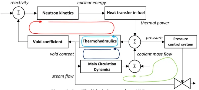
A BWR has significantly more complicated feedback and process relationship than earlier presented block diagrams above. The most important feedbacks in nuclear reactors are feedbacks through neutronics and thermohydraulics. A simplified BWR block diagram is presented in Figure 8.

Figure 8. Simplified block diagram for a BWR

In Figure 8 one can notice that there exist closed feedback loops in a BWR, of which several may cause instabilities. The red loop illustrates the feedback through neutronics, mainly caused by the void content which has the greatest impact on the neutron energy. The neutron energy and its relationship to nuclear reactions has been previously described in section Neutron reactions on page 5, and in section Power and reactivity control on page 8. The red loop can be observed studying the reactor power as a function of time.

nuclear energy

steam flow

void content coolant mass flow

pressure

Neutron kinetics

reactivity

∑ Heat transfer in fuel

thermal power ∑ Pressure control system Thermohydraulics Void coefficient Main Circulation Dynamics ∑

(33)

23

As an example, the processes that are involved in feedback through neutronics (red loop) can be determined from Figure 8. A reactivity perturbation as an input results in a power change, which in turn results in a change in the fuel temperature. Heat is conducted from the fuel pellet, through the fuel rod, and out into the coolant whose enthalpy changes affect the steam production, and thereby the void content, which affects the reactivity.

As an example, the processes that are involved in the feedback of the dark blue loop can also be determined from Figure 8. Main circulation pumps drive the coolant from the lower plenum, through the core, to the upper plenum. The coolant is then returned through the downcomer to the pumps. A perturbation in the pumps, resulting in a reduced recirculation, can cause the natural circulation to be the driving force. In natural circulation, the flow is driven due to a pressure difference. Due to boiling, the density is lower in the core than in the downcomer, which causes the mentioned pressure difference that drives the flow. A flow increase can in such a case reduce the void content and therefore decrease the pressure difference and in fact reduce the natural circulation.

The feedbacks are interconnected, which means for example that stability with respect to the neutronics feedback and instability with respect to circulation dynamics, can still result in power oscillations. This is due to the void content that makes a connection between the red and dark blue loop, see Figure 8.

Since different feedbacks may be dependent of each other, it makes it difficult to determine the true feedback that causes instabilities. Therefore, in order to investigate the stability of a NPP, it is necessary to set up a complete model of the neutron kinetics and thermal hydraulics. Such a model should include all inherent and engineered feedback effects. [20]

Boiling Water Reactor – plant components and plant

description

Conventional nuclear facilities consist of numerous systems and subsystems. Some systems are used for normal operation, while some are safety relevant systems. Minor disturbances are controlled by ordinary operating and control systems when there is no need to complete a reactor shutdown. Safety relevant systems, mainly of the RPV, can be divided into two subgroups: protection systems and shutdown systems. Protection systems monitor the reactor processes and initiate measures that may neutralize abnormalities. Shutdown systems are activated whenever a rapid reduce of reactor power is necessary, usually due to core cooling for some reason being insufficient.

Due to the scope of this project, only systems and their main components necessary for full power operation are described in this section. Therefore, the reader should keep in mind that many systems including many safety systems are absent. A general plant schematic is presented in Appendix 1.

(34)

24

The systems and components described in this section are based on plant documentation. The source is not public and cannot be revealed. System schematics are drawn based on ordinary flow charts and are for the reader to be used as an illustration to the corresponding system described.

Reactor vessel and internals

In order for a BWR to be a source of electricity, steam has to be created in the first place. Hence, the reactor tank is the most fundamental part of the whole nuclear power plant as it is responsible for the steam supply. The reactor core is located inside the reactor pressure vessel, RPV. The function of the core is to transfer heat created by nuclear fission of mainly uranium-235 to surrounding water. Steam is produced due to the heat absorption.

However, not all of the water undergoes vaporization in the core, which imposes generation of saturated steam. At the outlet of the core a mixture of moisture and steam is therefore obtained. It is necessary to separate the mixture in order to obtain as low moisture content as possible, so called dry steam to avoid erosion on the turbine blades and to enhance the efficiency of the turbines. The steam separator and dryers are installed in the upper section of the RPV.

The dry steam is transported to the main steam system, while the moisture is drained to the reactor recirculation system. The returning water is mixed with feedwater and further directed through recirculation pumps to the core, where the steam production process is repeated. [8] [9] The RPV is enclosed inside the reactor containment, which is a leak-tight and pressure-resistant construction. The containment prevents the release of radioactive substances to the environment in case of a damaged reactor tank but does also act as a shield protecting the tank from external events. All pipes passing through the containment are equipped with double isolation valves. [8] Even though it is desired for the steam leaving the reactor tank to be as dry as possible, it is technically impossible to remove all the moisture from the steam in the steam dryers. Some small fraction of moisture will therefore by carried by the steam and enter the main steam lines. The mass fraction of moisture in the steam that leaves steam dryers is called carry-over, whilst the mass fraction of steam that returns together with the water to the downcomer is called carry-under. Carry-over for a typical BWR is said to be 0.001, which means that about 0.1% of the mass of the steam leaving the RPV is moisture. [9]

Main pipelines inside reactor containment

The reactor containment is a construction surrounding the RPV and some of the primary process systems, such as recirculation systems including recirculation pumps. The steam generated in the RPV must be transported through the containment wall into the turbine facility TF, and likewise the feedwater must penetrate the containment to enter the reactor from the TF. [8]

(35)

25

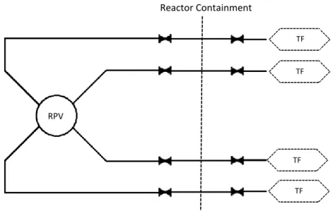
The distribution of the steam from the RPV to the TF is handled by the main steam system. During normal operation, the steam line system conducts steam from the reactor tank by four identical steam lines. The accumulated flow of the steam in the pipelines is greatest at full-power operation. The four pipelines carry the steam from the reactor tank to the TF through the reactor containment. Close to the containment wall each pipeline has isolation valves, one inner and one outer. The isolation valves function is to stop the flow of steam and isolate the containment if necessary. A schematic of the system is presented in Figure 9.

Figure 9. Schematic of the main steam line, and in opposite direction, the feedwater line

Turbine facility

Main steam system of the turbine facility

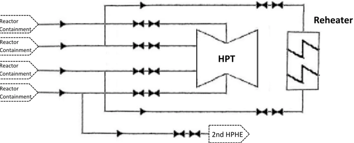
The main steam system of the turbine facility can be interpreted as a continuation of the steam lines that penetrated the containment wall. The purpose of the main steam system is to transport and divide live steam between the high-pressure turbine HPT and reheaters. A small fraction of the steam is under some operating conditions (e.g. full power) also directed towards the second high-pressure heat exchanger HPHE.

However, most of the steam enters the HPT. At the inlet to the HPT, each pipeline has two throttle valves positioned, one control valve and one intercept and emergency stop (quick closing) valve. It makes it possible to regulate or stop the flow of steam into the HPT if necessary.

The steam expands in the turbine, resulting in a pressure decrease. Due to the steam expansion, the humidity in the steam rises, while steam passes through the turbine. The outlet of the HPT is the beginning of the reheater system.

RPV Reactor Containment TF TF TF TF