ANALYSIS OF OPTIMIZATION POSSIBILITIES OF STRESS SCREENED ELECTRONIC
COMPONENTS
by Tamar Attia
All rights reserved INFORMATION TO ALL USERS
The qu ality of this repro d u ctio n is d e p e n d e n t upon the q u ality of the copy subm itted. In the unlikely e v e n t that the a u th o r did not send a c o m p le te m anuscript and there are missing pages, these will be note d . Also, if m aterial had to be rem oved,
a n o te will in d ica te the deletion.
uest
ProQuest 10783753
Published by ProQuest LLC(2018). C op yrig ht of the Dissertation is held by the Author. All rights reserved.
This work is protected against unauthorized copying under Title 17, United States C o d e M icroform Edition © ProQuest LLC.
ProQuest LLC.
789 East Eisenhower Parkway P.O. Box 1346
A thesis submitted to the Faculty and the Board of Trustees of the Colorado School of Mines in partial fulfillment of the requirements for the degree of Master of Science (Mathematics). Golden, Colorado Date K r ' t ! Golden, Colorado Date 1 Signed: y . / ? n v io l O JX .L& J Tamar Lisa Attia
Approved:
” r. Robert E .D Thesis Advisor
Dr. Ardel J. Boes Professor and Head, Mathematics Department
ABSTRACT
Stress screening is a generally accepted method in industry of being a cost effective way of removing early life failures of electronic components. The stress screening
procedure is the process of applying stresses such as humidity, power cycling, and heat to an electronic component to accelerate the age of the component to the point where early life failures will not occur. It is assumed that in some cases, it is cheaper to apply stress to screen out electronic components which will fail, than it is to repair and replace failures of the component in the field.
In 1985, a multiple stress, multiple component stress screening cost model was created by Lori Seward. The objective of the model is to trade off the costs associated with stress screening with the field failure costs incurred when no screening is performed. The model is unique in that it minimizes the cost of applying multiple stresses to
multiple-component subassemblies. This thesis is an analysis of the model. It shows the ranges of Weibull failure rate parameters for which the model is appropriate, since not all electronic components have failure rates which are high enough to necessitate stress screening. Two conditions were added to the model to enhance the range of its
application. One condition enables the model to indicate when an electronic subassembly (or component) should not be stress screened. The other allows the model to show when stress screening equipment should not even be purchased. Finally, this thesis provides a computer program which would enable a manufacturer to optimize the expected cost model.
TABLE OF CONTENTS PAGE ABSTRACT iii LIST OF FIGURES v LIST OF TABLES vi ACKNOWLEDGEMENTS vii DEDICATION viii CHAPTER 1 Introduction 1
CHAPTER 2 Explanation of the Multiple Stress, Multiple Component Stress
Screening Model 8
CHAPTER 3 Sensitivity Analysis 13
Implications of the Current Model Parameters 13
Sensitivity Analysis 18
Interpretations of the Sensitivity Analysis 26
Achieving Program Optimality 33
CHAPTER 4 Conclusions and Topics for Further Study 35
BIBLIOGRAPHY 37
APPENDICES 39
APP. A. Parameters Used in Original Model 39
APP. B. FORTRAN Optimization Program 41
LIST OF FIGURES
PAGE 1.1 Typical Failure Rate Curve (Miller, e t al., 1990) 4
2.1 Field Failure Function 16
2.2 In-House Failure Function 17
2.3 Unit 1 Failure Probability Function 19
3.1 Unit Three Failure Probability Function at Optimality 29 3.2 Unit Five Failure Probability Function at Optimality 30 3.3 Unit Eight Failure Probability Function at Optimality 31 3.4 Unit Nine Failure Probability Function at Optimality 32
LIST OF TABLES
PAGE
1. Sensitivity Analysis 23
2. Stress Levels of Optimized Units 28
ACKNOWLEDGEMENTS
My deepest thanks to Dr. Woolsey for providing an interesting and educational experience at the Colorado School of Mines. Thanks for the guidance, encouragement, and skills to solve "real-world problems" with Operations Research.
Thanks to the members of my thesis committee, Dr. Barbara Bath, Dr. Ruth Maurer, Lori Seward, and Dr. Woolsey, for assisting me and teaching me while I was working on my thesis.
Thanks to my friends in the Guild who helped me and supported me.
DEDICATION
This thesis is dedicated to my parents, my husband, and my expected child.
CHAPTER 1 Introduction
There is a great deal of evidence that stress screening is a cost effective method for removing early life failures from a population of electronic components, thereby
increasing the reliability of units to be sold. However, not all components exhibit a substantially large or small early life failure probability to justify stress screening. When considering cost optimization models for stress screening, it is necessary to recognize that not all components will benefit from this process. There is a range of failure parameters for which stress screening is cost effective though. For these cases, it is useful to note that the difference between finding a global minimum and a local minimum in an optimization model is a difference in savings to industry. In the literature search conducted for this research, no computer packages were found which will assure global optimality for nonconvex nonlinear optimization models.
Nachlas, Seward, and Binney, 1986, solved such a nonconvex nonlinear optimization model with a package called GINO, which uses the reduced gradient algorithm to solve nonlinear optimization problems. A solution was obtained with no assertion of optimality. A different solution is obtained by the program this thesis provides. While this solution is not the global minimum to the expected cost equation, it appears to be the best solution within the variable bounds given.
Seward, 1985, developed the multiple stress multiple component cost optimization model which is the basis of this thesis. The model is unique in that it minimizes the cost of applying multiple stresses to multiple-component subassemblies. This thesis is an
analysis of the model. The Seward model was shown to be an effective tool in minimizing the cost of applying multiple stresses to subassemblies by determining optimal stress levels and the time stress should be applied. This thesis added two conditions to the model to enhance the range of its application.
Chestnut, 1967, and Nahmias, 1989, briefly discuss the impact of poor reliability. The impact of poor reliability on the consumer is the inconvenience of purchasing faulty equipment and the unavailability of the needed equipment. The impact of poor reliability on the manufacturer of electronic components is the price of returning failed units to repair them, and the loss of sales due to a damaged reputation.
Unpredictable reliability, therefore, is a problem for both consumers and
manufacturers. Due to the probabilistic nature of failure patterns, it is difficult to predict how goods will fail. However, there is enough information in the field to be able to model items according to some well-known distribution functions and use this
information to improve reliability, thereby reducing costs for all concerned. Chestnut, 1967, Nahmias, 1989, and Nachlas, et. al, 1984, provide methods and examples.
To date, most of the electronic components studied have shown a Weibull failure distribution (Nahmias, 1989.) Nachlas, et. al., 1984, and Nachlas, et. al., 1985, provided results of experimentation confirming failure rates of electronic components to be Weibull distributed. This means that upon analysis of failure rates of components, (where failure rate is the "measure of likelihood that if a component has survived up to time t, it will fail in the next instant of time" (Nahmias, 1989),) the data can be fit to a
Weibull distribution curve. Chestnut, 1967, also stated that "evidence shows that the failure rate of most electronic parts decreases with increasing time," which is a primary reason for using the Weibull distribution.
Nachlas, Gruber, and Wiesel, 1984, presented a paper showing that errors in Weibull parameter estimation had a relatively little effect on determining machine reliability. While it may be true that some errors have relatively little effect on determining reliability, this thesis showed that the resulting cost of the optimization model created by Seward is parameter dependent. Therefore, there is a necessary level of reliability in parameter estimation to assure proper results when using the model.
Sensitivity analysis performed in this thesis gives insight into the degree of effect that changes in the parameters have.
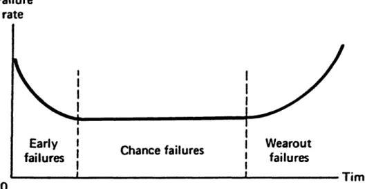
Generally, failure rates or the life cycle of electronic components can be modeled by the "bathtub curve" (Miller, et. al., 1990). The early life (known as the infant mortality or bum-in stage) is where the failure rate starts out high and decreases until it reaches a relatively constant period. The constant period is known as the useful life of the product (which includes the length of a mission or the time until obsolescence of an assembly, denoted by "T" in this thesis.) At the end of the useful life, the failure
distribution may change as the wearout phase begins. This is represented by the upward slope at the end of the bathtub curve. (See Figure 1.1.) The Weibull distribution is unique in that it represents items with either increasing or decreasing failure rates for units which exhibit signs of aging (Nahmias, 1989, and Miller, 1990).
Failure rate Early failures W earout failures Chance failures Tim e 0
Figure 1.1 - Typical Failure Rate Curve (Miller, e ta l, 1990)
After confirming that failure data is exhibiting a Weibull failure rate pattern, there are two parameters to be estimated in the Weibull distribution: a , the scale parameter, and P, the shape parameter. Nachlas, Binney, and Gruber, 1985, used both the method of maximum likelihood, and regression analysis to determine the parameter values in their experimentation. A brief explanation of these two methods follows to explain the processes which are commonly used to approximate Weibull parameters in experimentation with failure rates.
The method of maximum likelihood is the most widely accepted approach for Weibull parameter estimation (Miller, et. al., 1990.) This method looks at the values of a random sample, which in this case would be time to failure of observed electronic
components, and then chooses as the parameter estimate that for which the probability of obtaining the observed data is a maximum. If x 1,x2, are the values of a random sample from a Weibull population, the parameters a and p are found by taking the log of likelihood function
L(a,p)
a, P)
and then differentiating it with respect to a and p and solving the equations by equating them to zero.
Plesser and Field, 1977, and Nachlas, e t al, 1987, used regression analysis in their experimentation. Regression analysis is the method of fitting a straight line or a curve to a set of data and then observing how closely the line or curve, with the parameters chosen, approximates the data.
All of the parameters in the model must be estimated before using the stress screening model. The object of stress screening is to compress the time that failures occur in the early failure period so that the units can more readily reach their useful life period, where the probability of failure is constantly fairly low. Stress screening is a generally accepted method of accelerating the time of these early life failures. By applying external forces such as heat, humidity, and voltage before a unit is assembled and marketed, early life failures can be induced and screened out in-house, thus
increasing the reliability of the unit once it is sold. This implies a savings to the company as it is cheaper to repair components and subassemblies in-house and before assembly than it is to return and repair entire units once they are sold. Kuo and Kuo, 1983, Nachlas, et. al., 1985, Reda and Brown, 1976, and Rue, 1976, confirm that stress
screening is a cost effective method for removing early life failures after determination of optimal burn-in periods.
There is a cost to applying these external age acceleration forces to components. The model developed by Seward, 1985, is a general cost model for use in selecting a stress regimen for a multiple stress assembly-level stress screen. The objective of this model is to trade off the costs associated with stress screening with the field failure costs incurred when no stress screening is performed. The model is set up to represent the following:
Expected total cost of stress screening= (Cost of field failure * probability of field failure)
+ cost of stress application
+ (cost of in-house failure * probability of in-house failure)
1.1
The original model took the form of an unconstrained, non-convex, nonlinear programming problem. Using a generalized reduced gradient method, a solution was obtained with no assertion of optimality. This thesis provides several useful insights into the model. It explains how two adjustments to the model will enhance the range of its applications, and it also provides a method for achieving optimality of the expected cost model within the variable bounds given.
CHAPTER 2
Explanation of the Multiple Stress, Multiple Component Stress Screening Model
For the purpose of example, a five-component subassembly with failure
probabilities corresponding to a series network (i.e., if any component fails, the unit no longer functions) was examined. Assuming that failure of any of the components is independent of the failure of another, the reliability of the unit can be measured as the probability that all components i with mean time to failure tt will survive after some time x, and is known as R(x).
The symbolic representation of the reliability of a series system is:
(Nahmias, 1989, and Miller, Freund, and Johnson, 1990)
As explained in Chapter 1, it is appropriate to represent electronic component failure probability with the Weibull density function F(x);
Symbolically, R(x) = P {minfo, t2, ..., t5) > x} = P { r1> x , r 2> x ,... r5> x } = P U > x) * P{r2 > x) * . . . * P{r5 > x) 2.1 2.2 F ( x ) = l - e i=x Z -a x j = t J 2.3
-at J
where each e j is P{ti > x) as in Eqn. 2.1. a and p are the Weibull parameters (see
Chapter 1) and t is the variable, time.
By applying the stresses Slt humidity, S2, voltage, and S3, temperature, each component will experience a different amount of acceleration of its equivalent age (power-on hours) x.
Xy= 0/(*S'i,iS'2>*S'3)f 2.4
where aj(Si) is the acceleration factor associated with component j and stress duration t. Nachlas, et. al., 1985, equates
a fti) = Gxp(gjti(Si)) 2.5
where gjti is the stress function associated with stress i and component j. Eqn. 2.6 is defined in the above reference as a best linear fit of the logarithmic function gy j(5,).
d j i + hj'iSi. 2.6
So with acceleration, x becomes:
dJ . i + h J .is i
% = te 2.7
Remember, t is the amount of time that stress is applied. Nachlas, et. al., 1985, addresses the question of how to compute the aging acceleration that results from the simultaneous application of multiple stresses.
The conditional probability of field failure of the unit before the end of its useful life T, given in-house survival up to time T
= P ( t'£ T + x \t'> x ) 2.8 P(t'Z T + x ,t '> x ) P(t'> x) P { x < t'£ T + x ) P(f'>x) 2.9 2.10 F(x+T)-F(x) - l t 1 -F (x) ^*AA F(x+ T)-F(x) -R(x) 1 - exp(-a(x+ 7 ^ ) - 1 + expHxr^) ^ ^ *P(V) - exp(-a(T+i f )+ exrt-ottP) ^ exp(-otr^) = 1 - exp(-a(x+ T f + axp) 2.15
Using the same explanation as in Eqn. 2.3, for a five component system, Eqn. 2.15 becomes
1 - expf £ - a / x + r f ‘ + £ a , / ' | 2.16
In order to clarify the model, define the following: Pi = constant cost of running each stress machine i
<7,- = cost of applying each stress at the specified stress level Cj = cost of in-house failure
CF = cost of field failure E(c) * expected cost
The probability of in-house failure is simply
F(x). 2.17
The cost of applying the stress is
X A + X q i( S i- S oi)t 2.18
i = i » = i
E(c) of in-house failure is
Cj*F(t) 2.19
E(c) of field failure is
CP*F(T + t | t) 2.20
Combining all the above information leads to the mathematical representation of the multiple stress, multiple component stress screening model (Seward, 1985).
The problem is: minimize
E(c)=CF\ l - exp t
expJ^X
d j'i+
+
r j + X_ a/r exp^X
dh i+fy.sjl
+ C/j 1 - exp
X -a,
\j=i s.t. 0 <>t<>UtSoi < Si <> Ui for i = 1,2,3
2.21
where Ut is the upper bound given for the time stress is applied, Soi is the level of stress equivalent to zero acceleration, 5, is the level of stress applied, and Ui is the upper bound on the amount of stress which can be applied. (Seward, 1985) provides a more detailed explanation of how the model was developed.
CHAPTER 3
Sensitivity Analysis and Achieving Optimality
Implications of the current model parameters
Implicit in describing the usefulness of stress screening is the fact that the
manufacturer’s cost with the stress screening should be less than the cost when no stress is applied. This was not the case for the components with Weibull parameters such as those in Nachlas, et. al., 1986. (Please see Appendix A for the original model
parameters.) This section will explain how the solution to the multiple stress, multiple component stress screening model Eqn. 2.21 is affected by these parameters.
Initially, a solution to the stress screening expected cost equation was obtained (Nachlas, et. al, 1986) by the software package GINO, using the original parameters (Appendix A):
51 (amount of humidity applied) = 75% 52 (amount of voltage applied) = 2 CYC/HR 53 (amount of temperature applied) = 350°K
t (time that stress is applied) = 22.44 hrs. E(c) (expected cost) = $.563 per assembly
It is of interest for manufacturers to see how much money they will save by using stress screening. It is expected that:
Without applying any stress, and using the same set of alpha and beta parameters, the industrial cost of unit failure is simply the cost of field failure times the probability of field failure. This is computed as follows:
(Note that T is the useful life of 2000 hours of the system, and a y, (3; are the Weibull parameters listed in Appendix A.)
Comparing this result to the original result, implies that for this assembly,
In other words, this result shows that stress screening would not be cost effective for a company which has components with these failure rate parameters, and a useful life of 2000 hours. However, GINO does not ascertain that its result is optimal.
This thesis contains a program (Appendix B) which searches over all variable values and prints each expected cost as it appears, if lower than the previous one found. While this program is perhaps not as computationally efficient as some software
packages, it insures that the optimal answer (to the closest hour), within the bounds given, is found. The result was:
= 100(1 - exp[(2.25T'4 + 4T AS + 6.25T*5 + 8.25T55 + 9 .4 r>6)10^1) = $.1886 per assembly
51 (humidity) = 25% 52 (voltage) = 2 cyc/hr S3 (temperature) = 298°K t (time the stress is applied) = 300 hrs
E(c) = $.3586 per assembly
Note that this solution is better than the one found by GINO but still implies it is not cost effective to screen components which have those Weibull parameters and that useful life. The implication of this last result is that the most cost effective solution is to apply the equivalent of no acceleration (5, at its lower bound) and leave units in-house as long as possible (t at its upper bound). This is not a reasonable result as will be explained in this section.
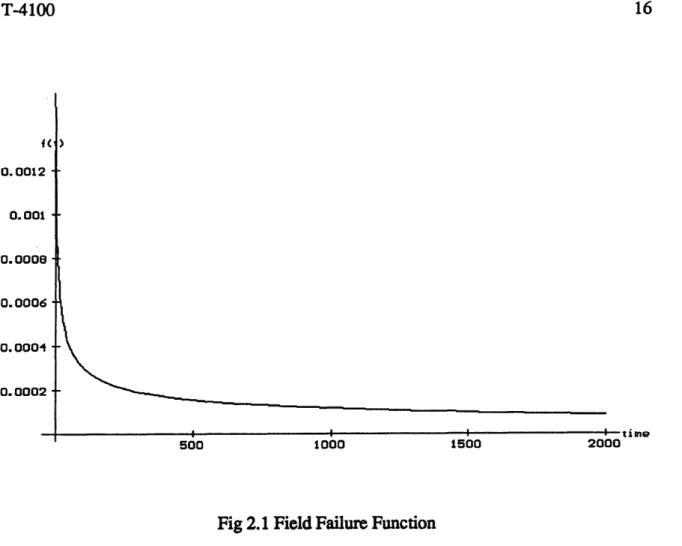
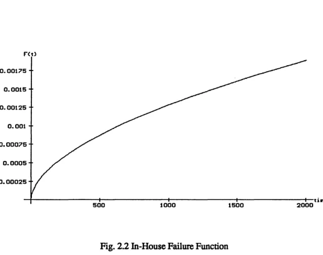
In situations where stress screening is appropriate, the field failure function is decreasing, Fig 2.1, because the probability of field failure is reduced as the in-house time of stress applied is increased. The in-house failure function for such a unit is increasing, Fig. 2.2, because the longer stress is applied in-house, the higher the
probability of in-house failure. One would expect that the two functions would intersect at a point before the amount of time that stress is applied reaches its upper bound. This is because this point represents the tradeoff when screening reduces failures to the point where it is cost-effective to put the product on the market.
0.0012 -0.001 ■ ■ o.oooe 0 .0 0 0 6 0 .0 0 0 2 ■ -t i n e 2000 1500 1000 500
Fig 2.1 Field Failure Function
F< t) 0.0015 0.00125 - ■ 0 . 0 0 1 - ■ 0 .0 0 0 5 * * 0 .0 0 0 2 5 - • 500 1000 1500 2000
Fig. 2.2 In-House Failure Function
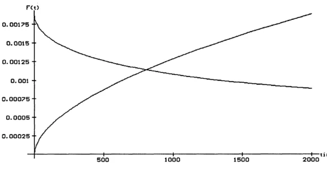
The current solution says do not apply stress but keep the product in-house as long as possible. This result occurs because the model is considering only the expected cost of failure, not the benefit received when the product is sold. Since, for this unit, there is no benefit from applying stress for a time which is within the original bounds of t (see Fig. 2.3), the model can only indicate that the cheapest cost will occur when t is left in-house as long as possible. This result is not a practical one for the manufacturer though because units with very low probability of failure should be ready for market very early on, if not immediately, to maximize profits from sales. This model is not intended to maximize sales profits though, only to reduce failure costs. Therefore, it is necessary at this point to adjust the model in such a way that it will indicate, in situations like this, that screening is not needed, and the product is ready to be sold. This change will be explained in the following chapter.
Sensitivity analysis
It was revealed that stress screening is not cost effective for all components and seems to be dependent on the Weibull (failure rate) parameters. For example, the
parameters of the component given in Nachlas, et. al., 1986 were such that the probability of failure was very low (close to zero, in fact) and the optimal solution was to forego the cost of screening.
As the multiple stress multiple component model (Seward, 1985) is applicable to any type of component, it is useful to show which ranges of parameter values will justify stress screening. The model can then be used to determine the amount of stress and the time it is applied to determine optimal cost effectiveness.
Rt> 0.00175 - ■> 0.0015 - ■ 0.00125 - ■ 0 .0 0 1 -• 0 .0 0 0 7 5 -0 .-0 -0 -0 5 - ■ 0 .0 0 0 2 5 - ■ time 2000 1000 1500 500
Fig. 2.3 Unit 1 Failure Probability Function
This graph is the intersection of the field failure probability function and the in-house probability function for the original unit.
Since it is generally accepted in industry that electronic components experience a decreasing failure rate, it is therefore appropriate to use the Weibull distribution with t > 0, a > 0,0 < P < 1 to model these rates (Miller, et. al., 1990). As previously discussed, it is possible to have parameters representing such a low probability of failure that
screening is not cost effective. Likewise, it is possible to have parameters representing such a high probability of failure that stress screening is irrelevant as cost will always be
(CF * Probability of field failure) 3.2
+ (Cj * Probability of in-house failure) + nominal cost of applying stress
where the probability of failure = 1. In other words, the cost will be constant. The question which remains then, is for what range of parameters is stress screening
appropriate. It will be assumed that the useful life of 2000 hours, representing the length of a mission, or the average time before failure or obsolescence of the unit, will be
constant. However, the useful life also affects the amount of time stress is applied. Since T, the useful life, is constant for this example, sensitivity analysis on the parameters a and p is therefore the appropriate method for determining the ranges for which screening is appropriate.
Since a and p were arbitrarily picked, it will be assumed for the purpose of this illustration that each a y and py change only in order of magnitude to the parameters in the original paper (Seward, 1985). Therefore, sensitivity analysis will be performed by changing only the powers of these variables.
Two conditions were added to the model prior to performing sensitivity analysis. The first one indicates when the probability of failure is so low that the units need not be screened. When optimality occurs at 5, = Si0 (i.e., stress is at its lower bound) it will be assumed that t (acceleration time) = 0. Since t is the amount of time the unit is stressed, it would not make sense to have t at anything but zero when the stresses are at the level of stress equivalent to zero acceleration. It is also sensible that when the probability of field failure is very low, the product is ready to be sold. It should be remembered that the model does not maximize profit to be gained when the product is sold, it only minimizes the cost of failure in preparation for sale time. The condition added should indicate when the product is ready to be sold.
The second condition considers the fact that a company may be using the model to indicate whether it is cost effective enough to stress screen that they would want to buy stress screening equipment. By assuming that at t=0, there is no constant cost of stress screening, a company can determine what its cost with stress screening would be
compared to its cost without. For example, the original parameters showed the minimum to occur at:
51 (humidity) = 25% 52 (voltage) = 2 cyc/hr S3 (temperature) = 298°K t (time the stress is applied) = 300 hrs
Optimality with the two new conditions would occur at: 51 (humidity) = 25%
52 (voltage) = 2 cyc/hr S3 (temperature) = 298°K t (time the stress is applied) = 0 hrs
E(c) = $.189 per assembly
because of the fact that there is no cost of applying stress at t-0 . Whereas the old solution said to keep stress at its lowest level and let the unit run in-house as long as it can, the new solution says do not apply stress. The resulting cost is cheaper, and the product has 300 more hours available to be sold. As Table 1 shows that the probability of failure for this unit is very low, therefore it seems reasonable that these units do not need to be screened, and is ready to be sold. Table 1 shows the probabilities of in-house and field failures for various alpha and beta parameters, as they appear at optimality.
TABLE 1 Sensitivity Analysis
Sensitivity analysis on a and (3 parameters of units different only in the order of magnitude with those in Appendix A.
Note: Probabilities are rounded to three decimal places.
UNIT a, ft PF(failure) Pjifailure) Expected rat Si at
# Optimal optimality optimality
Cost 1* 2.25* 10-6 .4 0 .017 .189 0 Sx= 25 4*10-* .45 S2= 2 6.25*10-* .5 S3= 298 8.25* 10"* .55 9.4*10-* .6 2 2.25*10-* .04 0 0 .005 0 Sx= 25 4*10-* .045 S2- 2 6.25*10-* .05 03 IICO 00ON 8.25*10-* .055 9.4*10-* .06
UNIT (Xi p, PF(failure) P,{failure) Expected rat # Optimal optimality Cost 2.25x10"5 .4 .007 .03 1.14 13 4x10~5 .45 6.25x10⁻⁵ .5 8.25xl0'5 .55 9.4xl0"5 .6 2.25x10"5 .04 0 0 .05 0 4xl0"5 .045 6.25x10⁻⁵ .05 8.25x 10"5 .055 9.4x10⁻⁵ .06 2.25x KT4 .4 .034 .539 5.39 72 4x10^ .45 6.25X10⁻⁴ .5 8.25X10"4 .55 9.4x KT4 .6 Si at optimality 75 S 2=
8
53=350 5X= 25 S2= 2 53=298 5X= 75 52= 8 53=350UNIT
#
6
7
a i P.* PF(failure) Pjifailure) Expected rat 5, at Optimal optimality optimality
Cost 2.25a: 10-4 .04 .004 0 .04 0 $j= 25 4JC10-4 .045 $2= 2 6.25a: 10-4 .05 $3=298 8.25a: 10-4 .055 9.4* 10"4 .06 2.25* 10-4 .004 0 .003 .226 0 $j= 25 4*10-4 .004 52= 2 6.25* 10-4 5 $3=298 8.25* 10-4 .005 9.4* 10"4 .005 5 .006 2.25a: 10"3 .4 .176 1 23.76 30 $!= 75 4*10~3 .45 $2= 8 6.25* 1(T3 .5 $3=350 8.25* 10'3 .55 9.4* 10'3 .6
UNIT a, ft PF{failure) Pjifailure) Expected rat 5, at
# Optimal optimality optimality
Cost 9 2.25a: KT3 .04 .002 .045 .52 6 S t = 75 4jc 10-3 .045 <S2= 8 53=350 6.25a: KT3 .05 8.25a: KT3 .055 9.4a: 10~3 .06
* Unit 1 is the unit whose parameters are in the original model.
Observe that for components with Weibull parameters changed only by a power of ten to those in the paper by Seward, 1985, only units 3, 5, 8, and 9 would benefit from stress screening. This determination was made by simply noting that when t is not zero at optimality, this implies that the unit will benefit from stress screening, and if t = 0 , this implies that the unit will not benefit from stress screening. So, the remaining units
(original example included,) which have failure probabilities of either 0 or 1, as explained in Chapter 2, will not benefit from stress screening.
Interpretations of the sensitivity analysis
As mentioned in the previous section, not all units will benefit from stress
screening. Table 1 shows that units 1 (the original example), 2 , 4 , 6 , and 7 have such a low probability of failure that stress screening is not appropriate. Also, as was mentioned in the previous section, if both PF, the probability of field failure, and Ph the probability
of in-house failure, are very high, the cost would become constant, indicating the amount of stress applied is irrelevant. This will not be the case if only Pt is high though, as with Unit 8 .
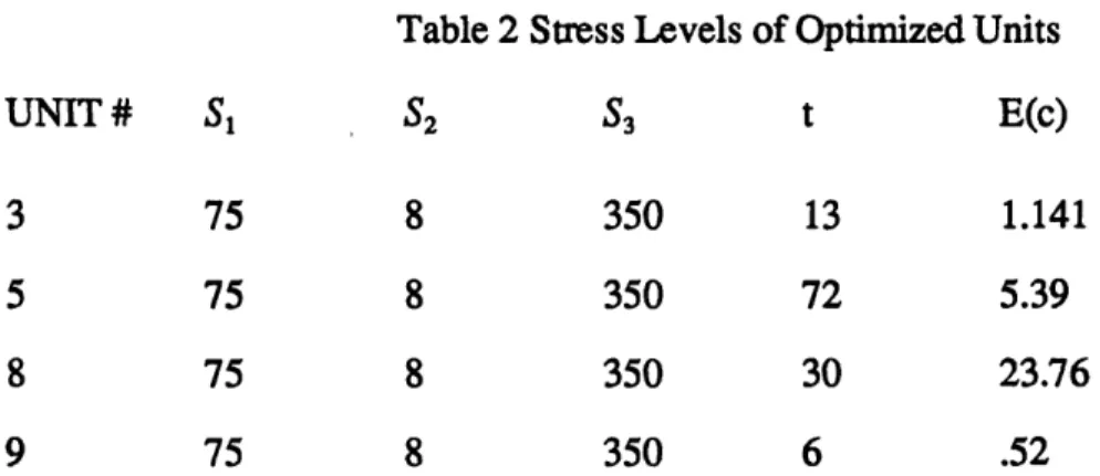
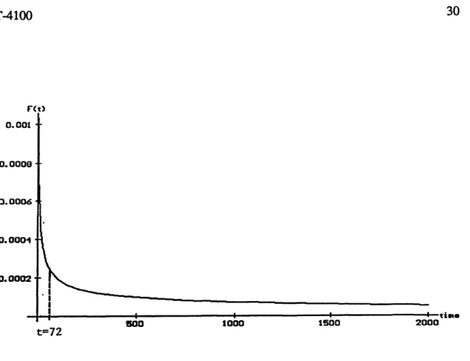
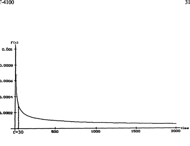
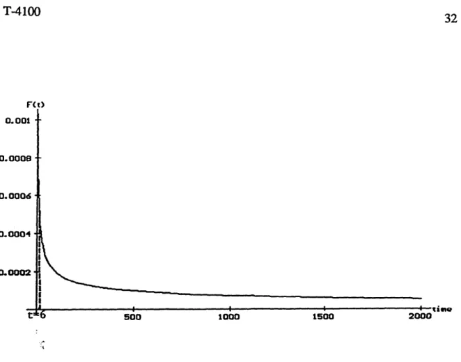
Pj is an increasing function with respect to stress because the longer stress is applied the higher the probability of failure is in-house. PF is decreasing over time because as the failure rate of these units is a decreasing one, the longer the unit is on, (before the wearout period begins) the lower the probability of failure will be. And of course, the longer stress is applied, the lower yet PF will be. Unit 8 has the highest probability of in-house failure, but since P, is an increasing function (with respect to time) and PF is a decreasing function, the unit should definitely be stressed because as t increases, the probability of field failure, and therefore the cost will decrease. Units 3,5, 8 , and 9 are the units which will benefit from stress screening, due to the nature of their probabilities of failure. These units were run through the optimization program to observe trends in attaining optimality. The result was is shown in Table 2.
Table 2 Stress Levels of Optimized Units UNIT# Si Si S3 t E(c) 3 75 8 350 13 1.141 5 75 8 350 72 5.39 8 75 8 350 30 23.76 9 75 8 350 6 .52
Observe that in Figure 3.1 - Figure 3.4, that optimality appears to occur at the point where the failure rate curve stops decreasing rapidly. Intuitively, this is a reasonable result because stress screening is designed to compress the early life failures into a shorter period of time, so that fairly reliable units can be put on the market and sold (Nachlas, et. al., 1985). The fact that all of the expected costs of the units reached optimality at the upper bounds for the stresses implies that for this set of costs and variables, stress screening is very cost effective as the most benefit is received from the largest amount of stress. Further sensitivity analysis could be done to show for what costs and variable ranges optimality will still occur at the upper bound of stress for these components. For example, if unit 3 is stressed at the following levels
51 (humidity) = 100% 52 (voltage) = 35 cyc/hr S3 (temperature) = 400°^ t (time the stress is applied) = .128 hrs
the expected cost would be $.58/unit, as opposed to $1.141/unit However, there are several reasons why these bounds may be impractical. The stress equipment may not be able to reach those stress levels. The unit may not be able to withstand those levels of stress. Finally, the accelerated age o f this unit may have reached the wearout phase of its life. r<o 0.00004 2000 1000 1500 500
F<t> 0.001 -0 .-0 -0 -0 8 -0 .-0 -0 -0 4 0.0002 2000 1500 1000 500 t = 7 2
F<«) 0.601 o.o o o q -3 .0 00 6 ■ 0 .0 0 0 4 0.0002 2000 1500 1000 500 =30
F(t> 0.001 -0 .-0 -0 -0 8 -0 .-0 -0 -0 6 • ; 0.0002 2000 1500 1000 5 00
Assuming the bathtub curve model applies to the life cycle of this unit, there is a period of time when the unit is expected to start failing again. Observe that the
accelerated age of Unit 3 with the new upper bounds is \ t = £ t exp X d jti + h jtiSi
7 = 1 V = 1 = 72,397 hours
(as opposed to 3,618.48 hours for the original upper bounds). Since stress screening is only concerned with early life failures, it was not necessary to model, but necessary to remember, the fact that there is an end-of-life period when failures will start increasing. If, for example, the alpha and beta parameters change after the unit is 72,000 hours old in such a way that represents an increasing failure rate of the unit at this point, it is obvious that these new stress levels would not be appropriate. However, since the cost was decreased with these new bounds, it seems that a company manufacturing units 3,5, 8 , and 9 would want to investigate how much further the stress levels can be increased, while leaving enough useful life so as to benefit from sales of the product.
Achieving Program Optimality
As discussed in the previous section, there is a point, in determining stress levels, where the payoff to be received from selling the product overtakes the need to increase the reliability of the product. While applying massive amounts of stress in a very short time might be the most cost effective way to improve the reliability of the product, the equivalent life of the product after the stress is applied may be so high that it would actually be at the point in its life where it can expect to start failing again. This model
does not include the fact that there is a point in the components life where it is expected to start failing again, because it is assumed that there is a known upper bound of time that industry wants to apply stress. Of course, this upper bound must be mathematically computed by industry, by seeing the point of intersection between the cost savings function (of improving reliability) and the sales profit function.
The program used to solve the model assumed that the upper bounds of the four variables (time, humidity, voltage, and heat) were analytically predetermined. The program also assumed that accuracy, to the nearest hour of time was sufficient. This was assumed in the interest of efficiency in running the model. In an industrial situation, greater accuracy of time would probably be required.
The program is written in FORTRAN. To use the program, the program must be entered, and the appropriate alpha and beta parameters must be entered on the lines beginning with "data A" and "data B." The lines beginning with "Data D" and "Data H" are the acceleration parameters in the stress function. "Data SZ" is the lower bound for the stress values. The final change which may be needed is in the first four "do" loops, which show the ranges to search over the four variables.
The program performed a four-dimensional search over all the variables and noted as each better solution was obtained. Therefore, it can be assured (with the
aforementioned conditions) that since every combination of variables was considered, that the optimal answer was found.
CHAPTER 4
Conclusions and Topics For Further Study
This thesis has outlined the many ways in which the multiple stress, multiple component stress screening model can be used to achieve optimum cost-effectiveness for industry. When the probability of field failure is very close to 1, the model indicates that again, stress-screening is not cost effective as cost will become constant-valued. When the Weibull parameters are such that the probability of failure is close to zero, screening was shown not to be cost effective as there is no early life in which to induce failures.
A condition was added to the model that for 5, = Si0 (stress at the level equivalent to zero acceleration), t necessarily is 0. This condition is necessary as the model does not take into account profits to be gained from sales. Therefore, for units with very low probabilities of failure, a manufacturer needs to know that the product is ready to be sold. Another condition was added to the model that says that for t=0, there is no constant cost of applying stress. In the initial stages of production, this will help a manufacturer know whether or not it is cost effective to buy stress screening equipment.
For the case where probability of failure is moderate, the model showed stress screening to be cost effective. A manufacturer could then do sensitivity analysis on various parameters and costs, and use the model to determine what levels of reliability would achieve maximum cost effectiveness. It was shown, for example, that when optimality occurs with stresses at the upper bound, this tells the producer that increasing stress levels will probably decrease the expected cost. However, this result may not be
reasonable. The ability of the assembly to withstand such levels of stress must be investigated. The stressing equipment may need to be changed to apply higher levels of stress. Also, since acceleration increases the age of the assembly, it must be determined what affect the resulting sacrifice of useful life would have on sales profits.
There are several other conditions which must be imposed before determining what the optimal answer to the model will be. The upper bound on time of stress application must be predetermined as it affects acceleration of the unit. The necessary degree of accuracy of time must be predetermined as expected cost could approach optimality as time in incremented in smaller intervals. However, this will have an affect of the amount of time the optimality program takes to run. The useful life of the assembly and the costs of in-house and field failure must also be predetermined. This thesis then provides a method for optimizing the model by calculating the optimal levels of stress and the optimal time of applying them necessary to achieve minimum cost.
BIBLIOGRAPHY
Chestnut, Harold; Systems Engineering Methods: John Wiley and Sons, Inc.; New York, 1967.
Kuo, Way, and Yue Kuo; "Facing the Headaches of Early Failures: A State-of-the-Art Review of Burn-In Decisions; Proceeding of the IEEE: Vol. 71, No. 11, November
1983.
Miller, Irwin, John E. Freund, and Richard Johnson; Probability and Statistics For Engineers: Prentice Hall; New Jersey, 1990
Nachlas, Joel A., Blair A. Binney, and Stephen S. Gruber, "Aging Acceleration Under Multiple Stresses"; 1985 Proceeding Annual Reliability and Maintainability Symposium: January 1985. pp. 438-440
Nachlas, Joel A., Stephen S. Gruber, and Harry Z. Wiesel; "Sensitivity in Weibull System Reliability Models"; 1984 Proceeding Annual Reliability and Maintainability
Symposium: January 1984. pp. 428-433.
Nachlas, Joel A., Lori E. Seward, and Blair A. Binney;" Multiple-Stress Assembly-Level Stress Screening," Proceedings of the Annual Reliability and Maintainability
Symposium: Las Vegas, Nevada; January 1986. pp. 40-43.
Nahmias, Steven; Production and Operations Analysis: Irwin; Boston, MA; 1989. Plesser, Kenneth T., and Thomas O. Field; "Cost-Optimized Burn-In Duration for
Repairable Electronic Systems"; IEEE Transactions on Reliability: Vol. R-26, No.3; August 1977. pp. 195-197.
Seward, Lori E.; “Cost Efficient Multiple Stress, Multiple Component Stress Screening"; VA Tech, VA; 1985.
Reda, M. R., S. G. Brown, and K. L. Menze; "High Temp. Burn-in and its Effects on Reliability"; 1976 Proceeding Annual Reliability and Maintainability Symposium:
1976. pp. 72-74.
Rue, Herman D.; "System Burn-In for Reliability Enhancement"; 1976 Proceeding Annual Reliability and Maintainability Symposium: 1976. pp 336-341.
APPENDIX A
Parameters Used In the Original Model
Weibull parameters Oj = 2.25*10“6 0 2 = 4.0*10"* <X3 = 6.25* KT6 a 4 = 8.25* 10"6 a 5 = 9.4*10"* Stress Function parameters
rfn = -.03875 d12 = -.304 d13 = 38.915 421=-.0365 ^22 = —.276 ^ 23 = 38.915 = -0 3 4 5 d$2 = —»28 d33 = 38.915 Pi = .40 p2 = *45 P3 = .50 p4 = .55 Ps = *60 *n = 1.55*10,-3 * 12 = .152 * 13 = -11596.9 * 21 = 1.46xl0'3 *22 = * 1 3 8 /** = -11596.9 *31 = 1.38x10* * 3 2 = - 1 4 * 33 = -11596.9
d4\ = -0 3 8 d42 = -.31 d43 = 31.133 dsi = “ 037 ^52 =-.31 rf53 = 31.132 Cost parameters
CF = $100 per item field failure Cf = $1 per item in-house failure Pi = .1 ($/item)
Pi - -07 p 3 = .05
Nominal stress levels
*S01 = 25% S02 = 2 cycles/hour Bounds h4l = 1.52* 10"3 /i42 = .155 ^43 = -9277.5 /i51 = 1.48jc10"3 /z52 = .155 /*53 = -9277.5
= 9x l 0 -7 ($/stress unit - time unit) q2 = 8JC10-4
= 2.25;tl0"4
S03 = 29S°K
APPENDIX B
FORTRAN Optimization Program
C THIS PROGRAM FINDS BEST ANSWER FOR E(C) C DEFINE VARIABLES
REAL t,Tecn, TEC, EC1, EC2, EC3, S3, sm2,P<3)
INTEGER S2, J, I, CF, Cl
real A<5>, D<5,3), H(5,3), B<5>, SZ(3), Q(3),EA(5) data A/2.25E-06,4.0E-06,6.25E-06,8.25E-06,9.4E-06/ DATA B/.4,.45,.5,.55,.6/ DATA P/.1,.07,.05/ DATA Q/.0000009,.0008,.000225/ DATA D /-.03875,-.0365,-.0345,-.038,-.037.-.304,-.276,-.28,-.31, * -.31, 38.915, 38.915, 38.915, 31.132, 31.132 / DATA H /.00155,.00146,.00138,.00152,.00148,.152, .138, .14, * .155,.155, -11596.9, -11596.9, -11596.9, -9277.5,-9277.5/
C DEFINE LOWER BOUNDS FOR STRESSES
DATA SZ /25, 2, 298/
open(uni t=15,f iIe='EXPTCOST.dat',status='NEW', access^'append')
C DEFINE COSTS
CF=100
Cl=1
C DEFINE USEFUL LIFE
BT=2000 TECN =500
C LOOP THROUGH APPROPRIATE RANGES OF THE FOUR VARIABLES
DO 10 T=1,300,1 DO 20 S1 =25,75,1 DO 30 S2=2,8,1 DO 40 S3=298,350,1 EC2 = P(1) +0(1)*(S1-25)*T ♦ P(2)+Q(2)*(S2-2)*T+P(3)+Q(3)* * <S3-298)*T
APPENDIX B cont’d.
C THIS "IF" STATEMENT WILL DETERMINE THE EXPECTED COST WITHOUT THE SUNK
C COST OF OWNING STRESS SCREENING EQUIPMENT
IF <T .EQ. 0) THEN EC2 = 0 END IF EC1 =0 EC3 = 0 DO 60 J=1,5,1 SM2=D(J,1) +H(J,1)*S1+D(J,2)+H(J,2)*S2+D<J,3)+H(J,3)*(1/S3) IF ((S1 .EQ. 25) .AND. <S2 .EQ. 2) .AND. (S3 .EQ. 298)) THEN
C SETTING T=0 ALLOWS MANUFACTURER TO KNOW IF OPTIMALITY OCCURS
C WITH NO SCREENING
T=0 SM2=0 END IF
EC1 = EC1>A(J)*«T*EXP(SM2) ♦ BT)**(B(J))-(T*EXP<SM2))**B<J)) EC3=EC3-A(J)*(T*EXP(SM2))**B<J)
60 CONTINUE
TEC = CF*(1- e x p ( E C D ) ♦ EC2 +CI*(1-exp(EC3)) IF (ABS(TEC) .LE. ABS(TECN)) THEN
TECN=TEC WRITE (15,*) 'EC1\(1-EXP(EC1)),'EC3',(1-EXP(EC3)) WRITE (15,*) 'S1',S1,S2,'S2'fS3,'S3',T,'T\TEC,'TEC' END IF 40 CONTINUE 30 CONTINUE 20 CONTINUE 10 CONTINUE END