2019:27 Effect of residual stress on ductile fracture at low primary loads – Numerical study

Research

Report number: 2019:27 ISSN: 2000-0456 Available at www.stralsakerhetsmyndigheten.se

Effect of residual stress on ductile

fracture at low primary loads –

Numerical study

2019:27

SSM 2019:27

SSM perspective Background

Present report is a continuation of earlier work reported in SSM2009:27 regarding an analysis strategy for fracture assessment of defects in ductile material and SSM2011:19 on the influence from residual stresses on crack initiation and ductile crack growth at high primary loads. The Swedish procedure for safety assessment of components with defects is documented in a handbook, SSM2018:18, and the earlier referred work have been incorporated in the handbook, section 7.1.12.

The Swedish procedure is based on the British R6-method where the failure mechanisms fracture (Kr) and plastic collapse (Lr) are considered for cracked components of metallic materials by evaluating the stress intensity factors and the plastic limit load. The stresses in the assess-ment have to be categorised as primary or secondary. An example of the latter is weld residual stresses. In cases where the secondary stresses are dominant and the primary stresses are low (Lr<0.8), the R6 method has been shown to give overly conservative results.

There are other engineering methods than the R6 when performing safety assessments of defects, one such is the American ASME XI. There is a ASME XI Code Case N-749 that for reactor pressure vessel steels suggests a lowering of the safety factors in the ductile so called “upper shelf region”, and that the residual stresses may be omitted from the assessment.

The present report investigates the inbuilt margins in the R6-method with respect to the weld residual stresses and its influence on stable crack growth, and will give a recommendation with regard to ASME XI Code Case N-749.

Results

The main results of the project show that

• secondary stresses have a significant impact on crack initiation at low primary loads (Lr<0.8),

• the R6-method, for cases with residual stresses, gives conservative estimates of J irrespective of primary load level at crack initiation, and

• it is recommended not to adapt ASME XI Code Case N-749. The work has increased the understanding of the R6-method and its margins and has improved the knowledge on the influence of secondary stresses on ductile fracture at low primary loads.

Relevance

The results from this project provides a solid scientific base on which SSM rely when stating that ASME XI Code Case N-749 is not in line with the Swedish procedure for safety assessment of components with defects and that.

SSM 2019:27

Need for further research

None.

Project information

Contact person SSM: Daniel Kjellin Reference: SSM2014-1764 / 2070004-19

2019:27

Date: December 2019

Report number: 2019:27 ISSN: 2000-0456 Available at www.stralsakerhetsmyndigheten.se

Tobias Bolinder

KIWA Inspecta Technology AB, Solna

Effect of residual stress on ductile

fracture at low primary loads –

SSM 2019:27

This report concerns a study which has been conducted for the Swedish Radiation Safety Authority, SSM. The conclusions and view-points presented in the report are those of the author/authors and do not necessarily coincide with those of the SSM.

1

SU M M ARY

In this report, the project “Effect of residual stress on ductile fracture at low primary loads – Numerical study” is presented. In the project, numerical micro mechanical modelling has been conducted to evaluate the effect from a residual stress field on ductile fracture at low primary loads.

The overall goal with the project was to evaluate inbuilt margins in the R6 -method in regard to the treatment of residual stresses fo r situations with high residual stresses and low primary stresses. Furthermore the project stud ied if the influence from residual stresses on ductile fracture decrease w hen there is a limited amount of stable ductile crack growth <2 mm. From the obtained r esults another purpose was to give a recommendation in regard to ASME code case N - 749.

The main conclusion of the project are the following:

Residual stresses have a significant effect on crack initiation at low primary loads Lr<0. 8 ( Lr= load / limit - load ) .

The effect of residual stresses on ductile fracture do es not decrease with limited ductile crack growth, the driving force from the residual stresses persists.

The effect from residual stresses diminish at high primary loads near and above Lr=1, due to extensive plasticity.

The R6 procedure with the use of - factor gives conservative estimates of J for the cases studied in this report.

The R6 procedure without using the - factor gives very accurate estimates of J when calculating the Jres using elastic p lastic FE

-analysis and the modified J - integral for the cases studied in this report. It is recommended to not adapt ASME code case N - 749.

From the results presented in this report, a lowering of the safety factor for secondary stresses at low primary load s ( Lr<0.8) cannot be recommended. The

results do however show that the lowering of the safety factor at high primary loads ( Lr>0.8) according to the procedure described in [1] is a sound approach

which have experimentally been s hown earlier in [2] .

The results do not show any diminishing effects on the crack driving force from the residual stresses due to ductile crack growth. Hence, a lowering of the safety factor in cases where 2 mm stable crack grow th is considered is not recommended.

A possibility to reduce conservatism has been identified. By performing a more detailed analysis the inbuilt conservatism in the R6 method can be reduced. This could be done with either FE - analyses using the modified J -integral alternatively using the R6 procedure without the - factor but calculating the contribution from the residual stresses with FE - analyses and the modified J - integral.

The conclusions in this report are valid for an arbitrary residual stress field and for ferritic material in the upper shelf regime.

2

SAM M AN FATTNI N G

Denna rapport presenterar forskningsprojektet ” Effect of residual stress on ductile fracture at low primary loads – Numerical study ”. I det genomförda projektet har numerisk mikromekanisk modellering använts f ör att undersöka effekten från restspänningar på duktilt brott vid låga primära laster.

Syftet med projektet var att utreda eventuella marginaler i ingenjörsmässiga metoder (R6) vid utvärdering av duktilt brott i situationer med höga sekundära spänningar och låga primära spänningar med hjälp av mikromekanisk modellering . Syftet var även att studera om inverkanav restspänningarna

minskar vid en begränsad mängd stabil spricktillväxt <2mm. Utifrån de erhållna resultaten var även avsikten att ge en rekom m endation beträffande tillämp n ing av ASME code case N - 749.

Slutsatserna som presenteras i r apporten är följande:

Restspänningar har en significant i nverkan på initiering av duktilt brott vid låga primära laster Lr<0.8.

Effekten från restspänningarn på d uktilt brott minskar ej med en begränsad stabil spricktillväxt.

Effekten från restspänningar minskar v id primära laster nära och över gränslasten ( Lr=1), beroende på stor plasticering.

R6 metoden med f aktorn ger konservativa p redikt ioner av J -integralen för de fall som undersökts i denna rapport.

R6 metoden utan användning a v - f aktorn ger väldigt goda prediktioner av J - integralen om Jresberäknas med hjälp av en elastisk

-plastisk FE - analys där den modifierade J - integralen används. D etta gäller för de fall som studerats i denna rapport.

Utifrån resultaten i rapporten rekomenderas det att ej utnyttja ASME code case N - 749 .

Från resultaten i rapporten kan inte en säkning av säkerhetsfaktorn för restspänningar vid låga primära laster ( Lr<0.8) rekomenderas. Resultaten visar

dock på att sänka säkerhetsfaktorn enligt procedure b eskriven i [1] inte innebär någon sänkning av de önskade säkerhetsmarginalerna mot brott. Resultaten i rapporten visar i nte på någon minskande effekt från restspänningsfälletet på duktilt brott vid en begränsad stabil spricktillväxt. Således rekomenderaas det inte att sänka säkerhetsfaktorerna när 2 mm stabil spricktillväxt tillämpas.

En möjlighet att minska k onservatisme n hos R6 metoden vid analyser av defekter har identifierats. Genom att utföra en mer detaljerad analys där den m odifierade J - integralen används finns en möjlighet att reducera den inbyggda konservatismen i R6 metoden.

Slutsatserna i denna rapport ä r giltig a för ett generellt restspänningsfält och för ferritiska material i övre platåområdet.

3

Table of Content

Page

SUMMARY ... 1

SAMMANFATTNING ... 2

1. INTRODUCTION ... 4

2. THEORETICAL BACKGROUND ... 6

2.1. ductile tearing ... 6

2.2. Micromechanical modelling of ductile tearing ... 6

2.2.1. Gurson model ... 7

2.2.2. Shear modified Gurson model ... 8

2.3. Determine cell model parameters ... 10

3. DESIGN OF THE NUMERICAL EXPERIMENTS ... 14

3.1. Introduction of residual stresses ... 14

3.2. Material and geometry ... 17

4. FE-MODELLING ... 19

4.1. FE-model ... 19

4.1.1. Material model parameters ... 21

4.2. Calculation of the J-integral ... 23

5. NUMERICAL RESULTS ... 24

6. COMPARISON BETWEEN NUMERICAL PREDICTIONS AND PREDICTIONS MADE USING R6 ... 28

6.1. Calculating the J-integral using R6 ... 28

6.2. Comparison between numerical predictions and R6 predictions ... 30

7. DISCUSSION ... 33

8. CONCLUSION ... 34

4

1.

Introduction

Cracked components are usually subjected to loads causing both primary and secondary stresses. In welds the main contribution to secondary stresses is weld residual stresses. Engineering assessment methods, such as the ASME section XI code and the R6 procedure, are commonly used to conduct assessments of such components. How these codes treat secondary stresses differ. ASME section XI code does not consider secondary stresses in some materials while the R6 method on the other hand sometimes tends to give overly conservative assessments.

In Sweden the contribution from the secondary stresses and the primary stresses to KI or J is treated as equally important for components subjected to low primary loads, i.e low Lr (Lr=load / limit-load) values (Lr <0.8). But for high primary loads (Lr >0.8) the contribution from the secondary stresses is weighted down according to the procedure developed by Dillström et al. in [1] which has been incorporated in [19] appendix B5. This treatment of secondary stresses has been verified experimentally by Bolinder et al. [2]. To experimentally examine the contribution of secondary stresses, in particular weld residual stresses, to KI or J at low primary loads (low Lr values) is more complicated and practically difficult. Hence, to be able to numerically simulate these kinds of experiments would be very beneficial. This is possible with a model describing the micromechanical process of ductile tearing, such as the Gurson model.

Earlier studies have already shown good predictions of JR-curves using micromechanical modelling with the Gurson model, studies have also determined the ability to account for constraint and size effects with the Gurson model, see the work done by Gao et al. [3] [4]. The ability for the Gurson model to handle residual stresses was shown earlier by Bolinder [5] [6]. In [5] it was however suggested that better predictions could be made with a Gurson model incorporating damage build-up due to shear. One such model has been developed by Nahshon and Hutchinson [7]. The shear modified Gurson model developed by Nahshon and Hutchinson was used by Bolinder in [6]. The predictions made in [6] show an improvement when using the shear modified Gurson model compared with earlier predictions in [5], where the standard Gurson model was used. The results presented in [6] lead to the conclusion that using the cell modelling technique is a sound approach in studying the effects from residual stresses on ductile fracture at low primary loads.

The goal of the work described in this report is to study the influence of residual stresses on fracture at low primary loads. Specifically evaluate the potential conservatism when evaluating crack initiation using engineering methods such as R6 in the case with low primary loads coupled with residual stresses. This could possibly give a basis to lower

5

the contribution from the residual stresses to KI or J at low primary loads (low Lr values) in engineering assessments, provided that the material behaviour is ductile. The study is done by using micromechanical modelling with the shear modified Gurson model where the ductile initiation and tearing in conditions with and without residual stresses is predicted. With this kind of model it is possible to generate a JR-curve for an arbitrary component. This would not be possible with a standard FE-model. The numerical experiments in this report are designed to get crack initiation at low primary loads.

In this report, the project “Effect of residual stress on ductile fracture at low primary loads – Numerical study” is described. The report contains the theoretical background to ductile fracture and micromechanical modelling, the micromechanical modelling and resulting numerical predictions and a comparison with results obtained using the R6-method, a discussion of the numerical and R6 results and finally conclusions drawn from this work.

6

2. Theoretical background

2.1. DUCTI LE TEARI NG

Ductile fractu re in common structural and pressure vessel steels is characterized by the forming and coalescence of micro voids from impurities such as inclusions and second phase particles. As large plastic deformations on the microscopic level develop in front of the macroscopic crack, voids nucleate from inclusions, as the load is increased the formed micro voids grow. Finally micro voids from second phase particles such as carbide inclusions coalescence and assist the tearing of the ligaments between the enlarged voi ds. This process creates a weakened band in front of the macroscopic crack, allowing an extension of the macroscopic crack. These mechanisms are driven by the combination of high triaxial stresses and high plastic strains ahead of the macroscopic crack. Nu cleation of voids typically occurs for particles at a distance of ~2 (CTOD) from the crack tip, while the void growth occurs much closer to the crack tip relative to CTOD (crack tip opening displacement). The process of ductile crack growth is illustrated in Figure 2 . 1 below.

Figure 2 . 1 . Mechanics of ductile crack growth.

2.2. MI CROMECHANI CAL MODE LLI NG OF

DUCTI LE TEARI NG

With a cell model the growth and coalescence of voids and the interaction between the fracture process zone and the background material is modelled. By describing the ductile tearing with a cell model there is a possibility to study the influence of different p arameters on ductile fracture.

With a cell model the material in the fracture process zone is modelled by an aggregate of similarly sized cells which form a material layer with the height D , as illustrated in Figure 2 . 2 .

7

Figure 2 . 2 . Illustration of cell modelling of ductile tearing [3] .

The cell model approach was originally proposed by Xia and Shih [8] [9] . Each cell is a three dimensional element with dimension D comparable to the spacing between large inclusions. Each cell contains a spherical void of initial volume fraction f0. The material outside the

cell layer is modelled as standard elasto - plastic continuum. The damage mechanism in the cell layer, void growth and coalescence is commonly modelled using Gurson’s constitutive relation [10] with mod ification introduced by Tvergaard [11] . In this work the shear modified Gurson model is used which was introduced by Nah shon and Hutchinson [7] .

2.2.1. GURSON MODEL

The Gurson model is a homogenized material model where spherical voids are treated in a smeared out fashion. The form of the yield condition ( e, h, f,f ) =0 used in this report, which is incorporated in

the finite element code ABAQUS [12] , applies to strain hardening materials with isotropic hardening as follows

8 𝛷 =𝜎𝑒2 𝜎_𝑓2+ 2𝑞1𝑓 𝑐𝑜𝑠 (𝑞2 3𝜎 2𝜎𝑓) − 1 − 𝑞1 2_𝑓2 _{= 0 (2.1)}

where f is the current void volume fraction, σe the macroscopic effective Mises stress, σh the macroscopic hydrostatic stress and σf the current matrix flow strength. The parameters q1 and q2 were introduced by Tvergaard [11] to improve model predictions.

Ductile crack growth occurs when a cell loses its stress carrying capacity by strain softening due to void growth that cannot be compensated for by material strain hardening. This process is not accurately captured by the Gurson model. Tvergaard and Needleman [13] therefore proposed to model this process as follows: When the void volume fraction f reaches a critical value of fc, the void growth is increased rapidly to the point when the void volume fraction reaches fE, at which point total failure at the material point occurs and once all the elements material points fail the element is rendered extinct. The parameters fc and fE are user specified. In ABAQUS this is modelled by the following function,

𝑓 = { 𝑓 if 𝑓 ≤ 𝑓𝑐 𝑓_𝑐+𝑓𝐹−𝑓𝑐 𝑓𝐸−𝑓𝑐(𝑓 − 𝑓𝑐) if 𝑓𝑐 < 𝑓 < 𝑓𝐸 (2.2) where 𝑓_𝐹 = 1 𝑞1. (2.3)

In this report the form of the Gurson model described above will henceforth be referred to as the standard Gurson model. This model is incorporated in the commercial ABAQUS software.

2.2.2.

SHEAR MODIFIED GURSON MODEL

In the standard Gurson model damage growth or material softening in pure shear cannot be predicted. This is since no void growth is predicted at zero triaxiality under pure shear using the standard Gurson model. Therefore, Nashson and Hutchinson in [7] proposed a modification to

9

the Gurson model. The proposed model was introduced to take into account the damage growth and material softening due to void deformation and reorientation experienced in materials subjected to shear loads.

The only modification to the standard Gurson model done by Nahshon and Hutchinson is the change of the equation governing the increment of void growth 𝑓̇. The modification adds a second contribution to 𝑓̇. It should be mentioned that the modification does not alter the yield function, Equation (2.1), of the Gurson model. In the equation below the first part is the contribution incorporated in the standard Gurson model while the second part is the added contribution,

𝑓̇ = (1 − 𝑓)𝜀̇_𝑘𝑘𝑝 + 𝑘_𝜔𝑓𝜔(𝝈)𝑠𝑖𝑗𝜀̇𝑘𝑘 𝑝

𝜎𝑒 , (2.4)

where 𝜀̇_𝑘𝑘𝑝 _{is the plastic strain increment, 𝑘}

𝜔 is the shear damage coefficient and the only new parameter in the extension, 𝜔(𝝈) is defined by Nahshon and Hutchinson as,

𝜔(𝝈) = 1 − (27𝐽3 2𝜎𝑒3) 2 , (2.5) with 𝐽₃ = det(𝒔) =𝑠𝑖𝑗𝑠𝑖𝑘𝑠𝑗𝑘 3 = (𝜎𝐼− 𝜎𝑚)(𝜎𝐼𝐼− 𝜎𝑚)(𝜎𝐼𝐼𝐼− 𝜎𝑚), (2.6)

where 𝑠_𝑖𝑗 is the stress deviator, 𝜎_𝑚 = 𝜎_𝑘𝑘/3 is the mean stress or hydrostatic stress component and 𝜎_𝐼 ≥ 𝜎_𝐼𝐼 ≥ 𝜎_𝐼𝐼𝐼 are the principal stresses. The 𝜔-measure was introduced to discriminate between axisymmetric and shear stress states. It is defined such that for all axisymmetric stress states the 𝜔-measure equals to zero. For all cases with a pure shear stress τ>0 and an additional hydrostatic component 𝜎_𝑚, referred to by Nahshon and Hutchinson as shearing stress states, the 𝜔-measure equals to unity. Hence, the constitutive relation is left unaltered in axisymmetric stress states. This was intentionally done because the Gurson model and its later calibrations were based on axisymmetric void growth solutions. The introduced second

10

contribution to Equation (2.4) is based on the view that the voids in a material undergoing shear do not experience an increase in volume but do instead deform and rotate. In such situations the deformation and reorientation of the voids, instead of the volume increase, leads to material softening and increase of damage. This leads to that f can no longer be considered as a void volume fraction, but should instead be considered as a damage parameter incorporating void volume growth, deformation and reorientation.

2.3.

_{DETERMINE CELL MODEL}

PARAMETERS

A scheme to determine the material parameters needed in the cell model with the standard Gurson model is proposed by Faleskog et al. [14] and Gao et al. [3]. This scheme gives guidance in deciding all the parameters with the exception of the shear damage coefficient kω. The value of this parameter is determined from a shear test when all the other material parameters have been determined. The parameters needed for the cell model are listed below:

Continuum Parameters

Elasticity: Young’s modulus E, Poisson’s ratio v Plasticity: stress-strain relation

Cell model parameters

Micromechanics: q1, q2, fE, fc Fracture process: D, f0, kω

The continuum parameters can be determined by standard material testing. Due to the small stress triaxiality during a uniaxial tensile test, existing microvoids will not experience any significant void growth. Hence, the measured uniaxial stress strain curve can be considered as representative for the behavior of the matrix material.

The cell model parameter values are determined in two steps, first for the micromechanics parameters and secondly for the fracture process parameters.

The two parameters q1 and q2 in the Gurson model strongly depend on the yield strength and the strain hardening of the material. In [14] q1 and

11

From the results in [14] the micromechanics parameters can be determined from a power hardening function describing the stress -strain curve of the material. The procedure t o determine q1and q2 is

detailed by Faleskog et al. in [14] .

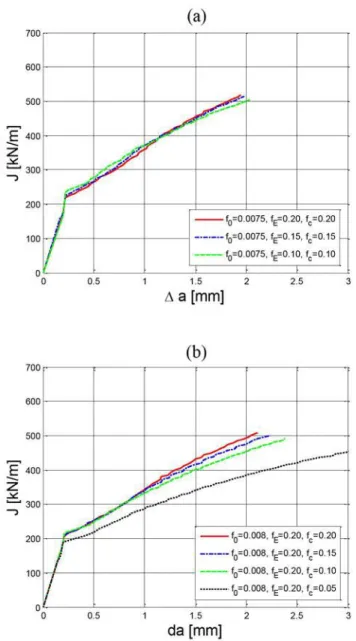
The parameters fcand fE, controlling the extinction of the cell element,

do not influence the JR- curve in any significant way if they are chosen

from the interval 0. 10 - 0.20, see Figure 2 . 3 . Values of fclower than 0.10

do however influence the JR- curve, see Figure 2 . 3 . Hence, the model

predictions are not sensitive to the choice of values for fcand fE, as long

as they are in the range 0.10 - 0.20.

Figure 2 . 3 . Comparison of numerical JR- curves for models with (a) varying fE

and fcvalues and (b) varying fcvalues.

(a)

12

The second step is to determine the fracture process parameters, this procedure is described in more detail in [3] . The fracture process parameters f0 and D are the main parameters controlling the crack

growth resistance behavior, in shear stress states with near zero triaxiality k also plays a significant role. To successfully determin e these parameters, experimental data describing the crack growth behavior and the behavior in pure shear is needed. An experimentally generated JR- curve is a suitable candidate for this purpose together with

results from a shear test. D can be determined from the crack tip opening displacement (CTOD) at initiation. CTOD scales with the near tip deformation and is also a relevant measure of the size of the fracture process zone. To take D as the CTOD at initiation is therefore suitable. CTOD at crack initia tion or D can be determined from JIc with the

relation

( 2. 7 )

where JIc is the J - value at initiation of crack growth, y is the yield

strength and d is a non - dimensional constant ranging from 0.30 to 0.60 depending on the material strai n hardening and yield strength [15] . The initial void volume fraction f0can be determined from matching the cell

model to the experimentally generated JR- curve. And finally, the shear

damage coefficient k is determined by matching the experimental results from a shear test to the predicted results from a FE - model. Below in Figure 2 . 4 the influence of f0on the JR- curve is illustrated and in

Figure 2 . 5 the influence of k on the predicted load deformation curve of a shear test is compared to experimental results.

Figure 2 . 4 . Effect of varying initial void volume fraction, f0, on the JR- curve,

13

Figure 2.5. Influence of values of kω on the predicted load deformation curve,

results from [6].

In order to generate a JR-curve from the numerical results of the cell model, the location of the crack front needs to be defined. In all analyses in this report, the crack front is defined by the line connecting locations at the crack plane where f=0.1. At f=0.1 a cell element has lost most of its load carrying capacity. Furthermore, the J-integral needs to be calculated. 0 1 2 3 4 5 6 0 1 2 3 4 5 6 Deformation [mm] Lo ad [kN ] FEM k_w=1.5 FEM k_w=1.7 Experimental results Experimental results

14

3.

Design of the Numerical

Experiments

To meet the goal of the project, to study the influence of residual stresses on fracture at low primary loads, ductile crack initiation and tearing is studied using models of test specimens. In these FE-models the ductile crack initiation and tearing is modelled using the cell model technique with a shear modified Gurson material model. The FE-models needed to be designed to give crack initiation at low primary loads and a well-defined residual stress field needed to be introduced. The first thing to decide during the design of the numerical experiments was how to introduce the residual stresses. The method with which the residual stresses are introduced will influence which type of fracture specimen that can be used. When the method of introduction of residual stresses and specimen type has been decided the size and material of the specimen can be decided. The size and material of the specimen governs at which Lr value crack initiation will occur. Two specimens were examined; one with, and one without, residual stresses. The numerical computations with the finite element method were executed with ABAQUS [12].

3.1.

_{INTRODUCTION OF RESIDUAL}

STRESSES

The residual stresses were introduced using the same method as in [2], [5] and [6], by a pre-load in compression of a notched specimen, see Figure 3.1. The pre-load leads to a stress concentration at the notch with compressive stresses normal to the crack surface. When the specimen is unloaded, a residual stress field is introduced due to the plastic deformations during the pre-load. The resulting residual stresses are tensile at the notch since they were compressive during the pre-load. This method to introduce the residual stress field gives a well-defined and predictable residual stress field without introducing unknown material changes and other uncertainties. For a more thorough description of the residual stress field and how it is introduced, see [2]. This method has earlier also been used successfully by other authors see the work by Mirzaee-Sisan et al. in [16].

15

Figure 3.1. In-plane compression of the notched test specimen.

The magnitude of the pre-load was determined such that the total strains in front of the crack tip did not exceed 1.5%. If the pre-load level is too high the material in front of the crack tip may be damaged due to high strains and the material would behave differently. The reason for the limit of 1.5% total strain is that no damage is introduced by pre-load levels below 1.5% of total strain in compression or tension, see results in Figure 3.2from earlier work in [5].

0 100 200 300 400 500 600 0 0.5 1 1.5 2 No pre-load No pre-load 1.5% comp 1.5% comp 3.0% comp 3.0% comp 6.0% comp 6.0% comp J [k N /m ] a [mm]

Figure 3.2. Effect from pre-load in compression on material fracture toughness, results from [5]. It can be seen that the specimens with no pre-load (black) are followed closely by 1.5 % strain specimens (blue).

Deviations in material behavoiur are observed from 3 % of total strains and up (green and red).

16

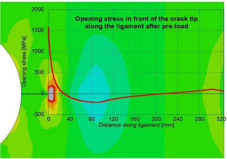
The size of the specimen also governs the pre - load magnitude. The size of the specimen is determined before calculating the pre - load magnitude , how the size is determined is described in Chapter 3.2 . When the size of the specimen had been set several FE - analyses were conducted resulting in a chosen pre - load of 17 M N. In Figure 3 . 3 the opening residual stress field in front of the crack tip created by the pre -load is shown.

Figure 3 . 3 . Opening residual stress field in front of the crack tip after pre -loading.

To correctly model the introduction of the residual stress field a separate FE - model was used. The reason for this was the exi s ting crack tip notch in the FE - model with cell elements , that introduces a stress concentration when the specimen is pre - loaded . This unwanted effect is however avoided if the crack tip is sharp . Therefore , a separate FE -model was used in obtaining a correct residual stress field. A n element layer was introduced at the crack surface during the pre - load, see Figure 3 . 4 , which was removed after unloading of the specimen.

Figure 3 . 4 . Introduced element layer during compressive pre - load.

17

The stress and strain results from the FE-model without cell elements (sharp crack-tip) were then used as pre-scribed initial conditions for the FE-model with cell elements (notched crack-tip).

3.2.

_{MATERIAL AND GEOMETRY}

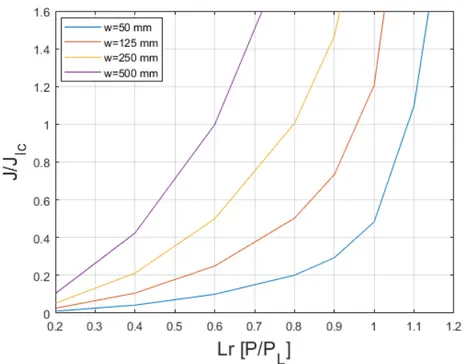
Next the material and the size of the specimen needed to be decided. The material was chosen to be A533B-1. The material properties of A533B-1 have earlier been thoroughly examined see [3], [5] and [6]. More information on the material and the material parameters for the shear modified Gurson model is given in Chapter 4.1.1. To determine the size of the specimen several FE-analyses were conducted. From these analyses predictions were made for the primary load at ductile crack initiation. Ductile crack initiation in these analyses was defined as JIc=200kN/m. In Figure 3.5 below some of the results from these predictions are shown.

Figure 3.5. Effect of specimen size on Lr value at ductile crack initiation for notched specimens without residual stress field.

From the results in Figure 3.5a specimen with W=500 mm was chosen. This would lead to ductile crack growth initiation at Lr=0.6 for

18

specimens without residual stresses according to the predictions. The geometry of the test specimen is shown in Figure 3 . 6 where W =500 mm.

Figure 3 . 6 . Base geometry of notched test specimen.

a R _L l1 S W

Geometry:

B =0.5 W

L =5 W

S =4 W

R =0.25

W

l1 =0.2 W

a =0.35

W

19

4. FE - modelling

4.1. FE - MODEL

A script was written by using the Python code language in order to create a parameterized FE - model for ABAQUS. With this script it is possible to model a 3PB specimen with a notch. The geometry of the test spe cimen is shown in Figure 3 . 6 where W =500 mm. With the script it is possible to control the cell element layer in great detail. During the course of the work several FE - mo dels were created with different setups of the element mesh. These were used in sensitivity analyses which led to the final element mesh setup described below. Due to symmetry, only a quarter of the test specimens were modelled. Figure 4 . 1 shows the FE - model used in the analyses.

Figure 4 . 1 . Three dimensional finite element mesh for a quarter model of an un - grooved notched three point bending specimen.

The fracture process zone or the cell element layer is shown in Figure 4 . 2 . The cell elements were model l ed with the height and length of D /2. The value of D and how it is determined is explained in Chapter 4.1.1 .

20

Figure 4 . 2 . The arrangement of the void containing cells (white elements) and the surrounding region.

The depth of the cell elements were varied with the position relative to the free surface with larger element de pths near the centre symmetry surface and with smaller depths near the free surface. At the free surface the element depth was equal to D /2. Both FE - models were meshed with a total of 20 element layers through the thickness. Figure 4 . 3 shows the element mesh trough the thickness. A thorough study of the influence of element thickness is presented by Qian in [17] and this study was decisive in de ciding the element layer setup. Both models used in the analyses were meshed with 8 - node linear brick element with reduced integration and hourglass control (C3D8R).

Figure 4 . 3 . The arrangement of the fin ite element meshes through the thickness used in the FE - model.

21

4.1.1.

_{MATERIAL MODEL PARAMETERS}

The material parameters for the shear modified Gurson model representing the A533B-1 ferritic steel have previously been determined in [6]. The same parameters were also used for the material model in the analyses presented in this report. The matrix material behaviour of the material model was modelled as elastic multi-linear plastic with isotropic hardening. The material parameters for the matrix material are given below in Table 4.1. The parameters in Table 4.1 were derived from uniaxial tensile test results presented in [6].

Table 4.1. Matrix material parameters used in the FE-model for material A533B-1. E = 205.3 GPa v= 0.3 σ [MPa] εpl 450.0 460.0 470.0 480.0 484.5 489.0 507.6 539.4 576.0 601.1 621.4 643.9 657.7 669.0 796.2 932.6 989.5 1050.0 0.0 0.00025 0.00119 0.00969 0.0130 0.0148 0.0185 0.0265 0.0384 0.0491 0.0603 0.0773 0.0911 0.1065 0.3681 0.7665 0.9912 1.9949

To be able to determine the micromechanical parameters q1 and q2 a power law curve is fitted to uniaxial tensile test results. The values for σ0 and N for the power law curve are then used to determine q1 and q2 from the tabulated values in [14]. The values of the void volume fractions fc and fE are typically chosen from the interval 0.10 to 0.20. The model predictions are rather insensitive to the choice of fc and fE as long as their values are in the interval mentioned above. In the following models fc and fE were set to 0.10 and 0.20 respectively. Table 4.2 below

22

presents the micromechanics parameters for the shear modified Gurson model.

Table 4.2. Micromechanics parameters used in the material model.

Micromechanics

q1 1.7046

q2 0.8503

fE 0.20

fc 0.10

The fracture process parameters f0 and D are the parameters primarily controlling the crack growth resistance behaviour. Hence, these are decided from an experimentally determined JR-curve using a standard specimen. The value of D was previously determined in [6] to 0.250 mm by using Equation 4 and the same value was used in the analyses presented in this report. The initial porosity f0 is determined by matching the cell model predictions to an experimental JR-curve. The value of the initial porosity f0 was set to 0.0070. The shear damage coefficient 𝑘𝜔 is determined by matching predicted FE-analyses results with experimental results. In [6] the value of 𝑘𝜔 was determined to 1.58 and this value was also used in the analyses presented in this report. Table 4.3 presents the fracture process parameters used in ABAQUS [12] for the shear modified Gurson model.

Table 4.3. Fracture process parameters used in the material model.

Fracture process

D [mm] 0.250 f0 0.0070

23

4.2.

CALCULATION OF THE J-INTEGRAL

To be able to interpret the results from the FE-models there was a need to calculate the J-integral. To calculate the J-integral a method using a correlation between Crack Mouth Opening Displacement (CMOD) and the integral was used. The correlation between CMOD and the J-integral was derived from several FE-analyses. To correctly evaluate the J-integral for the case with residual stresses the modified J-integral developed by Lei [18] was used. With this correlation the J-integral was obtained from the CMOD results. This method has previously been successfully used in [2], [5] and [6]. In Figure 4.4 an example of J-CMOD curves are shown.

Figure 4.4. Example of J-CMOD curves used in evaluating the J-integral from the numerical experiments.

Increasing crack depth

24

5.

Numerical Results

In Figure 5.1 the JR-curves generated by the numerical predictions for both FE-models are shown. The blue line corresponds to the model without a residual stress field and the red dashed line corresponds to the model with a residual stress field.

Figure 5.1. Predicted JR-curves for models with and without residual stress field.

As can be seen from the results in Figure 5.1 the residual stress field do not influence the material JR-curve. Hence, the material fracture toughness is not influenced by the residual stress field. This has also been seen earlier in the experimental work presented in [2]. In [2] crack initiation occurred at high primary loads. These results show that this is true even when you have crack initiation at low primary loads. This also reinforces the applicability of the modified J-integral [18] as a fracture mechanical parameter that can be used in predicting ductile crack growth initiation for cases with residual stresses.

In Figure 5.2 the predicted crack growth versus Lr (P/PL) for both models are shown. The blue line corresponds to the model without a residual stress field and the red dashed line corresponds to the model with a residual stress field. The crack growth initiation points are

25

marked with circles. It should be noted that the apparent growth seen before crack initiation is due to the blunting of the crack tip and also that the limit load (PL) for the specimen with initial crack depth is used in the definition of Lr. Hence, the limit load is held constant even after crack growth initiation.

Figure 5.2. Predicted crack growth versus Lr results for model with and

without residual stress field.

In Figure 5.3 the predicted J-values versus Lr (P/PL) are shown. The blue line corresponds to the model without a residual stress field and the red dashed line corresponds to the model with a residual stress field. As in Figure 5.2 the load is normalized by the limit load for the specimen with the initial crack depth.

26

Figure 5.3. Predicted J versus Lr results for model with and without residual

stress field.

The results in Figure 5.2 and Figure 5.3 clearly show an influence on crack initiation from the residual stress field. For the case without residual stresses the ductile crack initiation occurred at Lr=0.60 while with residual stress field crack initiation occurred at Lr=0.31. Hence, a residual stress field have a significant effect on ductile crack initiation at low primary loads. It should be noted that our pre-analysis predictions was to get initiation at Lr=0.60 for the specimen without residual stress field see Figure 3.5. If 2 mm stable crack growth is considered it can also be seen that the residual stress field have an influence. For the model without residual stress field a ductile crack growth of 2 mm corresponds to Lr=0.89 and for the model with residual stress field Lr=0.70. Hence, even with a limited amount of ductile crack growth the influence from the residual stresses is still present.

Crack initiation

2 mm ductile crack growth

27

Figure 5.4. Relative difference in predicted J values for model with and without residual stress field

In Figure 5.4 above the relative difference for predicted J results from the model with and without residual stress field is shown. Here it can clearly be seen that the relative difference decreases as the primary load increases. The decrease of influence from the residual stresses is not due to ductile crack growth, instead it is due to an increased primary load that gets closer to the limit load. This conclusion is strengthened by the experimental results presented in [2] where the same behaviour is seen but for those cases the initiation occurred at Lr=1.1. Hence for those cases there are no ductile crack growth and the only influencing factor is an increased primary load that gets closer to the limit load. It should also be noted that the results presented above do not contradict the analysis strategy presented in [1] which suggests a reduction of the safety factor for residual stresses at primary loads above Lr=0.8.

28

6.

Comparison between numerical

predictions and predictions made

using R6

In Sweden the nuclear industry mainly uses the procedure described [19] for assessment of cracks or crack like defects and for defect tolerance analysis. This procedure is based on the R6-method [20]. Therefore, it is of interest to investigate the inbuilt conservatism in the R6-method [20]. The results obtained from the numerical predictions are compared with results calculated using the R6 procedure to evaluate the conservatism of the R6 method. The approximate option 2 curve described in the R6-method, revision 4 [20] and the simplified method without the ρ-factor are used to calculate the J-integral.

6.1.

CALCULATING THE J-INTEGRAL

USING R6

Calculating the J-integral using the R6-method uses the R6 function with the elastic solution of KI to get an approximate elastic-plastic J solution as given in Equation 6.1. In the R6-method, the linear elastic stress intensity factor KI is divided in two parts; one part from the secondary stresses 𝐾_𝐼𝑆 _{and one part from the primary stresses 𝐾}

𝐼𝑃. When secondary stresses are present, the ρ-factor or alternatively the factor V is also used in the calculations. In Sweden the Nuclear industry uses a procedure described in [19] for assessments of defects. The procedure described in [19] use the R6-method and the factor. Therefore, the ρ-factor is used in all the calculations performed within this report. It should be mentioned that the ρ-factor is not present in the latest revision of the method [20] it has been replaced by the factor V. In the R6-method revision-4 [20] a more detailed description of the J-estimation approach is given using the factor V in [19] more information about the ρ-factor is given. Below is a short description of how the J-integral is estimated according to the R6-method using the ρ-factor.

𝐽(𝐿_𝑟) = (𝐾𝐼𝑃+𝐾𝐼𝑆) 2

𝐸′_[𝑓(𝐿

𝑟)−𝜌]2 (6.1)

𝐾_𝐼𝑃 is the linear elastic stress intensity factor derived from the primary load depending on Lr, 𝐾_𝐼𝑆 is the linear elastic stress intensity factor from the secondary stresses, f(Lr) is the failure assessment curve in the R6-method, ρ is a correction factor depending on Lr, and E´ is the effective elastic modulus as defined below:

29 𝐸 ´ = {

𝐸

1−𝑣2, for plane strain condition

𝐸, for plane stress condition (6.2)

The approximate option 2 curve f2(Lr) from R6 revision 4 is used when estimating the J results. The option 2 curve is also used in the procedure described in [19]. The approximate option 2 curve f2(Lr) from R6 revision 4 is material dependent. Further the ρ-factor is evaluated using the following expression,

𝜌 = 𝜓 − 𝜑(𝐾𝐼𝑆

𝐾_𝐽𝑆− 1), (6.3)

30

6.2.

_{COMPARISON BETWEEN NUMERICAL}

PREDICTIONS AND R6 PREDICTIONS

Below in Figure 6.1 and Figure 6.2 the results from the comparison using the approximate option 2 curve with the ρ-factor are shown.

Figure 6.1. Comparison between numerically predicted J and J estimated using R6 approximate option 2 curve with the ρ-factor for the case with and without residual stress field.

Figure 6.2. J estimated using R6 approximate option 2 curve normalized with numerical predicted J values.

31

The results presented in Figure 6.1 and Figure 6.2 show that for the case without residual stress field the R6 approximate option 2 curve give very good estimates of the J-integral. But for the case with residual stress field the R6 estimation of the J-integral is conservative. These results are similar and matches earlier results presented in [21]. The results presented in [21] where for cases where crack initiation occurred at high primary loads in the results presented in this report crack initiation occurs at low primary loads. Hence estimation of the J-integral using the R6 approximate option 2 curve with the ρ-factor can be said to give conservative estimates of the J-integral irrespective of primary load level at crack initiation.

Below in Figure 6.3 and Figure 6.4 the results from the comparison using the approximate option 2 curve without the ρ-factor are shown.

Figure 6.3. Comparison between numerically predicted J and J estimated using R6 approximate option 2 curve without the _{ρ-factor for case with and} without residual stress field.

32

Figure 6.4. J estimated using R6 approximate option 2 curve without the ρ-factor normalized with numerical predicted J values.

The results presented above show that for the case with and without residual stress field the R6 approximate option 2 curve without the ρ-factor give very accurate estimates of J for geometries used within this report.

33

7.

Discussion

From the presented results a lowering of the safety factor for secondary stresses at low primary loads (Lr<0.8) cannot be recommended. The results do not contradict the conclusions from earlier [3] studies that lowering of the safety factor for secondary stresses at high primary loads (Lr>0.8) according to the procedure described in [2] is a sound approach.

The results do not show any diminishing effects on the crack driving force from the residual stresses due to ductile crack growth. Hence, a lowering of the safety factor for secondary stresses in cases where 2 mm stable crack growth is considered is not recommended.

On the other hand, the results demonstrate the validity to use the modified J-integral as a fracture mechanical parameter to predict ductile crack growth initiation for cases with residual stresses. This leads to a possibility to reduce conservatism in the R6 method by performing more detailed analysis. By using the modified J-integral in assessing defect in the presence of a residual stress field the inbuilt conservatism in the R6 method can be avoided. An alternative approach is to use the R6 procedure without the ρ-factor but calculating the contribution from the residual stresses (Jres) with FE-analyses using the modified J-integral. As can be seen in Figure 6.4 this approach also reduces the inbuilt conservatism generated by the ρ-factor in the R6 method for geometries used within this report. Furthere studies are needed to confirm if this is also true for an arbitrary geometry.

In ASME XI Code Case N-749 [22] it is suggested that the same safety factors as in Appendix C could be used for a reactor pressure vessel steel in the “upper shelf region”. In code case N-749 they also argue that the residual stresses do not need to be included in flaw assessment when using proposed code case N-749. The argument for not including the residual stresses in flaw assessments seems to be based on assumptions that would be correct regarding the failure at high primary loads near or above the limit load (Lr≥1) or due to plastic collapse. All the reported fracture tests that are referred to in code case N-749 argumentation have experienced ductile initiation at primary loads near or above the limit load (Lr≥1) where the influence of the residual stresses are negligible. The referred fracture tests do not give any information of the influence from residual stresses on ductile fracture at low primary loads (Lr<0.8). Hence the argumentation for not including residual stresses in flaw assessments in code case N-749 is inconclusive. Furthermore, it could be argued that the recommendation to not include residual stresses is even erroneous as we have shown in this report that the influence from the residual stresses are not negligible at low primary loads (Lr<0.8) even when we consider some ductile crack growth. Therefore, it is recommended to not adapt code case N-749.

34

8.

Conclusion

All the conclusions are valid for an arbitrary residual stress field and for ferritic materials in the upper shelf regime. From the results presented in this report the following conclusions can be drawn:

 Residual stresses do not influence the material fracture toughness.

 Residual stresses have an effect on crack initiation at low primary loads Lr<0.8.

 The effect of residual stresses on ductile fracture does not decrease with limited ductile crack growth, the driving force from the residual stresses persists.

 The effect from residual stresses do diminish at high primary loads near and above Lr=1, due to extensive plasticity.

 The modified J-integral as a fracture mechanical parameter can be used in predicting ductile crack growth initiation for cases with residual stresses.

 The R6 procedure with the use of ρ-factor gives conservative estimates of the J-integral for geometries used within this report.  The R6 procedure without using the ρ-factor gives very accurate

estimates of J-integral when calculating the Jres using elastic-plastic FE-analysis and the modified J-integral for geometries used within this report.

35

9.

References

[1] P. Dillström, M. Andersson, I. Sattari-Far and W. Zhang, "Analysis strategy for fracture assessment of defects in ductile material," Strålsäkerhetsmyndigheten, Report number: 2009:27, 2009.

[2] T. Bolinder and I. Sattari-Far, "Experimental evaluation of influence from residual stresses on crack initiation and ductile crack growth at high primary loads," Strålsäkerhetsmyndigheten, Report number: 2011:19, 2011.

[3] X. Gao, J. Faleskog and C. Shih, "Cell model for nonlinear fracture analysis – II. Fracture-process calibration and verification," International Journal of Fracture, vol. 89, pp. 375-398, 1998.

[4] X. Gao, J. Faleskog and C. Shih, "Ductile tearing in part-through cracks: experiments and cell model predictions," Engineering Fracture Mechanics, vol. 59, no. 6, pp. 761-777.

[5] T. Bolinder, "Numerical simulation of ductile crack growth in residual stress fields," Strålsäkerhetsmyndigheten, Report number: 2014:28, 2014.

[6] T. Bolinder, "Ductile tearing – Micromechanical analyses and experimental study," Strålsäkerhetsmyndigheten, Report number: 2015:53, 2015.

[7] K. Nahshon and J. Hutchinson, "Modification of the Gurson Model for shear failure," European Journal of Mechanics A/Solids, vol. 27, pp. 1-17, 2008.

[8] L. Xia and C. Shih, "Ductile crack growth - I. A numerical study using coputational cells with a microstructurally-based length scale," Journal of the Mechanics and Physics of Solids, vol. 43, pp. 233-259, 1995.

[9] L. Xia and C. Shih, "Ductile crack growth - II. Void nucleation and geometry effects on microscopic fracture behavior," Journal of the Mechanics and Physics of Solids, vol. 43, pp. 1953-1981, 1995.

[10] A. Gurson, "Continuum theory of ductile rupture by void nucleation an growth: Part I – Yield criteria and flow rules for porous ductile media," Journal of Engineering Materials and Technology, vol. 99, pp. 2-15, 1977.

[11] V. Tvergaard, "Material failure by void growth to coalescence," Advances in applied Mechanics, no. 27, pp. 83-151, 1990. [12] Hibbit, Karlsson and Sorenson, ABAQUS user manual, Dassault

Systèmes.

[13] V. Tvergaard and A. Needleman, "Analysis of cup-cone fracture in a round tensile bar.," Acta Metallurgica, vol. 32, pp. 157-169, 1984.

36

[14] J. Faleskog, X. Gao and C. Shih, "Cell model for nonlinear fracture analysis – I. Micromechanics calibration," International Journal of Fracture, vol. 89, pp. 355-373, 1998.

[15] C. Shih, "Relationship between the J-integral and the crack opening displacement for stationary and extending cracks," Journal of the Mechanics and Physics of Solids, vol. 29, pp. 305-326, 1981.

[16] A. Mirzaee-Sisan, C. E. Truman, D. J. Smith and M. C. Smith, "Interaction of residual stress with mechanical loading in ferritic steel," Engineering Fracture Mechanics, vol. 74, pp. 2864-2880, 2007.

[17] X. Qian, "An out-of-plane length scale for ductile crack extensions in 3-D SSY model for X65 pipeline materials," International Journal of Fracture, vol. 167, pp. 249-265, 2011. [18] L. Y., "J-integral evaluation for cases involving

non-proportional stressing.," Engineering Fracture Mechanics, vol. 72, pp. 577-596, 2005.

[19] P. Dillström, J. Gunnars, P. von Unge and D. Mångård,

"Procedure for Safety Assessment of Components with Defects," Strålsäkerhetsmyndigheten, Report number: 2018:18, 2018. [20] R6, Assesment of the integrety of structures containing defects,

Revision 4, EDF Energy Nuclear generatiom Ltd, 2015. [21] T. Bolinder and J. Faleskog, "Evaluation of the Influence of

Residual Stresses on Ductile Fracture," Journal of Pressure Vessel Technology, vol. 137, 2015.

[22] H. L. Gustin, R. C. Cipolla, S. X. Xu and D. A. Scarth, "Alternative acceptance criteria for flaws in ferritic steel components operating in the upper shelf temperature range," in Proceedings of the ASME 2012 Pressure Vessels & Piping Conference, PVP2012, Toronto, Canada, 2012.

Strålsäkerhetsmyndigheten Swedish Radiation Safety Authority

SE-171 16 Stockholm Tel: +46 8 799 40 00 E-mail: registrator@ssm.se

Web: stralsakerhetsmyndigheten.se

2019:27 The Swedish Radiation Safety Authority has a comprehensive responsibility to ensure that society is safe from the effects of radiation. The Authority works to achieve radiation safety in a number of areas: nuclear power, medical care as well as commercial products and

services. The Authority also works to achieve protection from natural radiation and to increase the level of radiation safety internationally.

The Swedish Radiation Safety Authority works proactively and preventively to protect people and the environment from the harmful effects of radiation, now and in the future. The Authority issues regulations and supervises compliance, while also supporting research, providing training and information, and issuing advice. Often, activities involving radiation require licences issued by the Authority. The Swedish Radiation Safety Authority maintains emergency preparedness around the clock with the aim of limiting the aftermath of radiation accidents and the unintentional spreading of radioactive substances. The Authority participates in international co-operation in order to promote radiation safety and finances projects aiming to raise the level of radiation safety in certain Eastern European countries.

The Authority reports to the Ministry of the Environment and has around 300 employees with competencies in the fields of engineering, natural and behavioural sciences, law, economics and communications. We have received quality, environmental and working environment certification.

Ale

Tryckteam