Research
2010:12
An Evaluation of Models of
Bentonite Pore Water Evolution
Authors: David SavageRandy Arthur Claire Watson James Wilson
Title: An Evaluation of Models of Bentonite Pore Water Evolution Report number: 2010:12
Author: David Savage1, Randy Arthur2, Claire Watson1 and James Wilson1 1.Quintessa Ltd, The Hub, 14 Station Road, Henley-on-Thames, RG91AY, UK
2.Monitor Scientific LLC, 3900 south Wadsworth Boulevard, Denver, Colorado 80235, USA
Date: Januari 2010
This report concerns a study which has been conducted for the Swedish Radiation Safety Authority, SSM. The conclusions and viewpoints presented in the report are those of the author/authors and do not necessarily coin-cide with those of the SSM.
SSM Perspective
Background
The pore-water composition of a KBS-3 bentonite buffer may gradually change as a result of reaction between groundwater and buffer minerals. The rather minor occurrences of the most rapidly reacting minerals in the buffer will have the most immediate and observable influences, but contributions from slow reactions of the main bulk clay phases cannot be ruled out. The performance implication of such bentonite chemical reaction is that radionuclide solubility and sorption depend on the buffer chemical conditions. Moreover, pore-fluid composition at the interface between the buffer and the surrounding bedrock is important for the modelling and assessment of potential buffer loss scenarios. Any process with the potential to affect this composition needs to be identi-fied and analysed.
Purpose of the Project
The purpose of this project is to assess to smectite hydrolysis as a poten-tial contribution to long-term geochemical processes in a KBS-3 bento-nite buffer.
Results
The outcome of this project is a suggested modelling approach for handling the influences of smectite clay transformations in the perfor-mance evaluation of a KBS-3 bentonite buffer. In the more traditional buffer geochemical modelling approach, the focus has been on more reactive trace constituents such as calcite, gypsum and pyrite, but the potential bulk-transformation of the main constituent cannot be igno-red without justification. In absolute quantitative terms, several uncer-tainties remain, such as the validity of thermodynamic estimates for smectite properties, the validity of the buffer porosity model, the influ-ence of reaction kinetics and the nature of precipitating new minerals. It is concluded in this study that smectite hydrolysis may (based on model predictions) be significant for the future geochemical state of a buffer, but that the time-scale of smectite hydrolysis is too long for experi-mental verification. The utilized experiexperi-mental data could therefore not
determine whether or not the process has performance implications for safety assessment. Potential performance significances of such process are as described above related to buffer pH variations and pore-fluid cation composition.
Future work
The authors suggest that the importance of smectite hydrolysis could be further studied through field observation of natural clay-water systems that have evolved over long time scales. Additional exploratory geoche-mical or bounding performance calculations could also be envisaged. The groundwater evolutionary pathway at potential repository sites with consideration of other engineering materials such as cement could be analysed with the purpose of determining thermodynamic driving forces for smectite alteration.
Project Information
Project manager: Bo Strömberg Project reference: SSM 2008
Content
1. Introduction ...5
2. Conceptual Models for Clay Pore Fluid Behaviour...7
3. Experimental Data ...11
4. Model Input...15
4.1 Bentonite compositions...15
4.2 Ion exchange and surface reactions ...15
4.3 Mineral hydrolysis ...15
4.3.1 Smectite...15
Estimation using the Vieillard model...17
Estimation using the Polymer model ...19
4.3.2 Other minerals, secondary minerals and aqueous species .21 4.4 Kinetics ...21
4.4.1 Smectite...21
4.4.2 Other minerals in bentonite and secondary minerals...23
4.5 Pore water compositions ...23
5. Model results...25
5.1 Scoping calculations ...25
5.2 Consideration of reaction kinetics...27
5.3 Time- and space-dependent calculations ...34
5.3.1 Case D – smectite hydrolysis only ...36
5.3.2 Cases E1 and E2 – inclusion of secondary mineral growth.36 5.3.3 Case F – geochemical porosity model ...36
5.3.4 Cases G1 and G2 – inclusion of ion exchange ...39
5.3.5 Case J – increased reservoir mixing length ...41
5.3.6 Case M – alternative kinetic model for smectite...42
5.3.7 Case N – inclusion of CO2(aq)...42
5.3.8 Case Q – reduction of diffusion coefficient...42
5.3.9 Case R – exclusion of ion exchange ...45
6. Conclusions ...47
Executive Summary
The determination of a bentonite pore water composition and understanding its evolution of with time underpins many radioactive waste disposal issues, such as buffer erosion, canister corrosion, and radionuclide solubility, sorp-tion, and diffusion, inter alia.
The usual approach to modelling clay pore fluids is based primarily around assumed chemical equilibrium between Na+, K+, Ca2+, and Mg2+ aqueous species and ion exchange sites on montmorillonite, but also includes proto-nation-deprotonation of clay edge surface sites, and dissolution-precipitation of the trace mineral constituents, calcite and gypsum. An essential feature of this modelling approach is that clay hydrolysis reactions (i.e. dissolution of the aluminosilicate octahedral and tetrahedral sheets of montmorillonite) are ignored. A consequence of the omission of clay hydrolysis reactions from bentonite pore fluid models is that montmorillonite is preserved indefinitely in the near-field system, even over million-year timescales.
Here, we investigate the applicability of an alternative clay pore fluid model, one that incorporates clay hydrolysis reactions as an integral component and test it against well-characterised laboratory experimental data, where key geochemical parameters, Eh and pH, have been measured directly in pacted bentonite. Simulations have been conducted using a range of com-puter codes to test the applicability of this alternative model. Thermody-namic data for MX-80 smectite used in the calculations were estimated using two different methods.
Simulations of ‘end-point’ pH measurements in batch bentonite-water slurry experiments showed different pH values according to the complexity of the system studied. The most complete system investigated revealed pH values were a strong function of partial pressure of carbon dioxide, with pH increas-ing with decreasincreas-ing PCO2 (log PCO2 values ranging from -3.5 to -7.5 bars
produced pH values ranging from 7.9 to 9.6).
A second set of calculations investigated disequilibrium between clay and pore fluid in laboratory squeezing cell tests involving pure water (pH = 9.0) or a 1M NaOH solution (pH = 12.1). Simulations carried out for 100 days (the same timescale as the experiments) showed that smectite remained far from equilibrium throughout, and that pH decreases due to smectite hydroly-sis were trivial. However, extending the duration of the simulations to that required for clay-fluid equilibrium, necessitated timescales of 7 and 65 years for pure water and 1M NaOH, respectively, but again produced relatively minor pH decreases in the order of 0.1-0.2 pH units. If the (equilibrium) precipitation of secondary minerals was included in the simulations, then not only was the clay-fluid equilibration period extended dramatically (from 7 to 360 years for pure water, and from 65 to 2600 years for 1 M NaOH), but concomitant changes in pH were significant, decreasing from 9.0 to 8.6 (pure water) and from 12.1 to 9.0 (1 M NaOH). Repetition of these latter calculations using an alternative method of estimating the ΔGf
0
produced an increase in equilibration time for reaction with 1M NaOH from 2600 to 5000 years, highlighting the potential effects of the uncertainty in thermodynamic data for smectite.
A final set of calculations was carried out to investigate both the time- and space-dependent variations in pore fluid composition in laboratory in-diffusion experiments conducted for over 1200 days, initially with pure wa-ter and ‘spiked’ afwa-ter 271 days with a Na-Ca-OH-Cl solution (pH = 11.7). Here, the sensitivity of the results to both variations in a number of parame-ters/conditions (porosity, reaction rate of secondary minerals, the degree of mixing of the external fluid reservoirs in the experiments, the effective diffu-sion coefficient) and the includiffu-sion/excludiffu-sion of key processes (clay hydroly-sis, secondary mineral precipitation, ion exchange, clay edge protonation-deprotonation reactions) was investigated. These calculations confirmed that smectite hydrolysis alone has an insignificant impact upon pH buffering over lab timescales and that the pH buffering observed is most likely con-trolled by clay protonation-deprotonation reactions, and kinetic secondary mineral (brucite + tobermorite) precipitation, using a total porosity model (simulations using a geochemical porosity value produced a poor fit to the experimental data). Ion exchange was not important in controlling pH. The pH of the initial bentonite pore water is ascribed to the presence of trace amounts of CO2 in the experiments, although calcite played an insignificant
role in pH buffering. Alternative data for the kinetic hydrolysis of smectite produced no observable differences, and the adoption of a reduced diffusion coefficient produced a poorer fit to experiment results.
In conclusion, modelling predicts that the effects of smectite dissolution on the chemistry of bentonite pore waters would be essentially undetectable over experimental time scales, but when the model is combined with plausi-ble constraints on the precipitation of secondary phases, significant changes in solution chemistry and mineralogy are predicted to occur over time scales that are relevant to repository near-field evolution (hundreds to thousands of years). There are remaining fundamental uncertainties related to the variable chemistry of the smectite clays, the nature of porosity in highly compacted buffer materials, the reactive surface area of smectite, and the thermody-namic properties of these clay minerals. Studies of natural clay-water sys-tems that have evolved over long periods of time could help provide a new perspective on these uncertainties, and approaches that could be used to help resolve them.
1. Introduction
The determination of a bentonite pore water composition and understanding the evolution of its likely chemical composition with time underpins many other repository near-field activities, such as understanding buffer erosion, canister corrosion, and radionuclide solubility, sorption, and diffusion, inter alia and thus plays a vital, if indirect, rôle in safety assessment.
Key parameters in definition of this pore water composition are pH and Eh, which have major effects on canister corrosion and radionuclide solubility and migration, and concentrations (activities) of aqueous species which may accelerate metal corrosion, and/or enhance radionuclide
solubili-ties/mobilities. Species in this category would include HS-, HCO3
-, and Cl-. An important aspect of this evaluation is not only to define a (starting) pore water composition, but also to gain insight into controlling processes and mechanisms, such that changes in pore water composition can be predicted when the system is subject to internal (e.g. waste thermal output) and exter-nal (e.g. changing host rock groundwater composition) perturbations. Redox in bentonite pore fluids is generally assumed to be controlled by chemical equilibria involving dissolved iron species and iron-bearing miner-als, such as Fe2+/Fe3O4 (e.g. [1]), or alternatively, by Fe
2+
/siderite (e.g. [2]). Reactions involving reduced sulphur species are deemed of lesser impor-tance because of the assumed non-viability of sulphate-reducing bacteria in compacted bentonite ([2]). To a certain extent, the precise controlling reac-tions are a site-specific issue, in that the concentrareac-tions of redox-sensitive species may be dominated by the composition of the ambient groundwater at a disposal site.
pH is assumed to be determined through the interaction of a number of fac-tors, such as:
ion exchange on clay;
protonation-deprotonation reactions at clay edge sites;
dissolution-precipitation reactions of trace carbonate minerals (cal-cite, siderite, dolomite);
dissolution-precipitation reactions of the major clay mineral compo-nent (montmorillonite) of the bentonite;
the concentration of conservative anions (usually Cl-) in the ambient groundwater;
and the assumed partial pressure of carbon dioxide (PCO2) of the
system.
Different authors place different emphasis on each of the above factors, but the consensus is that the clay fraction principally acts as a cation exchanger, with the clay silicate exchanger being essentially inert and pH being deter-mined by the contribution from the trace carbonate mineral concentration, and the ambient PCO2/chloride activity (e.g. [2]; [1]). However, there are
question marks concerning the thermodynamic validity of ion exchange-based models for clay (e.g. [3]), and a more rigorous approach employing a
solid-solution model for montmorillonite has been advocated ([4]). Ironi-cally, the corollary of this is that although bentonite is part of the ‘engi-neered’ barrier system, to all intents and purposes, adoption of an ion ex-change-based model necessitates that pH is fixed by the ambient geochemi-cal conditions (PCO2, [Cl-]) at a repository location, rather than by the
essen-tial mineral component (montmorillonite) of the bentonite itself.
A consequence of the omission of clay hydrolysis reactions from pore fluid evolution models is that montmorillonite is preserved indefinitely in the near-field system, even over million-year timescales. However, this is con-trary to natural systems evidence where smectite clays may undergo dissolu-tion-precipitation reactions over assessment-relevant timescales at pH 9-10 and temperatures of 50-60 °C (e.g. [5]). It may be concluded therefore that although the current approach may be satisfactory to interpret the results of laboratory or in situ experiments, it is not necessarily sufficient to be ex-tended to the timescales of interest for repository safety assessment. Here, we propose an alternative clay pore fluid model, one which incorpo-rates clay hydrolysis reactions as an integral component of the model and is tested against suitable well-characterised laboratory experimental data. Re-searchers at VTT in Finland have reported the results of laboratory experi-ments which have measured key geochemical parameters, Eh and pH, di-rectly in compacted bentonite ([6]). These measurements have been achieved by using solid-state electrodes in conjunction with standard chemi-cal analysis of squeezed pore fluids for chemi-calibration purposes. Experiments have been conducted in diffusion cells, squeezing cells, and batch type appa-ratus, thus providing both single ‘end-point’ type results and time- and space-dependent squeezing and in-diffusion results. Data from these experi-ments provide a means of testing geochemical models for bentonite pore fluid evolution and have provided the focus for the modelling activities de-scribed here.
2. Conceptual Models for
Clay Pore Fluid
Behav-iour
Intimately related to any model of the evolution pore fluid composition is the understanding of pore fluid behaviour in compacted bentonite, particularly with regard to the nature of porosity and the behaviour of fluids in close proximity to charged clay surfaces. Currently-available conceptual models for clay-pore fluid behaviour consist of either a system with different poros-ity types, or a system with a single porosporos-ity. Both models are discussed in more detail below.
Many researchers view compacted bentonite as possessing different types of porosity, (e.g. [7]; [8]; [9]; [10]; [11]; [6]; [12]) (Figure 1). In this concept, ‘total porosity’ refers to the total volume of voidage, without discrimination regarding location or type, whereas ‘interlamellar/interlayer porosity’ is lo-cated in the interlayer spaces of individual clay particles, between the indi-vidual tetrahedral-octahedral-tetrahedral (TOT) sheets ([10]). This is con-sidered to be a few monolayers thick and because of its more structured na-ture, is likely to have different properties from ‘free water’. ‘External poros-ity’ can be viewed as being of two types: that which consists of water in electrical double layers on the surfaces of the clay particles (‘double layer water’); ‘free water’ ([10]) or ‘chloride porosity’ ([6]), which consists of water as interconnected thin films on the outside of clay stacks and also as films surrounding other minerals (e.g. quartz) in the bentonite. The amounts of each porosity type are thought to vary with compaction density in ben-tonite (e.g. [13]), with free/chloride porosity being significantly less than the total porosity as compaction density increases (Figure 2).
In this model, diffusion of cations is envisaged to take place both through the interlamellar porosity and the free porosity, whereas diffusion of chloride and other anions takes place solely though the free porosity (e.g. [12]). At high ionic strengths, diffusion of cations is thought to take place preferen-tially though the free porosity. This interpretation leads to an effective diffu-sion coefficient which varies according to ionic strength. A corollary of this conceptual model is that bentonite acts as a semi-permeable membrane at high compaction densities, and is effectively impermeable to ionic species in groundwater external to the bentonite ([9]). However, this is contrary to some experimental evidence where ‘external ions’ have been shown to be introduced to bentonite at high compaction densities (e.g. [14]).
Figure 1. Schematic diagram of the nature of water in compacted bentonite. From [10].
Figure 2. Different porosity types in compacted bentonite. 1 = total poros-ity; 2 = external porosity (‘double layer’ water + ‘free’ water); 3 = ‘inter-lamellar’/’interlayer’ porosity; 4 = ‘chloride’/’free’ porosity; 5 = porosity inaccessible by chloride. From [13].
An alternative conceptual model to that described above is offered by Karnland and co-workers ([14]; [15]) which consists of a bentonite-pore fluid system consisting of one porosity type and where pore fluid composi-tion is controlled by ion equilibria within the interlamellar pore space involv-ing two basic processes: Donnan equilibrium which reduces concentrations of external ions compared with external pore fluids; and cation exchange, which affects systems only with more than one type of cation. Conse-quently, the clay-pore fluid system is envisaged to consist of clay particles acting as macro-ions, and the entire clay-water system may be viewed as a ‘polyelectrolyte’ (Figure 3).
Birgersson and Karnland ([15]) derive a general expression to describe the effective diffusion coefficient (De) for transport of aqueous species in com-pacted bentonite:
Dec
2 Dc (1)
where c is the total clay porosity; is a general ion equilibrium coefficient;
ς describes the influence of filters (in experimental systems with filters sepa-rating fluid reservoirs from the clay), and Dc is the diffusion coefficient in
the clay. Normally (for typical filters and sample lengths), the parameter ς is only of importance for cation tracers in very low background concentrations, since the flux of the tracer then will be very high and the filters may be a restriction (O. Karnland, pers. comm.). The ion equilibrium coefficient (Ξ) is a general coefficient in order to express the concentration discontinuities over the solution/bentonite interface. In the case of anions, Ξ represents the Donnan equilibrium effect, whereas in the case of cations, Ξ represents the combined effects of cation exchange and Donnan equilibrium. At low and medium background concentrations, only the ion exchange term is of impor-tance (O. Karnland, pers. comm.). The typical situation for tracer tests in bentonite is that anion concentration will be strongly suppressed in the ben-tonite, and that cation concentrations will be strongly enhanced.
Birgersson and Karnland ([15]) argue that the acceptance of the existence of only one type of porosity in compacted bentonite obviates the need to de-scribe two separate methods of describing anion and cation diffusion and thus their model brings a greater symmetry to the understanding of transport in compacted bentonite. Thus removing all but one type of pore structure greatly reduces the amount of model parameters to one, the interlayer pore diffusivity (Dc). Furthermore, the single pore type model is not only
consis-tent with, but also allows for calculation of, the swelling pressure under various physicochemical conditions ([16]; [17]).
+
+
+
+
+
+
+
+
+
-
--
--
-+
+
+
+
+
electrolyte clay introduced ionsFigure 3. The single porosity model of the clay-pore fluid system. The clay is seen as a ‘soluble polyelectrolyte’, contributing positively and negatively charged ions to the clay-water system. An osmotic equilibrium is set up between the clay and external electrolyte, involving diffusion of water mole-cules and ionic species. From [18].
The findings of Birgersson and Karnland ([15]) also have large implications for the conceptual view of pore water chemistry. Since in their model, the major part of cations and anions reside in the interlayer pores, this volume is of crucial importance and cannot be ignored in characterising the bentonite pore water chemistry. This approach is thus in sharp contrast to the ‘variable porosity’ model where pore fluid is considered to reside in the ‘free water’ porosity only.
3. Experimental Data
VTT in Finland has reported laboratory experimental data concerning the in situ measurement of Eh and pH in compacted bentonite ([6]; [19]). It is considered that these data currently constitute the best test of the accuracy of bentonite pore fluid models over short timescales. VTT conducted three basic types of experiments: ‘batch’; ‘squeezing’; and ‘diffusion’. The batch and squeezing experiments were similar in that both resulted in single ‘end-point’ calculations of pH. The diffusion experiments modelled the evolution of pH (and Eh in some instances) over long timescales (in excess of 1200 days).
Muurinen and Carlsson ([6], [19]) carried out 3 batch experiments in centri-fuge tubes. These experiments employed lower bentonite densities than squeezing experiments (below) and fluids were separated at the end of each experiment by centrifugation. Experiment durations were 12 days. Ben-tonite densities, porosities (total, and what Muurinen and Carlsson ([6], [19]) describe as ‘external’ and ‘chloride’ porosities) and pH were all meas-ured/calculated.
Muurinen and Carlsson ([6], [19]) also carried out three experiments in squeezing apparatus. The initial bentonite dry density was about 8 %. These experiments contained approximately 11 g of clay and approximately 9 g of (pure) water. The experiments were conducted for 21 days. Again, ben-tonite densities, porosities (total, and what Muurinen and Carlsson ([6], [19]) describe as ‘external’ and ‘chloride’ porosities) and pH values were meas-ured. The results of all pH measurements in experiments ‘L1’ and ‘L2’ are shown in Figure 4 and Figure 5, respectively.
Muurinen and Carlsson ([6], [19]) describe an experiment in a cylindrical diffusion cell (‘experiment DIF6’) in which they monitor pH in compacted bentonite, both before and after, introduction of a high pH, high salinity fluid (Figure 6). In these experiments, bentonite was mixed with deionised water and compacted, before transferral to a diffusion cell. The bentonite sample had a target dry density of 1.5 g cm-3, with a diameter of 40 mm and length of 50 mm. The total porosity was nominally 45.6 % and the geochemical (free) porosity was 6 %. The bentonite remained in contact with an external solution of 10 ml volume via a titanium filter plate. The bentonite sample cell had measurement electrodes at 5, 10, and 20 mm from the contact with the external solution. The apparatus was kept in a nitrogen-filled glovebox for the duration of the experiment. The total duration of the experiment was in excess of 1200 days. The measured in situ pH at various depths within the clay sample versus time in the diffusion experiment is presented in Figure 7.
Figure 4. Summary of pH measurements in experiment L1 ([6], [19]). The composition of the final squeezed porewater (pH 9) is shown in Table 8. Initial in-situ measurements using the IrOx electrode (‘in bentonite’) are
affected by transient disturbances to the bentonite-water system caused by emplacement of the reference electrode ([6], [19]). These disturbances largely dissipate within a day or two.
Figure 5. Summary of pH measurements in experiment L2 ([6], [19]). The composition of the final squeezed pore water (pH 12.1) is shown in Table 8.
Measurements using the IrOx electrode are shown for calibrations before
(‘cal. 1’) and after (‘cal. 2’) the experiment. Initial results are affected by disturbances to the bentonite-water system caused by electrode emplace-ment.
Figure 6. Schematic diagram of the diffusion cell. From Muurinen and Carlsson ([6], [19]).
Figure 7. pH versus time for the diffusion experiment ‘DIF6’. From Muur-inen and Carlsson ([6], [19]).
4. Model Input
4.1
Bentonite compositions
The bentonite used in the VTT experiments was MX-80, in ‘standard’ form, i.e. without any pre-treatment. For their modelling work, Muurinen and Carlsson ([6], [19]) do not define a precise composition of MX-80, and as-sume that the bentonite consists wholly of clay, with the presence of quartz or calcite ‘in excess’, i.e. in a large enough proportion to maintain fluids in chemical equilibrium with these minerals. Halite and gypsum are present in trace amounts in the clay which Muurinen and Carlsson ([6], [19]) quote as 1.35 10-6 mol g-1 and 2.35 10-5 mol g-1, respectively. For the purposes of the modelling work described here, it is necessary to define a specific composi-tion for MX-80. A simplified composicomposi-tion is compared with the measured composition (from [20]) in Table 1. The porosity value in Table 1 is as quoted by Muurinen and Carlsson ([6], [19]) for samples of 1.5 g cm-3 den-sity.
4.2
Ion exchange and surface
reac-tions
Ion exchange constants for montmorillonite derived from [10] (Table 2) were employed, along with a total cation exchange capacity (CEC) for MX-80 of 0.734 mol kg-1, comprising: Na (0.668); K (0.013); Ca (0.033); and Mg (0.02). Regarding clay surface reactions, the data for protonation and deprotonation at two clay edge sites on montmorillonite, S1 and S2 from [10] were used (Table 3).
4.3
Mineral hydrolysis
4.3.1
Smectite
The composition adopted in this study is that reported by [21]: Na0.18Ca0.1(Al1.55Mg0.28Fe
(III) 0.09Fe
(II)
0.08)(Si3.98Al0.02)O10(OH)2
The Gibb’s free energy of formation (Gf
0) of this half unit cell formula was
estimated using two techniques: that described by Vieillard ([22]); and by the so-called ‘Polymer Model’ ([23]). A comparison of results obtained using the two estimation techniques can provide some insight concerning uncertainties in the estimated values, and the consequences of such uncer-tainty on predictions made using kinetic and equilibrium models of smectite-water reactions.
Table 1. MX-80 composition. From [20], [6], and [19]. Measured wt % Simplified wt % Simplified vol % Montmorillonite 87 90 48.7104 Quartz, SiO2 5 8.5921 4.8666
Feldspar and mica 7 - -
Calcite, CaCO3 0 1 0.5535 Pyrite 0.07 - - Gypsum CaSO4:2H2O 0.7 0.4 0.2603 Halite, NaCl - 0.0079 0.0055 Porosity - - 45.6037
Table 2. Ion exchange constants for MX-80 bentonite (from [10]).
Ion exchange reaction Log K
ZNa + K+ = ZK + Na+ 0.6021
2ZNa + Ca2+ = Z2Ca + 2Na+ 0.4150
2ZNa + Mg2+ = Z2Mg + 2Na+ 0.3424
Table 3. Site types, site capacities and protolysis constants for montmorillo-nite. From [10].
Site types Site capacities Surface complexation reaction Log K
S1OH 4.0 10-2 S1OH + H+ = S1OH2+ 4.5
S1OH = S1O- + H+ -7.9
S2OH 4.0 10-2 S2OH + H+ = S2OH2+ 6.0
Estimation using the Vieillard model
The Gibb’s free energy of formation (Gf
0
) of this half unit cell formula was estimated using the method described by Vieillard ([22]):
G0f Gox0
niGf0(MiOxi) (2)where Gox0 is the Gibbs free energy of formation of the mineral of interest from constituent oxides and the second term is the Gibbs free energy of for-mation of the constituent oxides. Each constituent oxide has a cation (M) present in amount i with associated oxygens in amount xi and n is the
num-ber of moles of M oxide present in the smectite formula. The term Gox0 is calculated using the expression ([22]):
Gox 0 12 i1 i ns1
j i1 j ns
XiXj GO Mi Zi clay GO Mj Zj clay
(3)where for a given pair of cations in the clay mineral (Mi and Mj), Xi and Xj
are the mole fractions of oxygen associated with those cations, GO MiZiclay andGO Mj
Zj
clay are parameters that characterises the elec-tronegativity of cations Mi and Mj (with charge z) and ns refers to the number
of different cations and sites. The value of Gox0 for each mineral of interest is determined by the summation of several interaction terms
GO Mi Zi
clay GO Mj Zj
clay
between pairs of constituent cations (i andj).
Vieillard ([22]) determined values of GO MZclay by minimising the dif-ference between calculatedGox0 values and those derived from reported equilibrium constants for clay mineral solubility. This model ([24]) seems to give more accurate estimates than other models reported in the literature ([22], [24]) (
Table 4). In addition, the model inherently includes a contribution to Gf
0
related to the hydration of interlayer cations, as it is based on measured val-ues. In order to calculate log Kr values for dissolution reactions (Table 5),
values for congruent dissolution of MX-80 smectite were then computed using the estimated smectite Gf
0
value and values for aqueous species which were taken from the SUPCRT92 ([25]) database ‘dprons96.dat’, which is compatible with the database used in the modelling described here (Table 5). Log Kr values were computed for both the original smectite
com-position given by [21] and for a simplified comcom-position which does not con-tain iron. The iron-free composition was used to model the diffusion ex-periment DIF6.
Table 4. Summary of thermodynamic data for MX-80 smectite compositions (anhydrous half unit cell compositions) using the Vieillard and Polymer models. Smectite Composition Mr (g mol-1) o f
G
(kJ mol-1) Vieillard PolymerNa0.18Ca0.1(Al1.55Mg0.28Fe(III)0.09Fe(II)0.08)(Si3.98Al0.02)O10(OH)2 372.595 -5251.27 -5267.3
Na0.18Ca0.1(Al1.64Mg0.36)(Si3.98Al0.02)O10(OH)2 367.4740 -5316.28 -
Table 5.Log Kvalues for smectite dissolution reactions using the Vieillard and Polymer models.
Smectite Dissolution Reaction log K
(25°C, 1 bar) Vieillard Polymer
Na0.18Ca0.1(Al1.55Mg0.28Fe(III)0.09Fe(II)0.08)(Si3.98Al0.02)O10(OH)2 + 6.08H+ =
0.18 Na+ + 0.1 Ca2+ +1.57 Al3+ + 0.28 Mg2+ + 0.09 Fe3+ + 0.08 Fe2+ + 3.98 SiO2(aq) + 4.04 H2O
4.8881 2.07
Na0.18Ca0.1(Al1.64Mg0.36)(Si3.98Al0.02)O10(OH)2 + 6.08H+ = 0.18 Na+ + 0.1 Ca2+ +1.66 Al3+ + 0.36 Mg2+ + 3.98 SiO2(aq) + 4.04 H2O
5.9941 -
Estimation using the Polymer model
An alternative technique is referred to as the Polymer Model, which can be represented by ([23]):
Gof ,sm
niGof ,i (
niZi 12)Gof ,H2O q (4) Where Gfo
refers to the standard Gibbs free energy of formation of the subscripted substance (sm = smectite, i = a solid hydroxide component con-taining the ith cation occupying an exchange, octahedral or tetrahedral site in smectite, H2O = water), ni stands for the stoichiometric amount of the
com-ponent in a half unit cell containing O10(OH)2, Zi represents charge and q
refers to a correction factor. The correction factor is needed to account for additional contributions to the Gibbs energy arising from the effects of changes in the coordination environment of exchangeable cations as they are
conceptually transferred from an hydroxide component to an exchange site in the clay.
Equation (4) was evaluated for MX-80 smectite ([21]) using calorimetric and solubility-based Gf ,i
o
values compiled by [23] and an empirical expression from [26] for the correction factor, which is parameterised in terms of the charges and crystallographic ionic radii of exchangeable cations. The corre-sponding equilibrium constant for dissolution of MX-80 smectite was then calculated using this estimated Gf ,sm
o
value and standard partial molal Gibbs free energies of formation for relevant aqueous species taken from the SUPCRT-compatible ([25]) thermodynamic database
thermo.com.V8.R6+.dat, which is used in the present study to support calcu-lations using Geochemists Workbench ([27]).
Comparison of the calculations using the Polymer model with those using Vieillard’s model are presented in
Table 4 (Gf ,sm o
) and Table 5 (log K). The difference in Gibbs energies ob-tained using the two estimation techniques, 16 kJ mol-1, is substantial and results in a difference in the equilibrium constant for the corresponding dis-solution reaction of more than two orders of magnitude.
4.3.2
Other minerals, secondary minerals and
aqueous species
Thermodynamic data for other minerals in bentonite (calcite, quartz, halite, and gypsum), and aqueous species were taken from the EQ3/6 database ‘thermo.com.V8.R6+, and are presented in Table 6. Some model simulations incorporated the precipitation of potential secondary minerals. Thermody-namic data for these minerals are also included in Table 6 and were derived from thermo.com.V8.R6+, except for analcime and phillipsite, with the for-mer from [28], and the latter from [29].
4.4
Kinetics
4.4.1
Smectite
Recent work on montmorillonite dissolution kinetics at elevated pH ([30]; [31]) has been applied in the model simulations. Sato et al. measured the following rate at 30 °C which was used as a reference rate in the time- and space-dependent simulations:
rate 1013.58
aH0.15
Table 6.Summaryof thermodynamic data for reactions involving other min-erals in bentonite and potential secondary minmin-erals. Data are from the EQ3/6 database thermo.comV8.R6+, except for analcime and phillipsite, with the former from [28], and the latter from [29].
Mineral Hydrolysis reaction log K
Other minerals in bentonite
Calcite CaCO3 + H+ = Ca2+ + HCO3- 1.8487
Gypsum CaSO4:2H2O = Ca2+ + SO42- + 2 H2O -4.4823
Halite NaCl = Na+ + Cl- 1.5855
Quartz SiO2 = SiO2(aq) -3.9993
Secondary minerals
Albite NaAlSi3O8 + 4H+ = Na+ + Al3+ + 3SiO2(aq) + 2H2O 2.7645 Analcime NaAlSi2O6:H2O + 4H+ = Na+ + Al3+ + 2SiO2(aq) + 3H2O 6.7833
Brucite Mg(OH)2 + 2H+ = Mg2+ + 2H2O 16.2980
Chalcedony SiO2 = SiO2(aq) -3.7281
Goethite FeOOH + 3H+ = Fe3+ + 2H2O 0.5345
Kaolinite Al2Si2O5(OH)4 + 6H+ = 2Al3+ + 2SiO2(aq) + 5H2O 6.8101
Katoite Ca3Al2(OH)12 + 12H+ = 3Ca2+ + 2Al3+ + 12H2O 78.9440
Mesolite Na.676Ca.65Al1.99Si3.01O10:2.647H2O + 7.96H+ = .676Na+ + .65Ca2+ + 1.99Al3+ + 3.01SiO2(aq) + 6.627H2O
13.6191 Phillipsite K2.8Na3.2Ca0.8Al7.6Si24.4O64:24H2O + 29.6H+ =
2.8K+ + 3.2Na+ + 0.8Ca2+ + 7.6Al3+ + 24.4SiO2(aq) + 39.2H2O
-7.0550
Pyrite FeS2 + H2O = Fe2+ + .25H+ + 1.75HS- + .25SO42- -24.6534
Siderite FeCO3 + H+ = Fe2+ + HCO3- -0.1920
Tobermorite Ca5Si6O16(OH)2:4.5H2O + 10H+ = 5Ca2+ + 6SiO2(aq) + 10.5H2O 65.6120
A smectite surface area of 30 m2 g-1 (e.g. [32]) was used in conjunction with this rate.
Rozalén et al. ([31]) describe complete terms for the pH dependency of dis-solution rate (at 25 °C):
rate 1012.30aH
0.40
1014.37 1013.05aOH
0.27
(6) where rate (mol m-2 s-1) is given as a function of the activity (a) of both pro-tons (H+) and hydroxyls (OH-). Rozalén et al. ([31]) state that their experi-mental results are consistent with a dissolution mechanism involving inward movement of a dissolution front from crystal edges, the surface area of which has been measured by [33] to be 8.5 m2 g-1 for MX-80 smectite (gas adsorption and AFM measurements), a value which is significantly smaller than that given by BET measurements which also include a contribution for basal planes on the exterior of smectite crystallites. The Rozalén rate was used in the simulations described in the ‘reaction kinetics’ section and in some of the time- and space-dependent simulations.
4.4.2
Other minerals in bentonite and secondary
minerals
In addition to the montmorillonite present in the simplified MX-80 bentonite composition, there are trace amounts of calcite, halite, quartz and gypsum. These minerals are usually modelled using an instantaneous equilibrium assumption, rather than assuming that the reactions are governed by dissolu-tion/precipitation kinetics. For the simulations of the diffusion experiment, the reactions are modelled using a generic kinetic approach based on depar-ture from equilibrium:
rate k.A. 1 Q K (7)
where k is the reaction rate (mol m-2 s-1), Q is the ion activity product, and K is the equilibrium constant. Kinetic data are presented in Table 7.
Secondary minerals in some of the simulations of the squeezing experiments were allowed to precipitate at equilibrium (infinite rate), but some simula-tions of the interaction of high pH fluids with bentonite in a diffusion ex-periment incorporate kinetic secondary mineral precipitation. A small num-ber of secondary minerals were selected (chalcedony, brucite, phillipsite, analcime, and tobermorite), based on a review of secondary minerals form-ing durform-ing hyperalkaline alteration of clay ([34]). Analcime growth is ki-netically inhibited at low temperature, and thus unlikely to form over labora-tory experimental timescales ([34]), but was included as a typical mineral likely to form over longer timescales. Kinetic data for these minerals are also presented in Table 7.
4.5
Pore water compositions
Table 8 shows the initial pore water compositions considered in the kinetic and variation in time and space models. Squeezing experiments involved either a dilute fluid (‘L1’), where the bentonite was initially mixed with de-ionised water, and most of the O2(g) and CO2(g) was removed by bubbling
with N2(g). In the other squeezing experiment, a hyperalkaline fluid (‘L2’),
was produced by bubbling nitrogen through a 1 M NaOH solution. The L1 and L2 pore waters referred to in Table 8 were taken after the bentonite sam-ples were squeezed to a dry density of 1.5 Mg m-3. The pH was thereafter continuously monitored for 100 days using an IrOx measurement electrode. In the diffusion experiment, the initial solution was deionised water, which according to Muurinen and Carlsson ([6], [19]) had an initial bentonite-equilibrated pH of 8.4. After 271 days, this solution was replaced by a high pH, high salinity solution for the remainder of the experiment.
Table 7. Kineticdata for other minerals in bentonite and potential secon-dary minerals. Surface area values for other minerals in bentonite assume spherical particle geometry and a grain diameter of 100 µm, whereas sec-ondary minerals have a uniform area of 1000 m2 g-1. In some runs, the area for brucite was reduced to values as low as 0.1 m2 g-1, to investigate the ef-fects of reduced overall rate. In the absence of measured data for tobermo-rite and katoite, these have been assigned relatively ‘fast’ rates of 1e-5 mol m-2 s-1. Mineral Log k (mol m-2 s-1) A m2 g-1 p Source
Other minerals in bentonite
Halite -0.21 0.03 - a Calcite -5.2 0.02 - b Quartz -13.40 0.03 - a Gypsum -2.79 0.03 - a Secondary Minerals Chalcedony -14.5 1000 -0.52 c Brucite -8.24 1000 - a Phillipsite -13.9 1000 -0.36 d Analcime -13.9 1000 -0.36 d Tobermorite -5.0 1000 e Katoite -5.0 1000 e a [35]; b[36]; c[37]; d[38]; eEstimated.
Table 8.Compositions of the fluids used in the experiments described by [19]. Fluids L1 and L2 are those used in squeezing experiments, whereas DIF6 is that employed in the diffusion experiment. The bicarbonate concen-tration in the L2 pore water was estimated in the present study based on charge balance constraints. The DIF6 composition is: (a) as described by Muurinen and Carlsson ([6], [19]); and (b) with a calculated bicarbonate content assuming equilibration with calcite. This latter composition implies
a low log PCO2 (-12.15 bars) which could be appropriate for the
experimen-tal conditions. The initial concentrations of Al, Si, and Fe are not included in the table and are assumed to be very low (10-10 molal). Concentrations are in mg/L. L1 L2 DIF6 (a) (b) pH 9.0 12.1 11.6-11.7 11.7 Na 455 4219 4332 4240 K 129 114 - - Ca 12.4 1.9 4005 3924 Mg 6.5 - - - Cl 163 137 10375 10200 SO4 598 2429 - - HCO3 45.8 6955 - 0.46
5. Model results
Calculations have been carried out to simulate the results of the experiments reported by Muurinen and Carlsson ([6], [19]), namely the ‘batch’, ‘squeez-ing’, and ‘diffusion’ type. Computer codes employed were ‘Geochemists Workbench’ ([27]), PHREEQC ([39]), and QPAC ([40]).
5.1
Scoping calculations
In order to determine the extents to which carbonate equilibria, clay hydroly-sis, ion exchange and clay edge sites may influence compacted bentonite pore water pH, a series of preliminary batch equilibrium models were con-structed using PHREEQC. The models included compacted MX-80 ben-tonite at a dry density of 1.5 g cm-3. The PHREEQC default water volume is 1 litre (1 kg for pure water). Simplified mineral masses were taken from Table 1 as input and adjusted to give a solid/fluid ratio that represented a bentonite that has an effective porosity of 6 %, corresponding to the ‘geo-chemical’ porosity for this clay compaction density described by Muurinen and Carlsson ([6], [19]). The input solution was 1 kg of pure water, into which bentonite minerals were allowed to dissolve to equilibrium with pH being used to charge balance the system and pe being unconstrained (i.e. corresponding to redox equilibrium). Input thermodynamic data (log K val-ues) were from the PHREEQC database ‘llnl’, with the exception of MX-80 montmorillonite which was that calculated using the Vieillard Model. Models 1a-e and 2 included the equilibrium solubility of secondary minerals (calcite, halite, quartz and gypsum) and MX-80 montmorillonite. Cation exchange reactions and protolysis constants were taken from Table 2 and Table 3. The effect of PCO2(g) was investigated by employing a range of
different values corresponding to atmospheric and sub-atmospheric levels. In model 2, carbonate equilibria were ignored. Unsurprisingly, calculated pH values varied as a function of PCO2(g) values (Table 9). In the absence of
carbonate reactions, the mineral assemblage and ion exchange/protolysis of the montmorillonite resulted in a pH that was 1 unit lower (6.96) than that where calcite was included at log PCO2(g) = -3.5 (7.91).
In models 3a-e, equilibrium pH was calculated in the absence of montmoril-lonite for a range of PCO2(g) values. The exclusion of montmorillonite
re-sulted in pH values generally being lower than where it was included, with differences ranging from -0.2 pH units at higher PCO2(g) values to +0.05
units at the lowest log PCO2(g) value of -7.5 (Table 9).
In models 4a-e, montmorillonite was included along with secondary miner-als, however, it was only allowed to influence solution composition through cation exchange with edge site protolysis (i.e. it was not allowed to dis-solve). Calculated pH values are very similar to those of models 1a-e, where montmorillonite was at equilibrium solubility (Table 9).
Table 9. PHREEQC models of compacted bentonite pore water pH (T = 25 °C, P = 1 bar).
Model Input Output
Equilibrium Phasesa Surfacesb log p CO2 mass exchanger
mass clay
(diss)c pH I
(g) (g) (M)
1a MX80, cal, hal, qz, gyp IL + AM -3.5 coupled to MX80 22650 7.91 0.312 1b MX80, cal, hal, qz, gyp IL + AM -4.5 coupled to MX80 22650 8.36 0.304 1c MX80, cal, hal, qz, gyp IL + AM -5.5 coupled to MX80 22650 8.8 0.309 1d MX80, cal, hal, qz, gyp IL + AM -6.5 coupled to MX80 22650 9.22 0.333 1e MX80, cal, hal, qz, gyp IL + AM -7.5 coupled to MX80 22650 9.64 0.384
2 MX80, hal, qz, gyp, IL + AM - coupled to MX80 22650 6.96 0.350
3a cal, hal, qz, gyp - -3.5 - - 7.69 0.090
3b cal, hal, qz, gyp - -4.5 - - 8.19 0.090
3c cal, hal, qz, gyp - -5.5 - - 8.69 0.090
3d cal, hal, qz, gyp - -6.5 - - 9.19 0.090
3e cal, hal, qz, gyp - -7.5 - - 9.69 0.090
4a cal, hal, qz, gyp IL + AM -3.5 22650 - 7.92 0.317 4b cal, hal, qz, gyp IL + AM -4.5 22650 - 8.37 0.308 4c cal, hal, qz, gyp IL + AM -5.5 22650 - 8.81 0.312 4d cal, hal, qz, gyp IL + AM -6.5 22650 - 9.23 0.336 4e cal, hal, qz, gyp IL + AM -7.5 22650 - 9.64 0.384
5a cal, hal, qz, gyp IL -3.5 22650 - 7.99 0.356 5b cal, hal, qz, gyp IL -4.5 22650 - 8.49 0.356
a
MX-80 = smectite component of MX-80 bentonite; cal = calcite; hal = halite; qz = quartz; gyp = gypsum
b
IL = smectite interlayer sites; AM = amphoteric crystal edge sites
c
In models 5a and 5b, edge site protolysis was not included, which resulted in calculated pH values being 0.9 and 0.14 units higher than in models 4a and 4b (at log PCO2(g) values of -3.5 and 4.5 respectively). The models which
included edge site protolysis reactions include the following input variables: moles of site for the mass of montmorillonite present, moles of site/moles of montmorillonite and surface area of the sites. In the models presented here, a surface area of 8.5 m2 g-1 was used (corresponding to edge sites only). If a larger BET surface area is used (31.3 m2 g-1), the pH for model 4a is lower (7.86 as opposed to 7.95 units), highlighting the importance of meas-ured/modelled surface area data.
5.2
Consideration of reaction kinetics
It is conceivable that even very slow smectite dissolution rates could affect the geochemical evolution of the buffer given the long periods of time that are relevant to safety assessments of a KBS-3 repository. This possibility is evaluated below using a simplified kinetic model of smectite dissolution (Rozalén model – equation (6) + Polymer model thermodynamic data) in a closed bentonite-water system at dry densities envisaged for the buffer (≈ 1.5 Mg m-3).
This model is evaluated under three limiting conditions: model A - dissolu-tion of MX-80 smectite for 100 days at 25°C, 1 bar (all other mineral disso-lution/precipitation reactions are ignored); model B - continuation of model A to the time when r = 0 (equilibrium); and model C - extension of Model B to include (equilibrium) precipitation of selected secondary phases.
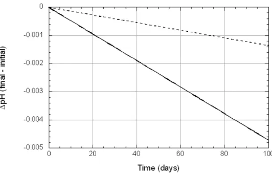
Calculated changes in the amount of smectite dissolved in dilute pore water (Experiment L1) and in 1 M NaOH (Experiment L2) over a period of 100 days (Model A) were minimal (Figure 8) and the compositions of both aque-ous solutions remained at conditions far from equilibrium (Figure 9), and the dissolution rate was therefore essentially controlled only by the rate constant and surface area, and, at pH > 10, by aOH-. Resultant changes in pH (Figure
10) were controlled by the dissolution rate and by hydrolysis of the released cations. Smectite dissolution consumes H+, whereas cation hydrolysis pro-duces H+ (e.g., Al3+ + 4H2O(l) = Al(OH)4
+ 4H+). The net result is a small reduction in pH in both the L1 (-0.005 pH units) and L2 (-0.001 pH units) solutions. These changes are much smaller than those observed experimen-tally (-0.2 and -2.5 pH units for L1 and L2, respectively), which confirms that smectite dissolution is a process of minor importance under laboratory timescales at neutral pH.
We next consider changes in solution chemistry that would occur if smectite were to continue to dissolve beyond 100 days up until the time equilibrium is achieved. The calculated amounts dissolved and corresponding changes in pH are shown in Figure 11 and Figure 12, respectively. As can be seen in the former, 7.2 years are required for equilibrium in L1, and 65 years in L2. Both durations are much longer than the experiments of [6]. Changes in pH are small (Figure 12), again suggesting that the effects of smectite dissolu-tion are relatively unimportant under these condidissolu-tions.
Figure 8. Calculated amounts of smectite dissolved in L1 pore water (solid line) and L2 pore water (dashed line) over a period of 100 days at 25C, 1 bar.
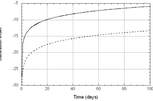
Figure 9. Calculated variations in the saturation index for smectite dissolu-tion in L1 pore water (solid line) and L2 pore water (dashed line) as a func-tion of time at 25C, 1 bar.
Figure 10. Calculated differences in pH during smectite dissolution in L1 pore water (solid line; initial pH = 9) and L2 pore water (dashed line; initial pH = 12.1) as a function of time at 25C, 1 bar.
Figure 11. Calculated amounts of smectite dissolved in L1 pore water (solid line) and L2 pore water (dashed line) over time periods required to achieve equilibrium (indicated by symbols) at 25C, 1 bar.
Figure 12. Calculated variations in pH as L1 pore water (solid line) and L2 pore water (dashed line) approach equilibrium with smectite at 25C, 1 bar (Model B).
Models A and B both assume that secondary minerals do not precipitate as smectite dissolves. Figure 13 indicates, however, that the aqueous concen-trations of Al, Fe and Si increase significantly as smectite approaches equi-librium with the L1 and L2 pore waters (Model B). Given these changes in solution chemistry, it seems reasonable to expect that insoluble secondary minerals (e.g. oxides, hydroxides, carbonates, aluminosilicates) will precipi-tate as smectite dissolves. This latter possibility is evaluated in Model C which represents a variant of Model B with the added provision that plausi-ble secondary minerals are allowed to precipitate under local equilibrium control if solution compositions evolve accordingly. The secondary miner-als considered in Model C are: kaolinite, calcite, goethite and sepiolite (rep-resenting a generic, insoluble Mg-bearing silicate) (L1 pore water); and anal-cime, albite, goethite, sepiolite, mesolite, siderite and pyrite (L2 pore water). Thermodynamic data for these minerals are included in Table 6. Given the general insolubility of aluminosilicate and other common types of secondary minerals, however, these illustrative effects are expected to be qualitatively similar to those that would be predicted using more realistic (kinetic) models of bentonite-pore water interactions. Goethite and pyrite are included in Model C because MX-80 smectite contains small amounts of both ferrous and ferric iron. Redox conditions are further constrained by assuming that the model system initially equilibrates with atmospheric O2(g) with pO2(g) =
Figure 13. Calculated changes in the concentrations of Al3+ (solid lines),
Fe (dashed lines) and SiO2(aq) (dotted lines) during dissolution of MX-80
smectite in dilute (L1) pore water (red lines) and 1 M NaOH (black lines). The terminus of each curve represents conditions at equilibrium (see Figure 11). Initial cation concentrations = 10-10 molal.
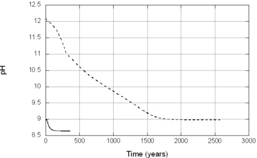
Figure 14 and Figure 15 depict changes in the amounts of smectite dissolved and secondary minerals precipitated as smectite equilibrates with the L1 and L2 pore waters, respectively. A striking feature of both Figures is that equilibration times are much longer than those predicted using Model B (360 years versus 7.2 years for L1 pore water; 2600 years versus 65 years for L2 pore water). Corresponding changes in pH (Figure 16) are also much more pronounced than those calculated using Model B. These results indicate that when the kinetic model of smectite dissolution is combined with plausible local-equilibrium constraints on the precipitation of secondary phases, pre-dicted changes in solution chemistry can be significant.
The Model C variant involving L2 pore water was further evaluated using an alternative value for the log K for hydrolysis of MX-80 smectite that was estimated using the approach of Vieillard ([22]). Results are shown in Figure 17 and Figure 18. The use of log K estimated using Vieillard’s tech-nique (log K = 4.4) in place of that estimated using the Polymer model (log K = 2.07) causes the time required for MX-80 smectite to equilibrate to in-crease from 2600 years to 5000 years. Changes in pH using these two dif-ferent log K values are identical under far-from-equilibrium conditions, but differ significantly as equilibrium is approached (Figure 18). The differ-ences reflect uncertainties in the thermodynamic properties of smectite. The results shown in Figure 18 suggest that this uncertainty can significantly affect models of the kinetic evolution of smectite-water reactions.
Figure 14. Variations in mineral abundances as dilute (L1) pore water equilibrates with MX-80 smectite. Equilibration time = 360 years.
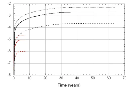
Figure 15. Variations in mineral abundances as alkaline (L2) pore water equilibrates with MX-80 smectite. Equilibration time = 2600 years.
Figure 16. Calculated changes in pH as L1 pore water (solid line) and L2 pore water (dashed line) approach equilibrium with smectite at 25C, 1 bar (Model C).
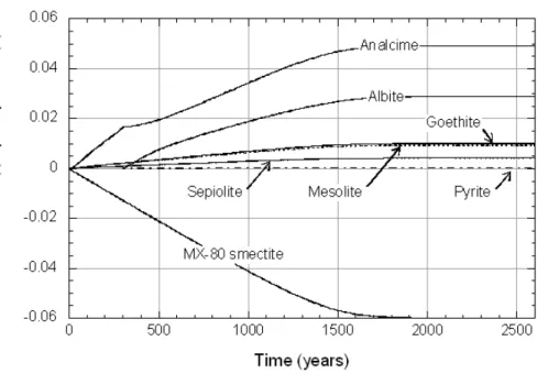
Figure 17. Variations in mineral abundances as alkaline (L2) pore water equilibrates with MX-80 smectite. The equilibrium constant for smectite dissolution estimated using the model of Vieillard ([22]) was used in this simulation in place of that estimated using the Polymer Model. Equilibra-tion time = 5000 years.
Figure 18. Comparison of pH evolution calculated in Model C (L2) using alternative log K values for MX-80 smectite dissolution. The solid line re-fers to calculations based on the Polymer Model (log K = 2.07), and the dashed line refers to calculations based on Vieillard’s technique (log K = 4.89).
5.3
Time- and space-dependent
cal-culations
The diffusion experiment ‘DIF6’ of Muurinen and Carlsson ([6], [19]) was modelled in time and space using the QPAC computer code ([40]), which has a fully coupled reactive-transport chemical module. A number of cases were set up and run, to investigate the effects of individual processes (such as secondary mineral precipitation, ion exchange etc.) on the system. A summary of the model cases is given in Table 10.
QPAC employs a finite volume approach. The model of the diffusion ex-periment was discretised using 19 compartments in the bentonite, ranging from 0.5 mm wide at the end exposed to the high-pH fluid, to 10 mm at the most distal end. The fluid reservoir was modelled as a single compartment. In order to represent the changes to the high-pH fluid in the reservoir, and the subsequent replenishment of the reservoir fluid, 7 separate reservoir compartments were used which were each connected to the bentonite in se-quence (by turning fluxes on and off). For the majority of cases considered, a very short diffusion length in the reservoir was considered (0.01 mm); however this did not always provide the best fit to the data, and was thus varied in some variant cases (to 1 mm or even 40 mm). This parameter can be thought of as quantifying how well-mixed the reservoir is; the shorter the length, the better mixed it is. Results from a selection of the model cases are discussed in the following sections.
Table 10. Summary of the model cases for the diffusion experiment DIF6. Case Secondary minerals Ion Ex-change Surface Com-plexation Porosity Model Analcime? Brucite Surface Area Reservoir mixing length
Smectite kinetics CO2(aq) ? Diffusion Coefficient
D Total N/A N/A 0.01 mm Sato 7.42e-11 m2 s-1
E1 Total 1e3 m2 g-1 0.01 mm Sato 7.42e-11 m2 s-1
E2 Total 1e3 m2 g-1 0.01 mm Sato 7.42e-11 m2 s-1
F Geochemical 1e3 m2 g-1 0.01 mm Sato 7.42e-11 m2 s-1
G1 Total 1e3 m2 g-1 0.01 mm Sato 7.42e-11 m2 s-1
G2 Total 1e3 m2 g-1 0.01 mm Sato 7.42e-11 m2 s-1
H1 Total 0.1 m2 g-1 0.01 mm Sato 7.42e-11 m2 s-1
H2 Total 0.1 m2 g-1 0.01 mm Sato 7.42e-11 m2 s-1
J1 Total 0.1 m2 g-1 1 mm Sato 7.42e-11 m2 s-1
J2 Total 0.1 m2 g-1 1 mm Sato 7.42e-11 m2 s-1
K1 Total 0.1 m2 g-1 40 mm Sato 7.42e-11 m2 s-1
K2 Total 0.1 m2 g-1 40 mm Sato 7.42e-11 m2 s-1
L1 Geochemical 0.1 m2 g-1 0.01 mm Sato 7.42e-11 m2 s-1
L2 Geochemical 0.1 m2 g-1 0.01 mm Sato 7.42e-11 m2 s-1
M1 Total 0.1 m2 g-1 0.01 mm Rozalen 7.42e-11 m2 s-1
M2 Total 0.1 m2 g-1 0.01 mm Rozalen 7.42e-11 m2 s-1
N1a Total 0.1 m2 g-1 0.01 mm Sato 7.42e-11 m2 s-1
N2b Total 0.1 m2 g-1 0.01 mm Sato 7.42e-11 m2 s-1
Q Total 0.1 m2 g-1 0.01 mm Sato 7.42e-12 m2 s-1
Rc Total 1e3 m2 g-1 1 mm Sato 7.42e-11 m2 s-1
a
Initial CO2(aq) concentration was 10-4.5 mol l-1. b
Initial CO2(aq) concentration was 10-3.5 mol l-1. c
The pH of the deionised water was artificially fixed at 8.4. Montmorillonite surface area increased by a factor of 10 (was 30 m2 g-1); that of analcime reduced to 18 m2 g-1 (from 1000 m2 g-1).
5.3.1
Case D – smectite hydrolysis only
In this case (the simplest of all the cases considered), the only process in-cluded was the hydrolysis of the primary minerals, using the kinetic data of Sato et al. ([30]) which formed the reference dataset for clay dissolution kinetics for the time- and space-dependent modelling. Figure 19 shows the evolution of pH at each of the measurement points in the sample and in the reservoir (symbols and dotted lines show the measured values, solid lines show the model output). As might be expected (and in support of calcula-tions described for Model A), there is no buffering of the pH and the whole system rapidly reaches a state of equilibrium such that the pH is the same throughout the sample and in the reservoir.
5.3.2
Cases E1 and E2 – inclusion of secondary
mineral growth
The additional process of kinetic secondary mineral precipitation was in-cluded in this case. If analcime is allowed to precipitate, the effect on the pH in the bentonite sample is marked, with a sharp decrease in pH (Figure 20). The pH at 5 mm depth remains between 9.5 and 10, but deeper into the sam-ple, pH decreases (fluctuating between about 7.5 and 9 as it responds to the replenishing of the reservoir). The modelled pH in the reservoir matches the experimental data well; in the bentonite sample the model only captures some of the most basic behaviour, though it is clear that the precipitation of secondary minerals is an important process in the buffering of the pH. A volume fraction plot for this case is shown in Figure 21 after 2 years of simulation. The high pH reservoir is located at the right-hand end of the plot. Large amounts of montmorillonite have dissolved in the first few mil-limetres, replaced by analcime and tobermorite.
Over lab timescales at 25 °C, it is thought unlikely that analcime will form. Therefore a second simulation was performed with this mineral removed; the pH evolution is shown in Figure 22. Although the pH is buffered a little compared to the case with no secondary mineral precipitation (c.f. Figure 19), the evolution at depth in the bentonite mirrors that at 5 mm. The most abundant mineral is tobermorite (with small amounts of brucite).
5.3.3
Case F – geochemical porosity model
A discussion of porosity models was given in Section 2. The previous runs used the total porosity; for this case the effects of using the ‘geochemical’ porosity are studied. Agreement with the experimental results was not good; the pH at all points in the bentonite decreased to a very low value (~7.5) after an initial spike in response to the introduction of high-pH fluid from the reservoir (Figure 23). This is due to the precipitation of the analcime and tobermorite which quickly blocks the limited porosity, inhibiting the trans-port of ions through the sample.
Figure 19. The evolution of pH for Case D (only mineral hydrolysis in-cluded).
Figure 20. The evolution of pH for Case E1 (primary mineral hydrolysis and secondary mineral precipitation).
Figure 21. Volume fraction plot for Case E1 at 2 years. The montmorillo-nite has dissolved near the incoming high-pH water (right-hand end); anal-cime and tobermorite have precipitated in its place.
Figure 22. The evolution of pH for Case E2 (primary mineral hydrolysis and secondary mineral precipitation, no analcime).
Figure 23. The evolution of pH for Case F (primary mineral hydrolysis, secondary mineral precipitation, and geochemical porosity).
5.3.4
Cases G1 and G2 – inclusion of ion
ex-change
These cases included ion exchange on the clay, as well as kinetic clay hy-drolysis and kinetic secondary precipitation (reverting to use of the total porosity). If analcime is included as a secondary mineral, there is a poor fit to the experimental data (Figure 24). In this case, brucite precipitates in larger quantities, along with analcime and tobermorite.
If analcime is omitted from the calculations, the results are closer to meas-ured values (Figure 25), but there is no initial spike in pH at 5 mm, and the pH values at 10 and 20 mm are greater than those measured. It is also noted that the pH of the reservoir is too low, especially near the start of the simula-tion.
Figure 24. The evolution of pH for Case G1 (primary mineral hydrolysis, secondary mineral precipitation and ion exchange).
Figure 25. The evolution of pH for Case G2 (primary mineral hydrolysis, secondary precipitation and ion exchange, no analcime).
Figure 26. The evolution of pH for Case 6a (primary dissolution, secondary mineral precipitation, ion exchange, slower brucite precipitation and a less well-mixed reservoir; no analcime).
5.3.5
Case J – increased reservoir mixing length
The ‘saw-tooth’ variation of pH in the reservoir reflects the periodic replen-ishment of the high pH fluid and then decrease of pH due to reaction-diffusion. By increasing the diffusion length in the reservoir to 1 mm (from 0.01 mm), it is possible to obtain a better fit to the pH evolution. In addition, it was found that the precipitation of brucite was very important in buffering the pH. Too much brucite and the pH was held at a low value throughout the bentonite (e.g. Figure 25); too little and there was no buffering capacity (e.g. Figure 19). Figure 26 shows the results from a case where the specific sur-face area of brucite has been reduced to 0.1 m2 g-1 (from 1000 m2 g-1), slow-ing its reaction rate.Although the simulation results remain an indifferent fit to the experimental data, some of the basic features are observed, e.g. an initial peak in pH and a buffering capability, with less response deeper into the bentonite (at least after ~500 days).
5.3.6
Case M – alternative kinetic model for
smec-tite
For this case, an alternative dataset for clay dissolution ([31]) was employed to describe the dissolution of montmorillonite (equation (6)). Ion exchange was also included, and the rate of brucite precipitation decreased as for case J. There was little difference between the pH evolution for this case and that for case J2, although the peaks in pH were larger and smoother in case M2 (Figure 27). However, a volume fraction plot (Figure 28) indicates that, after 2 years, there is negligible montmorillonite dissolution. Brucite is the dominant secondary mineral.
5.3.7
Case N – inclusion of CO
2(aq)A recurring feature of all the cases is that the initial pH in the bentonite is too great (about 9 compared to the value between 8 and 8.5 measured in the experiments). Although the experiment was conducted in a nitrogen glove box, and thus theoretically with the exclusion of CO2, the reported pH does
not seem to be consistent with a system with CO2 excluded. To test this,
CO2(aq) was introduced as an aqueous species with a concentration of 10-4.5
mol l-1 in the initial deionised water. In the high-pH water, it was taken to be at trace concentration. Model results showed that pH evolution is similar to case J2 (Figure 29), but as expected, the initial pH matches the experimental results more closely. Changes in calcite concentrations were minor in all runs and thus had negligible impact upon pH in accord with its dissolution reaction at elevated pH:
CaCO3 Ca2 CO32 (7)

![Figure 5. Summary of pH measurements in experiment L2 ([6], [19]). The composition of the final squeezed pore water (pH 12.1) is shown in Table 8](https://thumb-eu.123doks.com/thumbv2/5dokorg/3351655.19084/16.892.250.645.626.938/figure-summary-measurements-experiment-composition-final-squeezed-table.webp)
![Figure 6. Schematic diagram of the diffusion cell. From Muurinen and Carlsson ([6], [19])](https://thumb-eu.123doks.com/thumbv2/5dokorg/3351655.19084/17.892.286.620.110.505/figure-schematic-diagram-diffusion-cell-muurinen-carlsson.webp)
![Table 1. MX-80 composition. From [20], [6], and [19]. Measured wt % Simplified wt % Simplified vol % Montmorillonite 87 90 48.7104 Quartz, SiO 2 5 8.5921 4.8666](https://thumb-eu.123doks.com/thumbv2/5dokorg/3351655.19084/20.892.217.674.164.367/table-composition-measured-simplified-simplified-montmorillonite-quartz-sio.webp)