2002:18 A Review of Models for Dose Assessment Employed by SKB in the Renewed Safety Assessment for SFR 1

(1)

A Review of Models for

Dose Assessment Employed by SKB

in the Renewed Safety Assessment

for SFR 1

2002:18 GEORGE SHAW

(2)

SSI rapport : 2002:18 september 2002 ISSN 0282-4434 AUTHOR/ FÖRFATTARE: George Shaw

DIVISION/AVDELNING: Department of Waste Management and Environmental Protection/Avdelningen för avfall och miljö.

TITLE/ TITEL: A Review of Models for Dose Assessment Employed by SKB in the Renewed Safety Assessment for SFR 1/Granskning av modeller för dosberäkningar i SKB:s förnyade säkerhetsanalys för SFR 1.

SUMMARY: This document provides a critical review, on behalf of SSI, of the models employed by the Swedish Nuclear Fuel and Waste Management Co (SKB) for dose assessment in the renewed safety assessment for the final repository for radioactive operational waste (SFR 1) in Forsmark, Sweden.

The main objective of the review is to examine the models used by SKB for radiolo-gical dose assessment in a series of evolving biotopes in the vicinity of the Forsmark repository within a time frame beginning in 3000 AD and extending beyond 7500 AD. Five biosphere models (for coasts, lakes, agriculture, mires and wells) are des-cribed in Report TR-01-04. The principal consideration of the review is to determine whether these models are fit for the purpose of dose evaluation over the time frames involved and in the evolving sequence of biotopes specified. As well as providing ge-neral observations and comments on the modelling approach taken, six specific questions are addressed, as follows.

• Are the assumptions underlying the models justifiable ? • Are all reasonably foreseeable environmental

processes considered ?

• Has parameter uncertainty been sufficiently and reasonably addressed?

• Have sufficient models been used to address all reasonably foreseeable biotopes?

• Are the transitions between biotopes modelled adequately (specifically, are initial conditions for developing biotopes adequately specified by calculations for subsiding biotopes) ? • Have all critical radionuclides been identified ?

It is concluded that, in general, the assumptions underlying most of the models are justifiable. The exceptions are a) the rather simplistic approach taken in the Coastal Model and b) the lack of consideration of Ôwild’ foods and age-dependence when calculating exposures of humans to radionuclides via dietary pathways. Most fore-seeable processes appear to have been accounted for within the constraints of the models used, although it is recommended that attention be paid to future climate states when considering these processes. Parameter uncertainty has been addressed in detail for the existing models but numerous detailed recommendations are made for the improvement of several specific parameter selections. It is also recommended that two semi-natural ecosystem models (for forest and dry meadows) are included in the study – this would require further parameter identification and collection. Transitions between developing biotopes need more careful explanation and reaso-ning and EDFs (Ecosystem Dose Factors) for all ecosystem types should be presented to demonstrate more clearly that all critical radionuclides have been identified. SAMMANFATTNING: Denna rapport redovisar en kritisk granskning, som utförts på uppdrag av SSI, av de modeller SKB använt för dosberäkningar i den förnyade säker-hetsanalysen för slutförvaret för radioaktivt driftavfall i Forsmark, SFR 1. I rappor-ten granskas de fem biosfärsmodeller (kust, sjö, jordbruksmark, myrmark och brunn) som SKB använt för att beskriva successionen av olika biotoper i Forsmark-sområdet och beräkna radiologiska doser under en tidsperiod som sträcker sig bort-om 5500 år i framtiden. Granskningen har koncentrerats på att bestämma bort-om

(3)

modellerna är tillräckliga för sitt syfte att beräkna doser över dessa tidsperioder och för att beskriva den specificerade tidsutvecklingen av olika biotoper. Följande specifika frågor har särskilt beaktats:

• Är alla antaganden i de underliggande modellerna tillräckligt motiverade ?

• Har alla rimligt förutsägbara miljöprocesser tagits i beaktande ?

• Har osäkerheter i olika parametrar utvärderats så långt det är rimligt ?

• Är modellerna tillräckliga för att beskriva alla rimligt förutsägbara

biotoper ?

• Är övergångarna (i tiden) mellan olika biotoper adekvat beskrivna i modellerna ?

• Har alla kritiska radionuklider identifierats ?

Författarens slutsats är att de antaganden som ligger till grund för de flesta av mo-dellerna överlag kan rättfärdigas. Undantagen är a) de relativt stora förenklingar-na i kustmodellen och b) att man inte tagit hänsyn till förenklingar-naturlig föda (t.ex. vilt, bär, och svamp) och åldersberoende i beräkningarna av exponering till människor via födointag. Rimlig hänsyn tas till förutsägbara processer med hänsyn till de be-gränsningar som finns i modellerna. SKB rekommenderas dock att ta hänsyn till framtida klimatförhållanden när dessa processer beaktas. Parameterosäkerhet har hanterats utförligt i de använda modellerna. I rapporten ges dock ett antal mendationer på hur valet av specifika parametrar kan förbättras. Vidare rekom-menderas att två seminaturliga ekosystemmodeller (för skog och torr ängsmark) bör inkluderas i analyserna, vilket skulle kräva ytterligare identifiering av para-metrar och insamling av data. Hanteringen av övergångar mellan olika biotoper behöver förklaras och motiveras bättre och EDFs (ekosystemspecifika dosom-vandlingsfaktorer) bör presenteras för alla ekosystem för att tydliggöra att alla kritiska radionuklider har identifierats.

(4)

Förord

Svensk Kärnbränslehantering AB (SKB) redovisade sommaren 2001 en förnyad säkerhetsanalys av slutförvaret för radioaktivt driftavfall vid Forsmark, SFR 1, etapp 1. I SSI:s och Statens kärnkraftinspektions (SKI) drifttillstånd från 1988 och 1992 anges att SKB ska lämna en sådan uppdaterad analys till myndigheterna minst vart tionde år så länge förvaret är i drift. SSI och SKI har i sin gemensamma granskning av SKB:s säkerhetsredovisning för SFR 1, framförallt vad gäller förvarets skyddsförmåga efter förslutning, tagit hjälp av oberoende internationella experter som detaljgranskat viktiga delar av SKB:s säkerhetsredovisning.

Denna rapport redovisar en av flera konsultgranskningar av SKB:s säkerhetsredovisning för SFR 1, som utförts på uppdrag av SSI. Rapporten redovisar en fördjupad granskning av de mo-deller som SKB använt för att beskriva exponeringsvägar för radionuklider i olika ekosystem, och för beräkningar av vilka doser dessa radionuklider skulle kunna ge till människor. Detta är frågor som SSI har att ta ställning till bl.a. vid bedömningen av hur väl SKB:s säkerhetsredovis-ning för SFR 1 uppfyller SSI:s föreskrifter om slutligt omhändertagande av använt kärnbränsle och kärnavfall (SSI FS 1998:1).

Arbetet har utförts av George Shaw på Imperial College of Science Technology and Medicine i England, på uppdrag av Björn Dverstorp, avdelningen för avfall och miljö, SSI. Författaren svarar själv för innehållet i denna rapport. SSI:s samlade bedömning av SKB:s redovisning kommer att redovisas i en särskild granskningsrapport som tas fram gemensamt av myndighe-terna SSI och SKI.

(5)

1 Introduction

1.1 Background and objectives of review

This document provides a critical review, on behalf of SSI, of SKB Report TR-01-04 (Models for Dose Assessments – Models Adapted to the SFR Area, Sweden) produced for SKB and au-thored by S. Karlsson, U. Bergström and M. Meili (Karlsson et al., 2001).

The main objective of the review, based on a job description supplied by SSI in December 2001, is to examine the models used by SKB for radiological dose assessment in a series of evolving biotopes in the vicinity of the Forsmark repository within a time frame beginning in 3000 AD and extending beyond 7500 AD. Five relevant biosphere models (for coasts, lakes, agriculture, mires and wells) are described in Report TR-01-04. The principal consideration of this review is to determine whether these models are fit for the purpose of radiological dose evaluation over the time frames involved and in the evolving sequence of biotopes specified.

The six specific questions addressed are as follows.

• Are the assumptions underlying the models justifiable?

• Are all reasonably foreseeable environmental processes considered?

• Has parameter uncertainty been sufficiently and reasonably addressed?

• Have sufficient models been used to address all reasonably foreseeable biotopes?

• Are the transitions between biotopes modelled adequately (specifically, are initial conditions for developing biotopes adequately specified by calculations for subsiding biotopes)?

• Have all critical radionuclides been identified?

A specific review is also made of the comparison of sorption properties and contaminant path-ways described in Chapter 10 of TR-01-04. A review of the methods of dose calculation was considered from the outset to be of secondary importance as these are based on conventional techniques. However, as requested, the question of whether reasonable ranges of parameter values have been used in the calculations is addressed.

1.2 Structure of review

The review begins (Chapter 3) with some general observations and comments on the modelling approach taken in Report TR-01-04, together with some general recommendations for the im-provement of the clarity of presentation of the report. Chapter 4 summarises and describes the content of each of the chapters of TR-01-04 and provides general comments, where appropriate, on the specific assumptions, parameters and methods used in each chapter. Chapter 5 provides a general discussion of the report and considers, specifically, whether each of the six specific questions, above, have been addressed satisfactorily. Finally, Chapter 6 makes specific point-by-point recommendations for the general improvement of the report.

(7)

2 Comments on the modelling approach

used in the report

2.1 General

comments

The key problem in modelling radionuclide transfers, and the consequent radiological exposures of man, in ecosystems is the difficulty in finding an appropriate balance between model realism and model simplicity. The degree to which real-world processes are simplified within a model is usually dictated by the end use to which the model will be put. In other words, so long as a model can be demonstrated to be fit for purpose then it can be considered to be adequate. Usu-ally, it is necessary to carry out some form of model validation before it can be judged whether a model is, indeed, fit for purpose. In the context of the SFR assessment the validation of any model over the extremely long (1,000 to 10,000 year) assessment period is clearly impossible. Therefore, the next best strategy in demonstrating the general applicability of a model applied over this time scale is to ensure that model conceptualisation and parameter selection have both been rigorous. For model conceptualisation, this means that all reasonably foreseeable states of the environment and radionuclide transfer processes should have been identified and included in the model, or suite of models, to be used for the assessment. For parameter selection, both the absolute values and known or assumed uncertainties of parameters should be shown to be rea-sonable, based on existing information. These two considerations should both be key objectives for TR-01-04.

The general modelling approach taken throughout the assessment study is simple, though com-pletely consistent from one ecosystem to the next. Thus, all problems of radionuclide migration in marine, freshwater, and terrestrial ecosystems are conceptualised as transfers from one dis-crete compartment to the next with transfers being quantified as first order (i.e., time- and con-centration-independent) processes. More complex, physically based, modelling methods are available for each of the ecosystems addressed in the study. However, it would be difficult to defend the use of a mechanistic and highly site-specific modelling approach when the data re-quirements of such models are usually very demanding and the uncertainties surrounding the site itself (particularly when considering its future state) are considerable.

So, the basic modelling approach taken in TR-01-04 should be at least adequate for the purpose of the study if

• the way in which the models are conceived and applied is made clear (e.g., underlying as-sumptions, definition of inputs and sequence of calculations) and

• the selection and use of parameters is fully explained and justified.

In order to meet these two criteria it is essential that any caveats associated with either model configuration or parameters is made clear. The reader of the report should be provided with sufficient information to be able to decide, finally, whether the conclusions reached are reason-able and defensible. Above all, clarity of presentation of ideas and modelling operations is es-sential.

(8)

Before addressing each chapter of the report specifically, a few general comments and sugges-tions will be made which are intended to improve the clarity of chapters describing both the general characteristics of the model system and the individual models.

2.2 Suggestions for the improvement of clarity of modelling

descriptions

The primary problem to be addressed by the system of models proposed is that it should be able to simulate radionuclide transfers in a continuously changing sequence of ecosystems. This evolutionary sequence of biotopes is explained in Section 2.2 yet, considering the importance of this sequence, this section is rather short. In Section 2.4.1 of Lindgren et al. [2001, SKB Report R-01-18] a schematic description of the ‘reasonable biosphere development’ for SFR is shown as a diagram (Figure 2-2, page 17). It would be beneficial to include this diagram in report TR-01-04 to aid the description of scenarios as described in Section 2.2. Furthermore, a flow dia-gram should be added to show the sequence of model calculations in relation to the sequence of ecosystem evolution. A modified version of Figure 2-2 [R-01-18] could be drawn in which the stages in the evolutionary sequence in which the individual models are used is clearly indicated. In particular, the points at which one model ceases to be used and another begins should be shown. It could be that the boundaries between one modelling scenario and the next are not distinct but ‘fuzzy’, in which case there would be periods during which two models need to be used side-by-side. In any case, it is very important to show how the outputs of one model pro-vide an input to another – again, for clarity; this should be incorporated in a general flow dia-gram somewhere near the beginning of the report.

At the beginning of each chapter in which a model or sub-model is described (Chapters 3, 4, 5, 6, 7 and 8) it would be useful to have all the parameters listed together with their symbols and units. This would avoid confusion. For example, the terms ‘transfer coefficient’ and ‘rate con-stant’ are used interchangeably within the report. In the first Paragraph of Section 3.1 (page 16) the term ‘rate constant’ is used, but in the first equation following this Paragraph the symbol TC is used to denote ‘transfer coefficient’. This is confusing and possibly misleading. Also missing are any equation numbers that makes it difficult to refer to a specific equation. The adoption of a system of equation numbers based on the section in which the equation appears is recommended – e.g., the first equation in Chapter 3 would have the number 3.1.1.

In the individual diagrams of the models at the beginning of Chapters 3, 4, 5, 6 and 8 the arrows should be labelled to indicate which parameters are used to represent the fluxes between com-partments. The use of transfer coefficients is described in general terms in Chapter 2. However, at present it is difficult to determine which equations in each chapter refer to each arrow (flux) in the model flow diagrams. Each transfer coefficient is, at present, simply referred to as ‘TC’, which makes it impossible to distinguish between individual transfer coefficients. Subscripts should therefore be used to give a unique identity to each transfer coefficient. For example, for the transfer coefficient representing movement of water from the Model Area to ‘Grepen’ in Chapter 3, the identity could be denoted as TC15, representing flow of water from compartment

1 to 5. This might seem cumbersome but it would avoid potentially confusing statements such as ‘The water inflow to Grepen from the Baltic Sea is obtained from the same expression but the values for the Model Area are replaced by those for Grepen and the values for Grepen by those for the Baltic’ (page 16).

As far as general terminology is concerned, it would be less ambiguous to use the term ‘activity concentration’ rather than just concentration. Similarly, there are many points throughout the report at which either radionuclides or elements are referred to when, in most cases, these terms are being used interchangeably. Since the report deals with radionuclides this term should be used in preference to elements.

(9)

The report is generally very well referenced but the presentation of references in the text could be improved by removing the solidus before and after the reference – this is probably due to the use of an automatic referencing system such as Endnote, but it should be corrected.

(10)

3 Review of assumptions, parameters and

methods used in each chapter

3.1 Chapter 1 – Introduction

The primary objective of TR-01-04, is set out in Section 1. It is made clear that the purpose of the document is to provide a description of a model system developed to predict radiation doses to the most exposed individuals resulting from the long-term release of radionuclides from the SFR facility. The general geographical setting and history of the SFR facility at Forsmark is briefly described and the requirement of the operational license for renewed safety assessments every ten years, which is catered for by the SAFE project, is explained. This is useful since an obvious question, which might be posed by a reader unfamiliar with the SFR facility, is why safety assessments are being carried out after the beginning of the operation of the repository.

Background studies on the biosphere within the area of the SFR facility are described on page 7, though these appear to be solely concerned with coastal processes such as shore level rise and sedimentation. It is not immediately clear from this part of the report how ‘this material has been used for developing a model system for the area’ since this information only appears to relate to the Coastal Model described in Chapter 3.

It would also be helpful to state more clearly in the first section of the Introduction (page 7) that sub-objectives of Report TR-01-04 are

• to describe the types of biosphere addressed in the study (see comments in Section 3.1, above) and

• to investigate the effects of different sorption properties on radionuclide pathways in coastal, lake and agricultural ecosystems.

It would be useful to state at the outset why the second of these objectives was necessary – for example, is it because sorption (Kd) is such a universally sensitive parameter in all the models

developed? In its current form the introductory chapter gives no indication why only the effects of sorption on model outputs were explored and not the effects of any of the other parameters.

Section 1.1 provides a more detailed description of the characteristics of the coastal area near Forsmark. Given the present-day coastal conditions at the site it is reasonable that this descrip-tion should focus on these features. However, a brief descripdescrip-tion is also given on page 9 of the expected evolution of Öregrundsgrepen over the next 2,000 to 5,000 years. At the bottom of page 8 it is stated that ‘No agricultural areas occur in the near vicinity of the repository area and the amount of agricultural land is low in general (less than 10 % …)’. This is further emphasised at the top of page 9 where it is stated that ‘Large scale farming does not occur in this part of the region’. In view of these statements it is surprising that emphasis has been given to an agricul-tural scenario while forests have not been considered even though, in the present day, they cover 70 % of the land (see also detailed comments on Chapter 5, Section 4.5). Since, over the as-sessment period of 1,000 to 10,000 years, the study area will evolve from a coastal to a terres-trial environment that is likely to be dominated by semi-natural ecosystems, it would seem reasonable that more emphasis should be given to this type of biotope.

(11)

The major shortcoming of the description of the study area is the lack of any mention of climate change that is likely to occur in parallel with the evolution of the land surface over a period of 1,000 to 10,000 years from the present day. In developing a defensible system of models for future ecosystem states this information, even though it may be subject to large uncertainties, is extremely important.

3.2 Chapter 2 – General characteristics of the model system

Chapter 2 describes, in general terms, the characteristics of the models developed to carry out radiological assessments of radionuclides emerging from the SFR repository into the local bio-sphere. It is stated at the beginning that these models are based on those developed by Bergström et al. [1999] for safety assessment SR 97 and this gives the impression that the au-thors assume the reader of TR-01-04 will be familiar with this document. Since many readers will not be familiar with previous models developed for assessment of the SFR facility it would be useful if the authors started from this assumption and provided a clearer introduction to the models actually described in TR-01-04. This might be achieved by listing or tabulating the models actually used (Coastal, Lake, etc.) together with their common and individual features.

The description of the use of transfer coefficients and bioaccumulation factors for different model components might be made clearer for the non-expert reader if a generic model structure were proposed and described. This generic model structure should refer to the description of the long-term geochemical processes and shorter-term biological processes as currently described in the text, but the definitions and units of transfer coefficients and bioaccumulation factors should be given. For example, a generic model might consider sorption and desorption of radionuclides between solid and liquid (physical) phases followed by biological uptake from the soluble pha-se, see Figure 1.

The basic symbol and definition of the transfer coefficient should be given, for example:

year that during phase liquid in contained activity de radionucli Average year one during phase solid to phase liquid from moving activity de Radionucli TC=

and the units given:

1 -1 y y Bq TC = = − . Figure 1 Suggested diagrammatic description of a generic model structure to aid un-derstanding of the detailed model structures described in Chapters 3 to 8.

Bioconcentration factor

Solid

Phase Organism

Physical components Biological component Transfer coefficients

Liquid Phase

(12)

Thus, when more complex derivations of transfer coefficients are shown in specific modelling chapters (Chapters 3 to 8) the non-expert reader should understand that the dimension of the TC should be y-1 and that TCs are dynamic parameters. Similarly, the basic symbol and definition of the bioaccumulation factor should be given:

phase liquid in ion concentrat activity de radionucli Average organism of part or organism in ion concentrat activity de radionucli Average BCF=

and the units given:

less) (dimension kg Bq kg Bq BCF 1 --1 = .

Thus, the non-expert reader should understand that the BCF is a non-dynamic parameter, which assumes very rapid establishment of equilibrium of radionuclide activity concentrations between an organism and its environment.

Given the similarity in model structure between many of the models proposed in TR-01-04 the description of the generic ‘building blocks’ of the models should be straightforward and would significantly improve the clarity of Chapter 2.

Also described in Chapter 2 are the biosphere scenarios which, it is assumed, will apply to the study area over a period up to 12 000 AD (i.e., 10,000 years from the present day). The descrip-tion of these biosphere scenarios could be significantly improved to aid the reader’s understand-ing of the system of biotopes beunderstand-ing modelled. One way in which this could be achieved would be to show diagrammatically the predicted evolution of the site. In Section 3.1, above, it has already been suggested that Figure 2-2 within report R-01-18 could be adopted for use in TR-01-04. The reader’s understanding of the applicability of each of the models to each phase in the biosphere evolution would be further strengthened if each stage in this figure indicated clearly which model was applicable at each evolutionary phase. This would be made simpler if, as sug-gested above, a single table of each model and its major attributes were presented at the begin-ning of Chapter 2. One of the key problems in using a suite of discrete models to evaluate ra-dionuclide migration in each of the individual phases in the evolving biosphere is that transitions between phases are not easily represented. Some effort must, therefore, be made to show diagrammatically how the output from one model is used to represent the input to another model, as described verbally at the bottom of page 12 in TR-01-04.

Finally, justification of the well scenario, modelled in Chapter 7 of TR-01-04, needs to be im-proved. Is the granite/gneiss bedrock likely to be a useful aquifer and is the supply of water at the surface likely to be so limiting that a well is required to provide drinking and irrigation wa-ter? Such questions might be linked to considerations of future climate state but as previously stated; climate change has not been considered in the report.

3.3 Chapter 3 – Coastal model

The Coastal Model seeks to represent three interconnected, though distinct, water bodies of three markedly different scales, viz. the Model Area, Öregrundsgrepen and the Baltic Sea. De-spite the very marked differences in scale of each of these water bodies the conceptual approach taken for each one is the same. Each sub-area within the Coastal Model comprises water and sediment compartments, with sediments being divided into suspended and upper and lower bot-tom sediments.

(13)

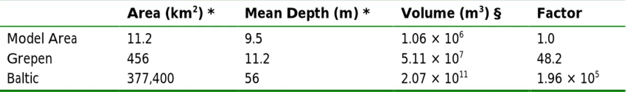
Table 1. Physical characteristics of the three major compartments considered by the Coastal Model. Area (km2_{) *} _{Mean Depth (m) *} _{Volume (m}3_{) §} _Factor

Model Area 11.2 9.5 1.06 × 106_1.0

Grepen 456 11.2 5.11 × 107_48.2

Baltic 377,400 56 2.07 × 1011 _{1.96 × 10}5

* Best estimates taken from Table 3-2. § calculated values.

The relative volumes of each of the compartments are shown in Table 1. The Model Area is ‘nested’ in the centre of Öregrundsgrepen. The water volume within Öregrundsgrepen is 48 times greater than the volume within the Model Area. However, due to the location of the Model Area within Öregrundsgrepen it is reasonable to assume a continuous exchange of water between the two areas.

The representation of the Baltic Sea in the same conceptual way as the two much smaller areas, however, is questionable. One of the fundamental assumptions of the compartmental modelling approach used throughout the report is that instantaneous mixing of radionuclides will occur in each compartment. The total volume of the Baltic Sea, calculated from the best estimates of sea surface area and mean depth presented in Table 3-2 (2.07×1011 m3), is almost 200,000 times greater than the Model Area itself and more than 4,000 times larger than Öregrundsgrepen.

A previously published model [Nielsen, 1995] treated the Baltic Sea as a series of horizontally and vertically stratified compartments. The region from Skagerrak in the west to the Belt Sea, south of Malmö, was treated as a series of five compartments (total volume 7.6×1012 m3) while the main part of the Baltic, east and north of the Belt Sea, was treated as a series of eight compartments (total volume 2.1× 1013 m3). Even with this degree of compartmentalisation, Nielsen [1995] admitted that the assumption of instantaneous uniform mixing could be a problem, especially close to the point of discharge where steep gradients in activity concentrations of radionuclides would be expected. This is the kind of problem, which would be expected when considering exchange of waters between the Baltic Sea and Öregrundsgrepen where the 4,000-fold difference in water volume would result in a very steep gradient in activity concentrations between the two compartments.

As might be expected, the mean water retention times of each of the three water bodies consid-ered are linearly related to the respective water volumes of the compartments (Figure 2). Thus, it would be expected that the radionuclide activity concentrations in the Model Area and Öre-grundsgrepen would reach steady state much more quickly than those in the Baltic Sea.

These problems are alluded to on page 21 for the scenario ‘Coast 2’. ‘… flux may be underesti-mated since the volume in the Baltic is too large and the water retention time may be too short’. It is also not clear which part of the Baltic Sea is being considered. Where does the boundary of the Baltic Sea and the ‘Oceans’ occur?

The problem of the comparative scaling of each of the three water bodies in the Coastal Model is perhaps best illustrated by Figure 10-1, Chapter 10, which shows that, at steady state, only a one to two order of magnitude difference in seawater activity concentrations is predicted be-tween the Model Area and the Baltic Sea – in reality, surely a bigger discrepancy bebe-tween

aver-age water activity concentrations in the Baltic Sea and Öregrundsgrepen would be expected?

Perhaps these modelling results are realistic? However, of all of the models proposed in TR-01-04 the coastal model seems to be the least justifiable in terms of the level of simplification it uses (see general comments at the beginning of Chapter 2, above). If the authors feel that this

(14)

All the equations in Chapter 3 have been examined and appear to be dimensionally consistent. However, as stated in Section 3.1, above, the equations need to be numbered consecutively and unique identities given to individual transfer coefficients.

All the parameter values used in the Coastal Model are shown clearly in Tables 3-2 and 3-3. These tables are both clearly presented and show parameter identifications, symbols, units and values (minima, best estimates and maxima). The system of footnotes used to identify the sources and to provide justification for the choices of individual parameter values is comprehen-sive although somewhat difficult to read. However, the use of detailed footnotes is good because it avoids the need for excessive cross-referencing of data sources in the main text of the chapter. One general criticism of these tables is that no key is given to identify the codes used to indicate the types of parameter distributions (Probability Density Functions) used.

The only parameter value, which appears open to question, is the maximum value for the depth of the upper sediment (Ds, 5 cm). From the text on page 18 this appears to represent the

maxi-mum depth of mixing by bioturbation as obtained from the reference by Eckhell et al. [2000]. Though not an expert in this specific field I would have considered that organisms such as ma-rine worms routinely burrowed below such depths and this might warrant a small discussion by the authors.

Related to the depth of mixing, as described on page 18 of TR-01-04, is the term ‘accumulation bottoms’ which is not sufficiently well defined for the non-expert reader to understand. This term should be defined more rigorously.

In summary, Chapter 3 presents a highly simplified model description of three water bodies of considerably different volumes and characteristics, but in each of which similar processes of sediment transport and radionuclide partitioning between solid and liquid phases can be ex-pected to occur. The simplicity of the conceptual model means that the selection of parameter values is made relatively straightforward and the selected parameters are evidently based on a sound body of site-specific studies which the authors have documented using detailed annotated footnotes. The major conceptual problem remains that the ‘Baltic Sea’ is represented as a single compartment when at least one previous study has represented the same sea area as a series of between 5–8 compartments. If the authors consider this level of simplification to be reasonable then a stronger justification is required, perhaps involving representative calculations using the Coastal Model in its current configuration.

1,0E-03 1,0E-02 1,0E-01 1,0E+00 1,0E+01 1,0E+02

1,0E+05 1,0E+06 1,0E+07 1,0E+08 1,0E+09 1,0E+10 1,0E+11 1,0E+12 Water Volume (m3) R e te nt ion Tim e ( y ) Figure 2

Water retention time versus water volume in each of the three areas represented in the Coastal Model.

(15)

3.4 Chapter 4 – Lake model

Conceptually, the Lake Model is identical to each of the three sub-components of the Coastal Model with water, suspended sediment, upper and lower bottom sediments being represented as discrete compartments. Inputs (X) and outputs of radionuclides are considered to occur directly into/from the water and suspended sediment compartments only.

In the first and second paragraphs of Chapter 4 it is stated that radionuclides may be present in the lake sediments due to deposition when the lake area was under marine conditions. However, a more explicit explanation of the transition from the Coastal Model to the Lake Model needs to be given. For example, how do the inputs ‘X’ into the water and suspended sediment compart-ments in Figure 4-1 relate to a) preceding contamination (especially of sediment) and b) current leakage from SFR? The relationship between outputs from the Coastal Model and inputs to the Lake Model could be explained using a general flow diagram, as suggested in Section 3.1, ex-plaining the sequence of evolution of the biosphere above SFR and the way in which each model is used to address each successive phase in this evolution.

All the equations in Chapter 4 appear to be dimensionally consistent. However, they need to be numbered consecutively and unique identities given to individual transfer coefficients. Essen-tially, the lake model is identical to each part of the Coastal Model representing a discrete water body. Consequently, the equations describing the transfer coefficients for the Lake Model are identical to those describing the transfer coefficients for the Coastal Model and the descriptions of each of the equations and parameters are very similar. Much of the model description in Chapter 4 could be considered redundant, therefore, unless the transfer coefficients are given unique identities as suggested in Section 3.1, above.

The main difference between Chapters 3 and 4 is the choice of parameter values. As in Chapter 3, many of the parameter values selected have been obtained from site-specific studies which are directly relevant to the SFR study area. An exception to this, however, is the choice of solid-liquid Kd values that are tabulated in Appendix 9. Of these values the ranges adopted are all

drawn from respected sources and it would be difficult to criticise these values. For Cs and Pu, however, I would suggest that the current maximum values (102 and 103, respectively) each be increased by one order of magnitude to 103 and 104. For Tc, the probability that chemical reduc-tion of this element will occur in anoxic bottom sediments dictates that a maximum Kd of the

order of 102 should be considered under these circumstances.

Table 4-1 is clearly presented and, as in Chapter 3, the system of footnotes is comprehensive. However, Table 4-1 needs a key to identify the codes used to indicate the types of parameter distributions (Probability Density Functions) used.

The bioaccumulation factors (BAFs) shown in Table A-13 are drawn from a variety of sources, most of which appear to be internationally recognised [e.g., IAEA, 1994]. It is curious that val-ues for BAFs for palladium for fish are based on an assumption of the similarity of uptake of nickel and palladium during plant root uptake. Some justification is given for this assumption in footnote 5 of Table A-13, but if palladium proves to be a critical radionuclide then these BAF values need more careful scrutiny. It is also noteworthy that the BAF values for crustaceans (Table A-15) are drawn from one source only [Thompson et al., 1972]. If consumption of crus-taceans proves to be a significant exposure pathway then it would be wise examine the literature for further sources of information on appropriate BAFs.

Finally, crop translocation factors are used when considering irrigation of crops with contami-nated lake water. These translocation factors are shown in Table A-6 and, for most elements

(16)

secondary source – a recent survey by ANDRA (pers. comm.) found no measured values for the Tc translocation factor in the literature.

3.5 Chapter 5 – Agricultural land model

The first impression of the structure of the soil model is its similarity to the aquatic models. Conceptually, this is reasonable, however, since it can be argued that both soils and aquatic (water/sediment) systems are similar to solid-liquid systems but with different ratios of solid to liquid components. Perhaps the most curious aspect of the Agricultural Land Model, however, is that it has been included in the study at all! In the first paragraph of Chapter 5 it is stated that ‘there will most probably not be any large areas suitable for cultivation of crops in the future’. This could be interpreted to mean that agriculture will be almost insignificant in the SFR area in future. In an area in which agriculture is almost insignificant it would be expected that any existing agriculture would be primitive, so the assumptions made about practices such as tile drainage on page 31 need to be justified.

As in the case of the Lake Model, a weak point in the general description of the Agricultural Land Model is the lack of any detailed explanation of how the predictions of the Coastal and Lake Models are used to provide inputs to the soil. A general statement that ‘Radionuclides accumulated in the sediments during the coastal and lake stage(s) are present within the soil as a secondary source’ is made (page 31) but more detail is required for clarity. Paragraph 3, page 31, states that ‘The fraction accumulated during the lake stage is present in the top soil layer whereas those from the coastal stages are added to the deep soil and the solid fraction of the saturated zone’. This is useful but a more explicit (e.g., diagrammatic) description of how one model’s output values provide input values into a subsequent model would greatly facilitate the reader’s understanding of the way in which the system of models operates.

Another important issue concerning the Agricultural Land Model concerns agricultural prac-tices. A lake sediment does not immediately become a cultivable soil for agriculture when the lake is drained and a major question is what effect the practice of preparing the soil for cultiva-tion (e.g., ditch or tile drainage as mencultiva-tioned on page 31) is likely to have on the radionuclide pool within the soil? Another question concerns direct inputs from the SFR facility into the groundwater and, ultimately, the topsoil. Paragraph 2 on page 31 suggests that the major sources of soil contamination with radionuclides will be the remains of contaminated lake sediments, as mentioned above, but it is also stated that ‘inflow of radionuclides with groundwater may also be simulated’. Such questions need to be addressed to improve the credibility of the model simulations.

The equations have been checked for dimensional consistency and appear to be correct. It is interesting that, unlike the Coastal and Lake models, the number of site-specific parameter val-ues available for the Agricultural Land Model is rather limited. Despite the fact that the parame-ter values selected are from a wide variety of sources, the choices of values seem generally judi-cious and are well justified. One potentially questionable value is the area assumed to be subject to agricultural use. A best estimate of 530,000 m2 is based on the assumption that half the area of Lake 4, as described in Chapter 4, is used for agriculture. Given the rather low percentage of land currently used for agriculture in the Forsmark area (less than 10 % according to Brunberg and Blomqvist [1998]) it would be useful to calculate the percentage of the assessment area which 530,000 m2 represents. If this is substantially more than 10 % of the total area it could be considered that the calculations of exposure via agriculture are unnecessarily pessimistic.

The effects on root uptake of crop species, soil type, climate and cultivation practices described on page 38 should be taken into account by the ranges of root uptake factors (RUFs) presented in tables A2 to A5 for pasture, cereals, root crops and vegetables, respectively. The RUFs pre-sented in these tables are well referenced and appear to be, in general, from internationally

(17)

rec-ognised sources. It would have been useful, however, to have stated which soil type has been assumed for the agricultural scenario. This can have a significant effect on the choice of RUF, but it is impossible to determine from the information provided whether this factor has been taken into account explicitly.

3.6 Chapter 6 – Mire model

As stated by the authors at the beginning of Chapter 6, the Mire Model is very simple – perhaps surprisingly so. Within the proposed model structure no account is taken of the process of peat formation and growth, which will be highly significant during the 1,000 to 10,000 years consid-ered in the assessment study. This leads to a problem because it is stated that ‘it can be assumed that the radionuclides are present within the peat at the start of modelling as a consequence of earlier accumulation in sediments’. The authors appear to be confusing peat with sediment: in fact, they are two entirely different materials with different modes of formation. Since peat is formed from organic matter, largely derived from atmospheric carbon, any radionuclides origi-nally incorporated in the ‘peat’ will be successively diluted as peat accumulation proceeds. This dilution may be balanced by further radionuclide accumulation in inflowing water (which is accounted for in the existing model) but the model would be more credible if it were to account for peat growth. A simple peat accumulation rate (kg DW m-2 y-1) could be adopted for this pur-pose using values that are applicable to present day and future climate conditions in Sweden.

Again, the existing equations appear dimensionally consistent and assumed correlations be-tween parameters appear reasonable. The authors admit that the ranges of parameter values adopted are generally wide and that they ‘should be seen as rough estimates’. Given this general limitation to the parameter estimates the ranges of values selected seem reasonable. Kd values

appropriate to organic soils are given in Table A-8. It is strongly recommend that values ob-tained from source 4 [IAEA, 1994] are re-checked by the authors. Several of the maximum val-ues quoted in Table A-8 are substantially below the valval-ues recommended for organic soils by the IAEA [1994]. For example, the maximum value recommended in Table A-8 for Pu is 20, while the corresponding maximum value suggested by the IAEA is 3.3 × 105. The authors of TR-01-04 may have good reasons for selecting lower values but these need to be justified.

In Section 6.4 of TR-01-04 it is stated that ‘the same root uptake factors (RUFs) as in the agri-cultural land model’ are used within the Mire Model to calculate root uptake of radionuclides by crops consumed by both humans and cattle. In Section 4.5, above, it was pointed out that soil type is important when selecting ranges of RUFs and, therefore, that a stronger justification should be given for the selection of RUFs in Tables A-2 to A-5 based on soil type. In my opin-ion, it is incorrect to assume that the soil types in the agricultural land scenario and the mire scenario are the same. Mire soils (peats) are likely to have more substantially organic matter contents than typical agricultural soils, even if the agricultural soil is derived from lake bottom sediments as assumed in Chapter 5 of TR-01-04. Therefore, RUF values for use in the Mire Model should be selected for predominantly organic soils – such value are available from sources such as IAEA [1994].

3.7 Chapter 7 – Well model

The major question which can be asked of Chapter 7 is the realism of a scenario in which a well is sunk into granite/gneiss bedrock (a very poor aquifer, which, presumably, is one of the main reasons why the SFR facility has been sited here) to provide irrigation water in a geographical area which is never likely to experience any significant limitation of the surface water supply.

(18)

of parameter values is that no initial justification is given as to the assumed lifestyle of people extracting and using the well water. The assumptions about personal water use and the use of water for animals and a garden plot appear to be based on present day practices. These assump-tion are acceptable if they are stated clearly at the outset but, at present, Chapter 7 makes no attempt to describe the type of domestic and/or farming system expected to be making use of well water. Future climate states will have a marked effect on this issue so the discussion of the well model parameters should be linked to a discussion of future climate (see comments in Sec-tion 4.1, above).

Well abstraction and irrigation scenarios generally lead to pessimistic predictions of exposures to sub-surface sources of radionuclide and, for this reason, they are often included in assessment calculations. If the primary reason for including the well water abstraction scenario in the SFR assessment is for the sake of pessimism then this should be stated.

3.8 Chapter 8 – Sub-model irrigation

The closing remarks in Section 4.7, above, apply equally to Chapter 8 in TR-01-04, which is devoted to the Irrigation Sub-Model. The main criticism of this chapter is that no justification is given for the inclusion of this sub-model. The use of the model in the assessment study needs to be justified in relation to likely domestic practices foreseen for the area, most probably based on current practices (it is stated on page 45 of TR-01-04 that irrigation of fields is not considered). It would be helpful at the outset of Chapter 8 to indicate whether irrigation of either agriculture or garden plots is a significant practice in the Forsmark area in the present day. If this is not the case then it seems unlikely that it will become a significant practice in future unless a future drier climate state is foreseen. This further emphasises the point, originally made in Section 4.1 above, that some prognosis or assumption of future climate states in the area is required in order to base the biosphere scenarios developed on a firmer footing. It is stated on page 45 that ‘The need for irrigation is, of course, governed by the water need of the vegetation and the annual precipitation’. This implies a close link with climate, but this needs to be stated formally.

The equations presented to describe irrigation and turnover in the soil are appropriate and di-mensionally consistent. It is stated on page 48 that ‘few site-specific data is used’ and that pa-rameter values from Bergström et al. [1999] have been adopted. Presumably these papa-rameter values are generic. In general the parameter values presented in Table 8-1 are reasonable and well documented with references and footnotes. However, I would question the initial retention of irrigation water on plant surfaces as described in Section 8.2. It is stated on page 46 that a 3 mm layer of water is assumed to be retained on a plant surface after an irrigation event. This is the product of a 0.5 mm storage capacity and a leaf area index (LAI) of 6. The LAI of 6 might be applicable to a small tree but it is possibly a factor of 5 times too high for a crop canopy – thus, the model probably overestimates significantly the importance of the direct contamination of crop foliage when calculating radiation exposure. Similarly, the area assumed to be irrigated (530,000 m2, in other words half the area of ‘Lake 4’) is extremely large for a garden plot. This is the same area assumed for the Agricultural Land Model as described in Section 4.5, above. Since the assumption made at the beginning of Chapter 8 is that irrigation to garden plots only is considered then it should be expected that the area affected should be significantly smaller than the area considered in an agricultural scenario.

In summary, the consistency of the application of each of the models could be improved by clearer development of scenarios – this is demonstrated particularly by the Irrigation Sub-Model, which needs to be based on firmer and more explicit assumptions.

(19)

3.9 Chapter 9 – Methods for calculation of doses to humans

It is not the purpose of this review to comment in detail on the methods used in TR-01-04 to calculate doses to humans since these methods are commonly used and accepted in assessments of this kind. The main requirement is to comment on the parameter values adopted for use in these calculations.

First, however, it is clear that Chapter 9 does not develop calculations solely for exposure to inhalation, ingestion and external sources. Sections 9.1.1, 9.1.2 and 9.1.3 (pages 54 to 58) actu-ally describe calculations of radionuclide contamination of animal, crop products and aquatic food products, respectively, rather than addressing directly the dose calculations via these prod-ucts. It would be better to include the descriptions of these calculations as part of the relevant sections in the preceding modelling chapters since the endpoints of ecosystem models should be radionuclide activity concentrations in compartments or food substances which can result in exposure of humans. Chapter 9 should deal with the exposure calculations (i.e., the application of appropriate dose coefficients) only.

The first major assumption in Chapter 9 is that all food products consumed by inhabitants of the study area are obtained from the local area. This is conservative, based on current Swedish hab-its, as explained by the authors, but it is reasonable since no assumptions are made about life-style habits of the local population over the next 1,000 to 10,000 years (see Section 4.7, above). Figure 9-1 shows the accepted pathways of human exposure to radionuclides in the environment and food products, but it could be improved by the addition of arrows that indicate that the vari-ous food products shown represent exposure via the dietary pathway. Also, a rather obvivari-ous feature of Figure 9-1 is that it shows ‘wild’ food products in the form of mushrooms and game, although these items are very clearly omitted from the assessment calculations described in Chapter 9. These items should either be omitted from Figure 9-1 or, preferably, they should be included as food products in the assessment of dietary exposure. This would, of course, necessi-tate the addition of models of semi-natural ecosystems to the suite of models already developed (see Section 5.4, below).

In terms of the pathways considered in the study, Table 9-1 is very useful as it clearly shows the individual exposure pathways relevant to each modelling scenario. This is a good example of how simple explanatory tables and figures can be used to improve the clarity of understanding, especially for non-expert readers, as discussed in Section 3.2, above.

Section 9.1.3 (page 58) provides a much better explanation of the applicability of bioaccumula-tion factors than currently given earlier in the report in Chapter 2 (page 11). It has already been suggested, in Section 4.2 above, that the description and definition of the bioaccumulation factor should be improved in Chapter 2.

As in previous chapters, the tabulated parameter values in Chapter 9 (Tables 9-2 to 9-5) are clearly set out and justified by extensive cross-referencing to published literature sources. The main question that arises concerning parameter value selections concerns Table 9-3 which shows parameters connected with human exposure. The first concern is that age-dependence of a) exposure and b) dose conversion coefficients is not mentioned. The authors need to specify which age group (or groups) they have considered in their study and adjust their choices of pa-rameter values accordingly. For instance, food, water and soil consumption rates by humans are all highly age-dependent. The authors state at footnote 2 of Table 9-3 that ‘No extreme diets are considered in this study so a relatively narrow range (i.e., a standard deviation of 10 % on all dietary consumption parameters) is used’. The assumption of ‘no extreme diets’ does not take into account the well known age-related range of dietary intakes, nor does it account for the

(20)

dict dose rates to the most exposed individuals’ it is therefore necessary to include such food products in the assessment calculations.

Another problem with the assumption of a 10 % standard deviation in Table 9-3 is that many ingestion rates, e.g., the ingestion of soil by children, are positively skewed and cannot be de-scribed by the adoption of a normal distribution – in fact a log-normal distribution is probably the best model. In a study by Stanek et al. [2001] it was shown that soil ingestion by children could be described by a log-normal distribution with a median value of 13 mg d-1. The current best estimate for soil ingestion in Table 9-3 (100 g y-1) is 21 times higher than the median value determined by Stanek et al. [2001] – this is pessimistic, but possibly unreasonably high.

Finally, on the question of age-dependence of dose parameters for dose calculations, it is not stated in Table A-1 to which age group(s) the dose conversion coefficients shown refer. If an assumption has been made by the authors to select a representative age group for the study, or if average dose conversion coefficient values have been calculated, then this should be stated clearly at the beginning of Chapter 9.

3.10 Chapter 10 – Effects of different sorption properties and

contamination pathways

Chapter 10 is the only chapter in Report TR-01-04 in which model simulations are shown. The first observation that can be made of these simulations is that they are all deterministic whereas it was previously described (page 12) that probabilistic model calculations (1,000 realizations) were to be made using the ranges and distributions of parameter values presented in the tables in each modelling chapter. For the purposes of Chapter 10, which is an analysis of the sensitivity of the models to solid-liquid Kd values, it may be the case that deterministic calculations are

more informative. However, it would also be useful to show at least some examples of the out-puts from probabilistic calculations in which Kd values are sampled from a continuous

distribu-tion of values.

The second observation concerns the use of a constant release of 10 kBq y-1 over a period of 1,000 years (page 63) when using the Coastal Model. Although it is not essential to the analysis of the effect of Kd (because the models all assume linear, concentration independent behaviour)

it would be useful to know on what basis this release rate was selected. Is it, for instance, based on a calculated release that may have been published in a previous report?

The general result achieved using the Coastal Model, as described in paragraph 2 on page 63, is reasonable. Can the results of these model simulations be supported by referring to real data, such as the experience in the Irish Sea in which Pu isotopes released from Sellafield have re-mained largely contained in the bottom sediments but from which Tc-99 has been largely lost to the North Atlantic and arctic seas? While this would not provide a direct validation of the Coastal Model it would indicate whether, broadly, the simulations were reasonable. Such a qualitative demonstration of the applicability of the Coastal Model is particularly desirable in the light of the criticism concerning the model’s simplicity as described in Section 4.3, above. It is stated in paragraph 2 on page 63 of TR-01-04 that ‘Even after reaching a steady state, the concentration of these elements will decrease with the distance from the outflow point due to dilution with clean waters and suspended matter entering the Baltic’. This is an important point because the gradient of concentration away from the release point will drive migration of ra-dionuclides away from the study area. However, in its current configuration it could be argued that the Coastal Model does not simulate this gradient sufficiently because it treats the entire Baltic Sea as one mixed compartment.

The important transition between the marine phase and the terrestrial phase is dealt with in the final paragraph on page 63. Here it is stated that ‘Elements with a strong tendency to sorb to

(21)

solid matter in the marine environment can be expected to show the same behaviour in soil’. This is questionable since the ionic strength of sea water is so much greater than that of an aver-age soil solution that de-sorption of elements such as Cs would be expected to be much greater in sea water [Assinder et al., 1985].

The results of the sensitivity analysis are clearly shown in Figures 10-2 to 10-4 that indicate that the Kd is, indeed, a very important parameter in the Coastal Model. It would have been useful,

however, to state at the beginning of Chapter 10 why this sensitivity analysis was so important that it requires a complete chapter. This shortcoming was identified in Section 4.1, above, and the reason for devoting Chapter 10 to this sensitivity analysis should, perhaps, be explained at the beginning of the report (i.e., Chapter 1).

The sensitivity analysis of the Lake Model is somewhat simpler since the model only comprise one third of the compartments, which make up the Coastal Model. The same release scenario of 10 kBq y-1 over a period of 1,000 years has been adopted as in the Coastal Model, but the re-lease is assumed to take place directly into the lake water. Again, the rationale for this scenario should be explained, even if it is not based on a calculated release from the SFR repository.

The results of the sensitivity analysis are clearly shown in Figures 10-6 to 10-8 that indicate that the Kd is also a very important parameter in the Lake Model. It is stated in paragraph 1 on page

69 of TR-01-04 that ‘The fraction of radionuclides sorbing to suspended matter increased with increasing Kd and as a consequence the fraction of the radionuclides leaving the lake sorbed to

particles compared to those leaving with the water also increased. With a Kd-value of 1,000

m3/kg the outflowing fraction associated with suspended matter is about twice the size of the dissolved fraction leaving the system’. However, as Kd increases, the total activity of

radionu-clides (soluble plus sorbed) leaving the lake decreases from 99 % to 23 % – this should also be pointed out in the text.

In the final paragraph on page 69 the discussion concerning the effect of irrigation in transfer-ring radionuclides from the lake to the soil is interesting but a simulation ‘was not included since the fraction removed is very small and insignificant’. However, it is later stated that ‘the levels of radionuclides in soils should increase due to a continuous build-up’. If continuous irri-gation over a period of 1,000 years is, indeed, a likely scenario (see Section 4.8, above) then a continuous build-up of radioactivity in the soil could be significant over such a long period. For this reason it would be useful to include a simulation of this build-up as part of Section 10.2 in the report.

Section 10.2.1 is an important part of the report since it deals with the transition of one bio-sphere model to another, which is probably the most difficult, and least well-explained aspect of the modelling study. From page 72 to page 75 a detailed argument is developed to test the hy-pothesis that radionuclides in deep sediments, originating under marine conditions, can diffuse upwards into lake water and increase the activity concentration in the lake water significantly. At the top of page 75 it is concluded that, even though this process occurs, it is not significant in terms of elevating the activity concentration in lake water so ‘Instead, radionuclides accumu-lated in the sediments during the lake stage were added to the pool which was used as a source in the agricultural land model’. It is useful that the authors have considered in such detail the transition from marine to lake sediment, but it would also be useful if they were to consider the transition from lake sediment to soil in similar detail. Such a consideration might, in particular, take into account any agricultural practices that are employed to convert lake sediment into cul-tivable soil, as pointed out in Section 4.5, above.

(22)

Section 10.2 it is stated that ‘Lower Kd-values were used compared to the tests with the coastal

and lake models since soil Kd is typically lower than sediment Kd’. This is a highly contentious

statement since the Kd in soil is highly dependent on soil type. In lines 13–15 of page 77 it is

stated that ‘…the masses of the different compartments in the model are different from what is gained when using the figures in Table 5-1…’. The reason for this should be explained, or if it is because ‘The calculations presented in this chapter were performed before the values of all pa-rameters were finally decided’, as the text goes on to say, then this should be more clearly stated.

In Figure 10-12 the very high values for radionuclide transfers between the solid and liquid phases in the groundwater are evident. The legend states that ‘The large figures for the transfers between the solid matter and groundwater in the saturated zone is a consequence of the large number of time steps used when solving the differential equations…’. Surely, it is not the large number of time steps per se but the fact that the sorption and desorption rates are relatively fast which gives rise to the very large interchange of radionuclides between soluble and sorbed phases over the end of a 10,000 year period? For instance, interchange of radionuclides between the saturated zone and the deep soil is calculated using the same number of time steps but the overall transfers are much lower.

On page 79, lines 4 to 5 state ‘This is an example of a non-linear response to a gradual parame-ter change, which may be difficult to predict without the use of complex and dynamic models’. This is an interesting point concerning the use of relatively simple linear models for long-term predictions. In view of this effect it would be useful if the authors were to discuss the possible shortcomings of the linear compartmental modelling approach when modelling systems that are inevitably subject to non-linear processes such as diffusion (see general comments concerning the general modelling approach used, Section 3.1, above).

Finally, it is interesting that the Agricultural Soil Model had not reached equilibrium even after a simulation period of 10,000 years. A comment from the authors on whether this would be expected in reality, even if the agricultural soil ecosystem were to remain constant over the simulation period, would be appropriate. Indeed, based on the site-specific studies [e.g., Kaut-sky, 2001] cited by the authors on the long-term development of biotopes in the vicinity of the SFR facility it would be useful if the authors were to comment on the applicability of the time-scales (1,000 and 10,000 years, respectively) examined in the sensitivity analyses described in Chapter 10.

3.11 Chapter 11 – Summary and discussion

The test simulations reported in Chapter 10 are summarised in the first paragraph of Chapter 11. One of the key conclusions is that ‘most of the radionuclides leave the Model Area and Öre-grundsgrepen quickly as a result of the fast water turnover’. This is not unexpected since the neighbouring water body, the major part of he Baltic Sea, is a large mass of water that provides a considerable sink for radionuclides emanating from the study area. Nevertheless, with the Coastal Model in its current configuration the results from the simulations are open to question because of the rather simplistic representation of the Baltic Sea as a single large compartment.

In Section 11.1 the authors describe the parameters used in the biosphere models based on the general categories to which they belong (geometrical, physical/chemical, etc.). It would have been useful to have described and categorised the nature of the parameters much earlier in the report, preferably when the general characteristics of the model system were described in Chap-ter 2. It is suggested in Section 4.2, above, that a generic model structure (e.g., Figure 1, above) is presented to facilitate the general description of the modelling approach used throughout the study. It would be most appropriate to discuss the general nature of parameters, and how they relate to such a generic model structure, at this point in the report.

(23)

The discussion comparing the relative uncertainties of each parameter type is very useful. It would also be useful to rank the parameter types based on their uncertainties, as follows.

radiological<geometrical<physical/chemical<biological<living habits

This is informative because it immediately alerts the reader to the fact that it is most probably the least technical data (i.e., living habits) that are subject to the greatest uncertainty while many of the more technical parameters can be quantified with greater certainty. It could be argued that, if present day living habits are assumed, these are not subject to such great uncertainty. However, it is noticeable that the authors have not made any comment about the likely foresee-able living habits of people or agricultural animals over the 1,000 to 10,000 year assessment period. It would be useful in Chapter 11 for the authors to address this question in more detail.

Section 11.2 compares, briefly, the results of the study reported in TR-01-04 with two previous studies, both conducted by at least one of the authors of the current report. At this point the con-cept of the ecosystem-specific dose factor is introduced. This is referred to as the Ecosystem Dose Factor (EDF) in both SR 97 and TR-01-04 and the EDFs calculated using the Coastal Model in TR-01-04 are presented in Appendix B. The Coastal Model EDFs are presented to facilitate comparison of the present study with the former studies, but it would also have been useful to present EDFs for the other models in the present study. Since EDFs are, by definition, ecosystem-specific, significant differences would be expected between EDFs calculated for different ecosystems!

It seems curious that EDFs for Co-60 and Cs-137 are discussed in the context of an assessment study lasting between 1,000 and 10,000 years since the short radioactive half lives of these ra-dionuclides would ensure that effectively complete radioactive decay would have occurred within 50 and 300 years, respectively. EDFs for the Lake Model are referred to on page 85 al-though no EDF values for this model are actually tabulated anywhere in the report. It would be useful to tabulate all EDFs calculated using each of the models.

The comparison of EDFs calculated using the different models used in TR-01-04 and SR 97 is interesting from the point of view not only of parameter uncertainty but of model uncertainty. In paragraph 2 of page 85 it is stated that ‘The main difference between the two (lake) models … is how sedimentation and resuspension processes are described…’. This statement makes it clear that model uncertainty contributes significantly to uncertainty in the EDF values obtained. This is fully to be expected but it is something which must be identified and discussed clearly when summarizing the results of this study.

Finally, on page 85 it would be most useful to have a clear concluding summary of the study, perhaps using bullet points to identify the key achievements of this study. The final paragraph of Chapter 11, which discusses the ecosystem based modelling approach developed by Kumblad [2001], is useful and interesting but it does not adequately conclude the main content of TR-01-04 which is the development and application of scenarios and models for assessment of the full range of possible biotopes which are expected to evolve around the SFR study area. It is argu-able that the ecosystem based modelling approach could not be used for this full range of sce-narios and biotopes so its use in future assessments may have to be carefully targeted at specific scenarios.