Article type: Original Article Published under the CC-BY4.0 license
Open and reproducible analysis: Yes Open reviews and editorial process: Yes
Preregistration: N/A
Analysis reproduced by: André Kalmendal All supplementary files can be accessed at OSF: http://doi.org//10.17605/OSF.IO/B5CXQ
Issues, Problems and Potential Solutions
when Simulating Continuous, Non-normal
Data in the Social Sciences
Oscar L. Olvera Astivia
University of Washington
Abstract
Computer simulations have become one of the most prominent tools for methodologists in the social sciences to evaluate the properties of their statistical techniques and to offer best practice recommendations. Amongst the many uses of computer simulations, evaluating the robustness of methods to their assumptions, particularly uni-variate or multiuni-variate normality, is crucial to ensure the appropriateness of data analysis. In order to accomplish this, quantitative researchers need to be able to generate data where they have a degree of control over its non-normal properties. Even though great advances have been achieved in statistical theory and computational power, the task of simulating multivariate, non-normal data is not straightforward. There are inherent conceptual and mathematical complexities implied by the phrase “non-normality” which are not always reflected in the simulations studies conduced by social scientists. The present article attempts to offer a summary of some of the issues con-cerning the simulation of multivariate, non-normal data in the social sciences. An overview of common algorithms is presented as well as some of the characteristics and idiosyncrasies that implied in them which may exert undue influence in the results of simulation studies. A call is made to encourage the meta-scientific study of computer simulations in the social sciences in order to understand how simulation designs frame the teaching, usage and practice of statistical techniques within the social sciences.
Keywords: Monte Carlo simulation, non-normality, skewness, kurtosis, copula distribution
Introduction
The method of Monte Carlo simulation has become the workhorse of the modern quantitative methodolo-gist, enabling researchers to overcome a wide range of issues, from handling intractable estimation problems to helping guide and evaluate the development of new mathematical and statistical theory (Beisbart & Norton, 2012). From its inception in Los Alamos National labo-ratory, Monte Carlo simulations have provided insights to mathematicians, physicists, statisticians and almost any researcher who relies on quantitative analyses to further their field.
I posit that computer simulations can address three broad classes of issues depending on the ultimate goal of the simulation itself: issues of estimation and math-ematical tractability, issues of data modelling and is-sues of robustness evaluation. The first issue is perhaps best exemplified in the development of Markov Chain Monte Carlo (MCMC) techniques to estimate parame-ters for Bayesian analysis or to approximate the solu-tion of complex integrals. The second is more often seen within areas such as mathematical biology or fi-nancial mathematics, where the behaviour of chaotic systems can be approximated as if they were random procsses (e.g. Hoover & Hoover, 2015). In this case,
computer simulations are designed to answer “what if” type questions where slight alterations to the initial con-ditions of the system may yield widely divergent re-sults. The final issue (and the one that will concern the rest of this article) is a hybrid of the previous two and particularly popular within psychology and the so-cial sciences: the evaluation of robustness in statistical methods (Carsey & Harden, 2013). Whether it is test-ing for violations of distributional assumptions, pres-ence of outliers, model misspecifications or finite sam-ple studies where the asymptotic properties of estima-tors are evaluated under realistic sample sizes, the vast majority of quantitative research published within the social sciences is either exclusively based on computer simulations or presents a new theoretical development which is also evaluated or justified through simulations. Just by looking at the table of contents of three leading journals in quantitative psychology for the present year,
Multivariate Behavioural Research, the British Journal of Mathematical and Statistical Psychology and Psychome-trika, one can see that every article present makes use
of computer simulations in one way or another.This type of simulation studies can be described in four general steps:
(1) Decide the models and conditions from which the data will be generated (i.e. what “holds” in the population).
(2) Generate the data.
(3) Estimate the quantities of interest for the models being studied in Step (1).
(4) Save the parameter estimates, standard errors, goodness-of-fit indices, etc. for later analyses and go back to Step (2).
Steps (2)-(4) would be considered a replication within the framework of a Monte Carlo simulation and repeating them a large number of times shows the pat-terns of behaviour of the statistical methods under in-vestigation that will result in further recommendations for users of these methods.
Robustness simulation studies emphasize the deci-sions made in Step (1) because the selection of statisti-cal methods to test and data conditions will guide the recommendations that will subsequently inform data practice. For the case of non-normality, the level of skewness or kurtosis, presence/absence of outliers, etc. would be encoded here. Most of the time, Steps (2) through (4) are assumed to operate seamlessly either because the researcher has the sufficient technical ex-pertise to program them in a computer or because it is
just assumed that the subroutines and algorithms em-ployed satisfy the requests of the researcher. A crucial aspect of the implementation of these algorithms and of the performance of the simulation in general is the ability of the researcher to ensure that the simulation design and the actual computer implementation of it are consistent with one another. If this consistency is not there then Step (2) is brought into question and one, either as a producer or consumer of simulation re-search, needs to wonder whether or not the conclusions obtained from the Monte Carlo studies are reliable. This issue constitutes the central message of this article as it pertains to how one would simulate multivariate, non-normal data, the types of approaches that exist to do this and what researchers should be on the lookout for..
Non-normal data simulation in the social sciences
Investigating possible violations of distributional as-sumptions is one of the most prevalent types of ro-bustness studies within the quantitative social sciences. Monte Carlo simulations have been used for such inves-tigations on the general linear model (e.g., Beasley & Zumbo, 2003; Finch, 2005), multilevel modelling (e.g., Shieh, 2000), logistic regression (e.g., Hess, Olejnik, & Huberty, 2001), structural equation modelling (e.g., Curran, West & Finch, 1996) and many more. When univariate properties are of interest (such as, for ex-ample, the impact that non-normality has on the t-test or ANOVA) researchers have a plethora of distribution types to choose from. Distributions such as the expo-nential, log-normal and uniform are usually employed to test for non-zero skewness or excess kurtosis (e.g., Oshima & Algina (1992); Wiedermann & Alexandrow-icz (2007); Zimmerman & Zumbo (1990). However, when the violation of assumptions implies a multivari-ate, non-normal structure, the data-generating process becomes considerably more complex because, for the continuous case, many candidate densities can be called the “multivariate” generalization of a well-known uni-variate distribution. (Kotz, Balakrishnan & Johnson, 2004). Consider, for instance, the case of a closely-related multivariate distribution to the normal: the mul-tivariate t distribution. Kotz and Nadarajah (2004) list fourteen different representations of distributions that could be considered as “multivariate t”, with the most popular representation being used primarily out of con-venience, due to its connection with elliptical distribu-tions. In general, there can be many mathematical ob-jects which could be consider the multivariate gener-alization or “version” of well-known univariate proba-bility distributions, and choosing among the potential candidates is not always a straightforward task.
From multivariate normal to multivariate non-normal distributions: What works and what does not work
The normal distribution possesses a property that eases the generalization process from univariate to mul-tivariate spaces in a relatively straightforward fash-ion: it is closed under convolutions (i.e., closed un-der linear combinations) such that adding normal ran-dom variables and multiplying them times constants results in a random variable which is itself normally-distributed. Let A1, A2, A3, . . . , An be independent,
nor-mally distributed random variables such that Ai ∼
N(µi, σ2i) for i = 1, 2, . . . , n. If k1, k2, k3, . . . , kn are
real-valued constants then it follows that:
n X i=1 kiAi∼ N n X i=1 kiµi, n X i=1 k2iσ2i (1)
Consider Z= (Z1, Z2, Z3, . . . , Zn)0where each Zi∼ N(0, 1).
For any real-valued matrixB of proper dimensions
(be-sides the null matrix), define Y = BZ. Then, by us-ing the property presented in Equation (1), the matrix-valued random variable Y + µµµ follows a multivariate normal distribution with mean vector µµµ and covariance matrix Σ = BB0, which is known as the Cholesky
de-composition or Cholesky factorization. For this partic-ular calculation, a matrix (in this case the covariance matrix Σ) can be “decomposed” or “factorized” into a lower-triangular matrix (B in the example) and its transpose. It is important to point out that other matrix-decomposition approaches (such as Principal Compo-nent Analysis or Factor Analysis) could serve a similar role.
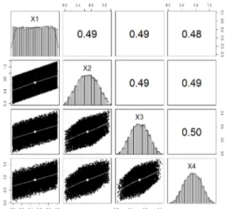
Although it would be tempting to follow the same general approach to construct a multivariate, non-normal distribution (i.e., select a covariance/correlation matrix, decompose it in its factors, BB0 and multiply
them times the matrix with uncorrelated, non-normal distributions of choice) and it has been done in the past (see, for instance, Hittner, May & Silver, 2003; Silver, Hittner & May, 2004; Wilcox & Tian Tian, 2008), it is of utmost importance to highlight that this proce-dure would only guarantee that the population corre-lation or covariance matrix is the one intended by the researcher. This property holds irrespective of whether the distributions to correlate are normal or non-normal. The univariate marginal distributions would lose their unique structures and, by the Central Limit Theorem, would become more and more normally distributed the more one-dimensional marginals are added. Figure 1 highlights this fact by reproducing the simulation condi-tions described in Silver, Hittner and May (2004) for the uniform case. Consider four independent,
identically-distributed random variables (X1, X2, X3, X4)which
fol-low a standard, uniform distribution, U(0, 1) and a pop-ulation correlation matrix R4×4 with equal correlations
of 0.5 in the off-diagonals. The process of multiply-ing the matrix with standard-uniform random variables times the Cholesky-decomposed R4×4to induce the
cor-relational structure (matrix B in the paragraph above)
ends up altering the univariate distributions such that they no longer follow the non-normal distributions in-tended by the researchers (Vale & Maurelli, 1983). The R code below exemplifies this process. In order to truly generate multivariate non-normal structures with a degree of control over the marginal distributions and the correlation structure simultaneously, more complex simulation techniques are needed.
# Block 1 set . seed (124)
## Creates the correlation matrix and factors it
R <- matrix ( rep (.5 ,16) ,4 ,4) diag (R) <- 1
C <- chol (R)
## Simulates independent Uniform random variables
x_1 <- runif (n = 10000 , min = 0, max = 1) x_2 <- runif (n = 10000 , min = 0, max = 1) x_3 <- runif (n = 10000 , min = 0, max = 1) x_4 <- runif (n = 10000 , min = 0, max = 1) X <- cbind (x_1 , x_2 , x_3 , x_4 )
## Post - multiplies the correlation - matrix factor to
## induce the correlation .
D <- X %*% C ## this is the 4- dimensional distribution
The NORTA family of methods
The NORmal To Anything (NORTA) family of meth-ods is a popular approach to generate multivariate, non-normal data within the social sciences. Although the ideas underlying this method can be traced back to Mar-dia (1970), Cario and Nelson (2007) were among the first ones to present this method in full generality and derive some of its fundamental theoretical properties. In essence, the NORTA method consists of three steps:
(1) Generate Z ∼ N(0d×1, Rd×d).
(2) Apply the probability integral transformation by using the multivariate normal cumulative
den-Figure 1. Four-dimensional distribution implied by the
simulation design of Silver, Hittner & May (2004) with assumed U(0, 1) marginal distributions
sity function (CDF) such that (Ui) = Φ(Zi) for
i= 1, 2, . . . , n.
(3) Choose a suitable inverse CDF, F−1(·), to
ap-ply to each marginal density of U so the the new multivariate random variable is defined as X= (F−1
1 (u1), F−12 (u2), ..., F−1d (ud))0. Notice that the
F−1
i (·)need not be the same for each i.
The NORTA algorithm encompasses a variety of methods where transformations of the one dimensional marginal distributions are applied to a multivariate nor-mal structure in an attempt to induce non-nornor-mality from the univariate to multivariate marginals.
Specific applications of the NORTA framework to sim-ulate non-normal data have different types of compu-tational limitations, depending on how the method is implemented. The first one can be found in Cario and Nelson (2007) Equation (1) which pertains to the way in which the correlation matrix of the distribution is as-sembled. Applying the transformations in Step 2 above will almost always end up changing the final value of the Pearson correlation between the marginal distribu-tions. Nevertheless, if Equation (1) in Cario and Nelson (2007) is solved for the correlation values intended for the researcher, then this correlation can be used in Step 1 above so that the final joint distribution has the popu-lation value originally desired. This approach, however, requires the correlation matrix to be created entry-by-entry. The estimation may result in a final correlation
matrix of the non-normal density which is not positive definite 1. Care needs to be taken when
implement-ing the NORTA approach to ensure both the non-normal and correlational structures are feasible.
The 3rdorder polynomial transformation
The 3rd order polynomial transformation, or the
Fleishman method, deserves a special mention because of the influence it has exerted on evaluating the robust-ness of statistical methods within psychology and the social sciences. Its original univariate characterization proposed by Fleishman (1978) and the multivariate ex-tension developed by Vale and Maurelli (1983) are, by far, the most widely used algorithms to evaluate viola-tions to the normality assumption in the social sciences. With upwards of 1100 citations combined between both articles, no other method to simulate non-normal data within these fields has been as extensively used as this approach.
The Fleishman method begins by defining a non-normal random variable as follows:
E= a + bZ + cZ2+ dZ3 (3)
where Z ∼ N(0, 1) and {a, b, c, d} are real-valued con-stants that act as polynomial coefficients to define the non-normally distributed variable E. The coefficients are obtained by finding the solution to the following system of equations: a+ c = 0 b2+ 6bd + 2c2+ 15d2= 1 (4) 2c(b2+ 24bd + 105d2+ 2) = γ1 24(bd+ c2[1+ b2+ 28bd]+ d2[12+ 48bd + 141c2+ 225d2])= γ2
where γ1is the population skewness and γ2is the
popu-lation excess kurtosis defined by the user. Fleishman-generated random variables are assumed to be stan-dardized (at least initially), so the mean is fixed at 0 and the variance is fixed at 1. By solving this system of equations, given the input of the user for (γ1, γ2), the
resulting polynomial coefficients can be plugged into Equation (3) so that the non-normal random variable Ehas its first four moments determined by the user.
As an example, pretend a user is interested in obtain-ing a distribution with a population skewness of 1 and a 1An n × n symmetric matrix A is said to be positive
defi-nite if for any real-valued vector vn×1, v>Av> 0. Equivalently,
all the eigenvalues of said matrix should be greater than 0. All covariance (and correlation) matrices are defined to be positive-definite. If they are not, they are not a true correla-tion/covariance matrix.
population excess kurtosis of 15. The following R code would generate the non-normal distribution E with the user-specified non-normality:
# Block 2 set . seed (124)
## Eqn4 ( the Fleishman system ) to be solved fleishman <- function (sk , krt ) {
fl_syst <- function ( skew , kurt , dd ) { b= dd [1 L ]; c= dd [2 L ]; d= dd [3 L ]; eqn1 = b ^2 + 6* b*d + 2* c ^2 + 15* d ^2 - 1 eqn2 = 2* c *( b ^2 + 24* b*d + 105* d ^2 + 2) - sk eqn3 = 24*( b*d + c ^2*(1 + b ^2 + 28* b*d) + d ^2*(12 + 48* b*d + 141* c ^2 + 225* d ^2) ) -krt
eqn <- c( eqn1 , eqn2 , eqn3 ) sum ( eqn * eqn )
}
sol <- nlminb ( start = c (0 ,0 ,1) , objective = fl_syst , skew = sk , kurt = krt )
}
## Solves the Fleishman system for skewness =1 , kurtosis =15
fleishman (1 ,15) $par
[1] 1.534711 0.170095 -0.306848
Although the original system contains four equations, notice that knowing c fully determines a (it simply switches sign). Once the polynomial coefficients are obtained, one simply needs to substitute them back in Equation (3): E= −0.170095 + 1.534711Z + 0.170095Z2−
0.306848Z3 Notice that, by construction, E is standard-ized, which can be seen in the system described in Equa-tion (4). Notice how the moments of E are the soluEqua-tions of the system, and the system has the first equation set to 0 (the mean of E) and the second equation set to 1 (the variance of E). The same values become negative in the R code to solve for the system.
Vale and Maurelli (1983) extended the Fleishman method by acknowledging the same limitation that was described in Section 2.2: If one Fleishman-transforms standard normal random variables and induces a cor-relation structure through a covariance matrix
decom-position approach (as described in Section 2.1), the resulting marginal distributions would no longer have the (γ1, γ2) values intended by the researcher. If, on
the other hand, one begins with multivariate normal data and then applies the Fleishman transformation to each marginal distribution, then the resulting correla-tion structure would not be the same as the one origi-nally intended by the researcher. Their solution, which is very much in line to the procedure described in Sec-tion 2.1, consisted of proposing a step between the final correlation structure and the 3rdorder polynomial
trans-formation called the “intermediate correlation matrix”. With this added step, one would simulate multivariate normal data where the intermediate correlation matrix holds in the population. Then one proceeds to apply the 3rd order polynomial transformation to each marginal
and, as they are transformed, the population correla-tions are altered to result in the final correlation matrix originally intended by the researcher. The intermediate correlation matrix is calculated as follows:
ρE1E2= ρZ1Z2(b1b2+ 3b1d2+ 3b2d1+ 9d1d2)+ ρ2
Z1Z2(2c1c2)+ ρ
3
Z1Z2(6d1d2) (5) where ρE1E2 is the intended correlation between the non-normal variables, {ai, bi, ci, di} are the polynomial
coefficients needed to implement the Fleishman trans-formation as described above and ρZ1Z2 is the interme-diate correlation coefficient. Solving for this correla-tion coefficient would give the user control over uni-variate skewness, excess kurtosis and the correlation/-covariance matrix.
The 3rdorder polynomial transformation proposed by
Fleishman (1978) (and extended by Vale and Maurelli (1983)) has several limitations. Tadikamalla (1980) and Headrick (2010) have commented on the fact that the combinations of skewness and excess kurtosis that can be simulated by this approach are limited when compared to other methods, such as the 5th order
poly-nomial transformation. The correlation matrix implied by Equation (5) is defined bivariately so that the inter-mediate correlation matrix has to be assembled one co-efficient at a time, increasing the probability that it may not be positive definite. The range of correlations that can be simulated is also restricted and contingent on the values of the intermediate correlation coefficients (Headrick, 2002). For instance, if one were to correlate a standard normal variable and a Fleishman-defined variable with (γ1 = 1, γ2 = 15), the researcher can only
choose correlations in the approximate [-0.614, 0.614] range. Correlations outside that range would make Equation (4) yield either non-real solutions or solutions outside [-1, 1] so that the correlation matrix becomes
unviable. If one were to continue with the example above, for the normal case it would imply that b1 = 1
and a1 = c1= d1= 0 such that E1= 0+(1)Z+(0)Z2+(0)Z3
and for E2 = −0.170095 + 1.534711Z + 0.170095Z2 −
0.306848Z3. Substituting these coefficients in Equation
(5) would yield: ρE1E2 = ρZ1Z2[(1)(1.534711)+ 3(1)(−0.306848) + 0 + 0]+ ρ2 Z1Z2(0)+ ρ 3 Z1Z2(0) ρE1E2 = ρZ1Z2(0.614167)
by setting ρZ1Z2 = ±1 one can see that the maximum possible correlation between the normal E1 and
non-normal E2 is 0.614167. For ρE1E2 to be greater than that, ρZ1Z2would have to be greater than 1, which would make the intermediate correlation matrix non-positive definite.
Although the previous limitations can be somewhat attenuated depending on the choice of γ1, γ2 and ρE1E2, there is one aspect of the Fleishman-Vale-Maurelli method that cannot be avoided because it is implicit within the theoretical framework in which it was de-veloped. The system described in Equation (4) and the intermediate correlation in Equation (5) are all poly-nomials of high degree. As such, they have multiple solutions and there is little indication as far as which solution should be preferred over others. Astivia and Zumbo (2018, 2019) have studied this issue before and documented the fact that the idiosyncrasies of the data generated by each solution can be as disparate as to al-ter the conclusions from previously published simula-tion studies. Although the 3rdorder polynomial method
has been used extensively to investigate the properties of statistical methods, more research is needed to un-derstand the properties and uses of the method itself to clarify to what extent the results from published sim-ulation studies are contingent on the type of data that can be generated through this particular method. For instance, would the results from previously-published simulation studies generalize if other data-generating algorithms were implemented? Can the data that ap-plied researchers collect be modelled through the 3rd
order polynomial method? Or does it follow other dis-tribution types? The 3rd order polynomial method
of-fers control over the first four moments of a distribution (mean, variance, skewness and kurtosis). Is this suffi-cient to characterize the data? Or would methods that allow control over even higher moments needed?
Copula distributions
Recently, copula distribution theory has begun to make an incursion into psychometric modelling and the behavioural sciences (e.g., Jones, Mair, Kuppens &
Weisz, 2019). Although the methods and techniques as-sociated with it are known within the fields of financial mathematics and actuarial science, the flexibility and power of this framework is becoming popularized in other areas to enhance the modelling of multivariate, non-normal data.
In its simplest conceptualization, a copula is a type of multivariate density where the marginal distributions are uniform and the dependence structure is specified through a copula function (Joe, 2014). Two important mathematical results power the flexibility of this the-oretical framework: the probability integral transform and Sklar’s theorem. The probability integral transform allows one to convert any random variable with a well-defined CDF into a uniformly distributed random vari-able (or vice-versa if there is an inverse CDF). Sklar’s theorem proves that any multivariate cumulative distri-bution function can be broken down into two indepen-dent parts: its unidimensional marginals and the copula function that relates them. Because of the generality of Sklar’s theorem, one can be guaranteed that, given some mild regularity conditions, (interested reader can consult Durante, Fernández-Sánchez & Sempi, 2013) for any multivariate distribution a copula function that parameterizes its joint CDF exists.
Introduction to Gaussian copulas
Gaussian copulas comprise perhaps the most com-monly used copula family for the analysis and simu-lation of data. They inherit many of the properties of the multivariate normal distribution that make them both analytically tractable and easy to interpret for re-searchers. In particular, Gaussian copulas rely on the covariance/correlation matrix to model the dependen-cies among its one-dimensional marginal distributions, so that the same covariance modelling that social scien-tists are familiar with generally translates into this type of copula modelling.
The Gaussian copula can be defined as follows: C(u1, u2, . . . , ud; Rd×d)= ΦRd×d(Φ
−1(u
1),Φ−1(u2), ...,Φ−1(ud))
(6) where ui, i = 1, 2, . . . , d are realizations of standard,
uniformly distributed random variables, Φ−1 is the
in-verse CDF of the univariate normal distribution, and ΦRd×d is the CDF for the d-variate Gaussian distribution with correlation matrix Rd×d. Similar to the NORTA
ap-proach, the process of building a Gaussian copula can be schematized in the following series of steps:
(1) Simulate from a multivariate normal distribution with desired correlation matrix.
(2) Apply the normal CDF to the newly-generated multivariate normal vector so that the columns
are now standard uniform bounded between 0 and 1.
(3) If the inverse CDF (the quantile function) of the desired non-normal distribution exist, apply said inverse CDF to each column of data. The resulting distribution would be a Gaussian copula with its one-dimensional marginal distributions selected by the researcher.
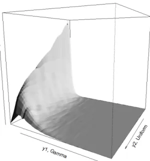
Let us assume a researcher wishes to simulate a bi-variate distribution (d = 2) where one marginal is y1 ∼ G(1, 1)and the other is y2 ∼ U(0, 1) with a
pop-ulation correlation ρ = 0.5. In the R programming lan-guage one could implement the following code so that the resulting Y is a simulated sample (n= 100, 000) from the Gaussian copula depicted in Figure 2 below.
# Block 3 set . seed (124) library ( mvtnorm )
## Simulates multivariate normal data rho <- .5
Z <- rmvnorm (n = 100000 , mean = c (0 ,0) , sigma = matrix (c(1 , rho , rho , 1) , 2, 2) ) ## Applies th normal CDF
U <- pnorm (Z)
## Quantile functions / inverse CDF for gamma ( y1 ) and uniform ( y2 ) marginals
y1 <- qgamma (U[, 1] , shape = 1, rate = 1) y2 <- qunif (U[, 2] , min = 0, max = 1) Y <- cbind (y1 , y2 )
## Correlation matrix of bivariate normal > cor (X)
[ ,1] [ ,2] [1 ,] 1.0000 0.5002 [2 ,] 0.5002 1.0000
## Correlation matrix of Gaussian copula > cor (Y)
y1 y2
y1 1.0000 0.4405 y2 0.4405 1.0000
Correlation shrinkage
Although the Gaussian copula induces a relation-ship between the Gamma and Uniform marginals, it is important to highlight that the original correlation of
Figure 2. Four-dimensional distribution implied by the
simulation design of Silver, Hittner & May (2004) with assumed U(0, 1) marginal distributions
ρ = 0.5 has now changed. When calculating the Pear-son correlation of the original sample from the bivari-ate normal distribution against the one from the Gaus-sian copula, the difference becomes apparent. There is a shrinkage of about 0.05-0.06 units in the correlation metric, with the shrinkage contingent on the the size of the initial correlation. Figure 32further clarifies this
issue by relating the initial correlation of the bivariate normal distribution to the final correlation of the Gaus-sian copula. In other words, there is a downward bias of approximately 0.15 units in the correlation metric for the theoretically maximum correlation of this copula. There are two important reasons for why this happens, even though it is not always acknowledged within the simulation literature in the social sciences.
First, both the probability integral transform
(U<-pnorm(Z)) and the quantile function (or inverse CDF) needed to obtain the non-normal marginal distri-butions (qgamma and qunif) are not linear transforma-tions. The Pearson correlation is only invariant under linear transformations so it stands to reason that if non-linear transformations are applied, there is no expec-tation that the correlation will remain the same. Sec-ond, there exists a result from copula distribution the-ory that places further restrictions on the range of the Pearson correlation referred to as the Fréchet–Hoeffding bounds. Hoeffding (1940) showed that the covariance 2Notice that Figure 3 is not directly related to the code in
Figure 3. Relationship between the original correlation
for the bivariate normal distribution and the final corre-lation for the Gaussian copula with G(1, 1) and U(0, 1) univariate marginals. The horizontal axis includes val-ues for the correlation for the bivariate normal distri-bution and the vertical axis presents the transformed correlation after the copula is constructed.The identity function (straight line) is included as reference.
between two random variables (S , T ) can be expressed as: Cov(S , T )= Z ∞ −∞ Z ∞ −∞ H(s, t) − F(s)G(t)dsdt (7) where H(s, t) is their joint cumulative distribution tion and F(s), G(t) are the marginal distribution func-tions of the random variables S and T respectively. De-fine H(s, t)min = max[F(s) + G(t) − 1, 0] and H(s, t)max =
min[F(s), G(t)]. Fréchet (1951) and Hoeffding (1940) independently proved that:
H(s, t)min≤ H(s, t) ≤ H(s, t)max (8)
and, by using these bounds in Equation (7) above, it can be shown that ρmin ≤ ρ ≤ ρmax, where ρ is the
linear correlation between the marginal distributions. The implication of this inequality is that, given the dis-tributional shape defined by F(s) and G(t), the corre-lation coefficient may not fully span the [-1, 1] theo-retical range. For instance, Astivia and Zumbo (2017) have shown that for the case of standard, lognormal variables the theoretical correlation range is restricted to [−1/e, 1] (approximately [−0.368, 1]), where e is the base of the natural logarithm. For the Gaussian cop-ula above, the theoretical upper bound is approximately
0.85 on the positive side of the correlation range. When the inverse CDFs are implemented to generate the non-normal marginals, the Fréchet–Hoeffding bounds are induced, restricting the types of correlational structures that multivariate, non-normal distributions can gener-ate when compared to multivarigener-ate normal ones. More-over, the Fréchet–Hoeffding bounds are the greatest lower and least upper bounds. That is, the Fréchet– Hoeffding bounds cannot be improved upon in general (Joe, 2014; Nelsen, 2010). Although there is nothing that can expand the Fréchet–Hoeffding bounds to the full [-1, 1] range if the marginals are fixed, the interme-diate correlation matrix approach described in Section 2.2 can be used to find the proper value for the corre-lation coefficient needed to initialize the Gaussian cop-ula, if a specific population value is desired. As long as the value on this intermediate correlation is within the bounds specified by the non-normal marginals, the final correlation after the marginal transformation is com-pleted will match the population parameter intended by the researcher.
Relationship of the NORTA method, the Vale– Maurelli algorithm and Gaussian copulas. Gaussian copulas have other important connections to the sim-ulation work done within the social sciences, notably, the fact that the NORTA method can be parameterized as a Gaussian copula (Qing, 2017). By extension, the Vale–Maurelli algorithm has also been proved to be a special case of Gaussian copulas so that the majority of simulation work conducted in the social sciences has re-ally only considered the Gaussian copula as its test case (Foldnes & Grønneberg, 2015; Grønneberg & Foldnes, 2019). The same issues and limitations presented in Sections 2.2 and 2.3 are, in fact, exchangeable given that the data-generating methods considered in both cases share the same essential properties.
Distributions closed under linear transformation and their connection to simulating multivariate, non-normality
As presented in Section 2.1, one of the many attrac-tive properties of the normal distribution is that the sum of independent, normal random variables is itself normally distributed. This property is known as being “closed under convolutions” (i.e., when one combines in a certain way or “convolves” random variables, the resulting random variable belongs to the same family as its original components. Through the use of this prop-erty, one can define the multivariate normal distribu-tion by finding linear combinadistribu-tions (i.e., convoludistribu-tions) of the one-dimensional normal marginals that will re-sult in Xn×d ∼ N (µµµd×1, ΣΣΣd×d). Although not very
probabil-ity distributions, making it the preferred starting point to defining multivariate generalizations of them. Con-tinuous distributions such as the Cauchy and Gamma share this property and their multivariate extensions de-pend on it. The Gamma distribution is a particularly relevant case given its connection to other well-known probability distributions such as the exponential and the chi-square. If X1 ∼ G(α1, β) and X2 ∼ G(α2, β) then
X1+ X2 ∼ G(α1 + α2, β). Notice how the property of
closeness is only true the rate parameter β is the same. The sum of two generic gamma distributions is not nec-essarily gamma-distributed (see Moschopoulos, 1985). For the interested reader, an introduction to the theory of gamma distributions can be found in Chapter 15 of Krishnamoorthy (2016).
As a motivating example to showcase a multivari-ate distribution that is not Gaussian, yet closed un-der convolutions, consiun-der P and Q to be indepen-dently distributed Poisson random variables with pa-rameters (λP, λQ) respectively. If W = P + Q then
W ∼ Poisson(λW = λP + λQ). By using this property,
one can generalize the univariate Poisson distribution to multivariate spaces. Consider P, Q and V to be in-dependent, Poisson distributed random variables with respective parameters λP, λQ and λV. Define two new
random variables P∗and Q∗as follows:
P∗= P + V
Q∗= Q + V (9)
Because P∗ and Q∗ share V in common, (P∗, Q∗)0
ex-hibits Poisson-distributed, univariate marginal distribu-tions with a covariance equal to λV. Notice that this
construction only allows for the case where the covari-ance between P∗ and Q∗ is positive because, by
defini-tion, the parameter λ of a Poisson distribution must be positive. Figure 4 shows the bivariate histogram of a simulated example with P ∼ Poisson(1), Q ∼ Poisson(2) and V ∼ Poisson(3). In R code:
# Block 4 set . seed (124)
## Simulates independent Poisson random variables
P <- rpois (100000 , lambda = 1) Q <- rpois (100000 , lambda = 1) V <- rpois (100000 , lambda = 3)
## Creates joint distribution with marginal Poisson random variables
Pstar <- P + V Qstar <- Q + V cov ( Pstar , Qstar ) [1] 2.969006
Figure 4. Bivariate Poisson distribution with
Cov(P∗, Q∗)= λ V = 3.
With the exception of the multivariate normal distri-bution, relying on the property of being closed under convolutions is not a widely used method to simulate non-normal data for the social sciences. Very few distri-butions have this property and, even among those that do, there may be further restrictions in place that limit either the type of distributions that can be generated or the dependency structures that can be modelled (Flo-rescu, 2014). As shown in the example above, although one could use this method recursively to generate a mul-tivariate Poisson distribution with a pre-specified ance matrix, one is restricted to only positive covari-ances, given the limitation that all λ parameters must be positive. In spite of the lack of attention given to this simulation approach, the present section is intended to remind the reader that the properties of univariate dis-tributions rarely generalize to multivariate spaces un-altered. If approaches similar to this are used without showing closedness under convolutions first, there will be a discrepancy between the simulation design and the actual implementation of the simulation method so that one can no longer be sure which exact distributions are being generated.
Alternative Approaches
There exist a variety of alternative approaches that were not considered in this overview but which are quickly gaining use and prominence within the
simula-tion literature in the social sciences. Although not all of these methods share a common theoretical frame-work and the details of many of them are beyond the scope of the present manuscript, there is relevance in mentioning them for the interested reader. Particularly because they can be used to explore simulation condi-tions beyond the skewness and kurtosis of the univariate distributions, which is the general approach that per-meate the simulation literature in the social sciences. Grønneberg and Foldnes (2017) and Mair, Satorra and Bentler (2012) have extended the copula distribution approaches beyond the Gaussian copula to help cre-ate more flexible, non-normal structures that induce different types of non-normalities, such as tail depen-dence or multivariate skew. Qu, Liu and Zhang (2019) have recently extended the Fleishman approach to mul-tivariate higher moments and, to this day, it is one of the few methods available that allow researchers to set population values of Mardia’s multivariate skew-ness and kurtosis, which allows researchers a certain degree of control over both univariate and multivari-ate non-normality. Ruscio and Kaczetow (2008) de-veloped a sampling-and-iterate algorithm that allows one to simulate from any arbitrary number of distribu-tions while keeping control of the correlational
struc-ture. Although not much is known about the
theo-retical properties of this method, it offers the advan-tage of allowing users to induce any level of correla-tion to an empirical datasets that they may have col-lected. Therefore, the user is given a choice to either simulate from theoretical distributions or from a par-ticular dataset of interest. Auerswald and Moshagen (2015) as well as Mattson (1997) have considered the problem by restating it under a latent variable frame-work and inducing the non-normality through the la-tent variables. Methods like this would allow the users to more accurately control the distributional assump-tions of latent variables, which could be of interest to researchers in Structural Equation Modelling or Item Response Theory. The work of Kowalchuk and Headrick (2010), Pant and Headrick (2013) and Koran, Headrick and Kuo (2015) has extended the properties of univari-ate, non-normal distributions such as the g-and-h fam-ily of distributions or the Burr famfam-ily of distributions to multivariate spaces, in an attempt to allow researchers the flexibility to select from a wider collection of non-normal structures. These methods share some similari-ties with the NORTA approaches in terms of generating multivariate non-normal data by manipulating the uni-dimensional marginals of the joint distribution. Never-theless, most of this work uses L−moments as the coeffi-cients that control the non-normality of the data, not the conventional 3rdand 4thorder moments (i.e., skewness
and kurtosis) familiar to most researchers. The creators of these methods offer readily-available software imple-mentations of them, although not all are available in the same programming languages.
In spite of these modern advances, the NORTA ap-proaches in general (and the 3rdorder polynomial
trans-formation in particular) have dominated the robustness literature in simulation studies within psychology and the social sciences. As such, I present three recommen-dations that I believe would aid in the design, planning and reporting of simulation studies:
Recommendations for the use of the 3rdorder
polynomial method
If the Fleishman (1978) method (for the univariate case) or the Vale and Maurelli (1983) multivariate ex-tension are used in simulations, it would be beneficial to report both the transformation coefficients, {a, b, c, d} in Equation (4), and the intermediate correlation ma-trix assembled from Equation (5). For instance, Astivia and Zumbo (2015) conjectured and Foldnes and Grøn-neberg (2017) proved that the asymptotic covariance matrix used in the robust corrections to non-normality within SEM depends on these polynomial coefficients and the intermediate correlation matrix. Different sets of solutions create different asymptotic covariance ma-trices so that small-sample recommendations that use this simulation technique may be highly contingent on the type of data that could be generated through this ap-proach. By reporting which coefficients were used, one can at least provide a clearer, more reproducible simu-lation for other researchers to interpret. For a concrete example, please see Sheng and Sheng (2012)’s “Study Design” section where the polynomial coefficients for each type of non-normality are listed.
General Recommendations
Accounting for different types of multivariate non-normality
Since there is an infinite way for multivariate distri-butions to deviate from the normality assumption (yet there is only one way for data to be multivariate nor-mal), attempting different simulation methods may of-fer a more comprehensive view of what type of ro-bustness properties the methods under investigation are sensitive to. Consider, for instance, Falk’s (2018) sim-ulation study investigating the performance of robust corrections to constructing confidence intervals within SEM. Three data-generating mechanisms were used for non-normal data: the Vale–Maurelli approach, contam-inated normal and a Gumbel copula distribution. The contaminated normal and the Gumbel copula case had
univariate distributions which were very close to the normal, yet the coverage for the confidence intervals was very poor, bringing into question recommendations (such as those in Finney & DeStefano, 2006) who argue that robust corrections for SEM models should be used based on the distributions of the indicators. Although the previous recommendations make sense in light of previous simulation work (which relied almost entirely on the 3rdorder polynomial approach) the results found
in Falk (2018) help highlight that non-normalities in higher dimensions can still impact data analysis, even if researchers are unaware of these properties.
Justify and tailor your type of non-normality
It is crucial for methodologists and quantitative social scientists to be able to tailor their simulation results to the kind of scientific audience and research field they wish to inform. One of the main objections to any simu-lation study is its generalizability and how the findings presented and recommendations offered would fare if the simulation conditions were altered. As it stands today, whenever a simulation study exploring the is-sue of non-normality is conducted, the simulation de-sign is usually informed by previous simulations and, for lack of a better term, “tradition”. Take, for instance, the population values of skewness and excess kurtosis γ1 = 2, γ2 = 7 to denote “moderate” non-normality and
γ1 = 3, γ2 = 21 for “extreme” non-normality. These
val-ues were originally used in Curran, West and Finch’s (1996) simulation study on the influence that non-normality exerts on the chi-squared test of fit for SEM. Since then, these (γ1, γ2) (absolute) values, have
ap-peared in Berkovits, Hancock and Nevitt (2000); Lodder et al., (2019); Nevitt and Hancock, (2000); Shin, No and Hong, (2019); Tofighi and Kelley, (2019) Vallejo, Gras and Garcia, (2007) and more. The fact of the mat-ter is, however, that we do not know if these values (or the Gaussian copula implied by the Vale–Maurelli ap-proach) are representative of the type of data encoun-tered in psychology and other social sciences. And with the exception of Cain, Zhang & Yuan (2017), there has not been much interest within the published literature in documenting both the type of univariate and mul-tivariate distributions that are commonly found in our areas of research. At this point in time, I would argue that we, as methodologists, do not have a good sense of whether the type of data we simulate in our studies is reflective of the type of data that exists in the real world. An important solution to address this problem is the movement towards open science, reproduciblity and open data. Having access to raw data grants methodolo-gists and quantitative researchers the ability to actually mimic the idiosyncrasies that applied researchers face
every day and offer recommendations that address them directly. Becoming familiar with alternative modes of data-simulation would also help improve the general-izability of simulation results. As commented on Sec-tion 2.2.1, the 3rd order polynomial approach to
non-normal simulation enjoys a considerable predilection amongst quantitative researchers, to the detriment of other approaches. Considering even just one other gorithm when conducting simulations would help al-leviate this limitation and encompass a wider class of non-normalities than what one can find the the 3rd
or-der polynomial method. Finally, quantitative method-ologists may benefit from using population parameters found in the literature. Relying on previously-published simulations to choose effect sizes is the current, “stan-dard” which may limit recommendations that do not necessarily match different areas of research. If one sim-ulates something it should at least attempt to emulate real life, not other simulations.
The meta-scientific investigation of simulation stud-ies
The goal of a considerable amount of simulation re-search in the social sciences is to provide guidelines and best practice recommendations for data analysis under violation of distributional assumptions. Because of this, it is of utmost importance that applied researchers also become familiar (to a certain degree) with how quanti-tative methodologists conduct their research to be able to understand whether or not their recommendations are relevant to the analyses they may conduct. Ideally, if an applied researcher is unfamiliar with the method-ological literature yet looks for a better understanding of how simulation results may aid in their analyses, they should consider consulting with a quantitative expert. Much like in the case of applied research, every simula-tion study can have their own idiosyncrasies and design peculiarities that require a more nuanced understand-ing of what the original authors presented, and spot-ting potential gaps on a simulation design usually re-quires a certain degree of mathematical sophistication that, although desirable, is not usually a required skill amongst applied researchers. Perhaps the easiest way in which these issues can be conceptualized for applied researchers is by considering simulation studies as the analog of empirical, experimental work as opposed to formal mathematical argumentation.
Although simulation studies would ideally go hand-in-hand with the statistical and mathematical theory that lends legitimacy to their results, enough examples and case studies have been provided in the previous sections of this article to highlight the fact that this is not often the case. Just as “methods effects” can
intro-duce unnecessary noise and uncertainty when conduct-ing experiments, operatconduct-ing from a “black box” perspec-tive when conducting simulation studies can also create a disconnection between the theory and the design of a simulation study. The fact of the matter is that al-most no research exists that attempts to analyze and validate the current practices of computer simulation studies. Whereas the movement towards open, repro-ducible science has yielded important insights into ques-tionable research practices like p-hacking or researcher degrees of freedom, quantitative fields have remained virtually unexplored, due perhaps to their technical na-ture and the fact that a more solid theoretical founda-tion in statistics is needed in order to recognize the is-sues presented. A meta-scientific study of the theory and practice of simulation studies is desperately needed in order to begin to understand the types of questions and answers that are presented within the quantitative fields of the social sciences. It is my sincere hope that by offering this overview, researchers can begin to famil-iarize themselves with some of the methodological and epistemological issues that computer simulations pose and open a dialogue between methodological and ap-plied researchers in an area that is usually restricted to the most technically-minded amongst us.
Author Contact
Dr. Oscar L. Olvera Astivia. oastivia@uw.edu
ORCID 0000-0002-5744-2403
Conflict of Interest and Funding
No conflict of interest and no external funding.
Author Contributions
Dr. Astivia is the solo author of this article. He was in charge of conceptualization, analysis, software coding as well as the write-up and revisions.
Acknowledgements
I would like to thank the editor-in-chief, Dr. Rickard Carlsson and my action editor Dr. Daniël Lakens for their incredible help and support during the review pro-cess of this manuscript. I would also like to extend my sincere thanks to my wonderful reviewers Wen Qu, Anna Lohman and Dr. Steffen Grønneberg for the time and effort they spent to help improve this manuscript. Last but not least, I would like to also thank my col-league and dear friend Dr. Edward Kroc whose stimu-lating conversations always provide me with insights I could not have achieved by myself.
Open Science Practices
This article earned Open Materials badge for making the materials openly available. In this case, the material is the code that is presented inline. It has been verified that the analysis reproduced the results presented in the article. The entire editorial process, including the open reviews, are published in the online supplement.
References
Astivia, O.L.O. & Zumbo, B. D. (2017). Population mod-els and simulation methods: the case of the Spear-man rank correlation. British Journal of
Mathemat-ical and StatistMathemat-ical Psychology, 70, 347-367. doi:
10.1111/bmsp.12085
Astivia, O.L.O. & Zumbo, B. D. (2018). On the solution multiplicity of the Fleishman method and its impact in simulation studies. British Journal of
Mathemat-ical and StatistMathemat-ical Psychology, 71, 437-458. doi:
Astivia, O.L.O., & Zumbo, B. D. (2019). A Note on the solution multiplicity of the Vale–Maurelli in-termediate correlation equation. Journal of
Educa-tional and Behavioral Statistics, 44, 127-143. doi:
10.3102/1076998618803381
Auerswald, M. & Moshagen, M. (2015). Generat-ing correlated, non-normally distributed data usGenerat-ing a non-linear structural model.Psychometrika, 80, 920-937. doi: 10.1007/s11336-015-9468-7 Beasley, T. M. & Zumbo, B. D. (2003). Comparison of
aligned Friedman rank and parametric methods for testing interactions in split-plot designs.
Compu-tational Statistics and Data Analysis, 42, 569–593.
doi: 10.1016/S0167-9473(02)00147-0
Beisbart, C. & Norton, J. D. (2012). Why Monte Carlo simulations are inferences and not experiments.
In-ternational Studies in the Philosophy of Science, 26,
403-422. doi: 10.1080/02698595.2012.748497 Cain, M. K., Zhang, Z. & Yuan, K. H. (2017). Univariate
and multivariate skewness and kurtosis for mea-suring non-normality: Prevalence, influence and estimation. Behavior Research Methods, 49, 1716-1735. doi: 10.3758/s13428-016-0814-1
Cario, M. C. & Nelson, B. L. (1997). Modeling and gen-erating random vectors with arbitrary marginal dis-tributions and correlation matrix (pp. 1-19).
Tech-nical Report, Department of Industrial Engineering and Management Sciences, Northwestern University.
Evanston, Illinois.
Carsey, T. M. & Harden, J. J. (2013). Monte Carlo
Sim-ulation and Resampling Methods for Social Science.
Sage Publications.
Curran, P. J., West, S. G. & Finch, J. F. (1996). The robustness of test statistics to non-normality and specification error in confirmatory factor
anal-ysis. Psychological Methods, 1, 16–29. doi:
10.1037/1082-989X.1.1.16
Durante F., Fernández-Sánchez, J. & Sempi, C. (2013) How to Prove Sklar’s Theorem. In Bustince H., Fer-nandez J., Mesiar R., Calvo T. (eds) Aggregation
Functions in Theory and in Practise. Advances in In-telligent Systems and Computing, vol 228. Springer,
Berlin, Heidelberg
Falk, C. F. (2018). Are robust standard errors the best approach for interval estimation with non-normal data in structural equation modeling? Structural
Equation Modeling: A Multidisciplinary Journal, 25,
244-266. doi: 10.1080/10705511.2017.1367254
Finch, H. (2005). Comparison of the performance
of non-parametric and parametric MANOVA test statistics when assumptions are violated.
Method-ology, 1, 27–38. doi: 10.1027/1614-1881.1.1.27
Fleishman, A. I. (1978). A method for simulating
non-normal distributions. Psychometrika, 43, 521-532. doi: 10.1007/BF02293811
Florescu, I. (2014). Probability and Stochastic Processes. John Wiley & Sons
Foldnes, N. & Grønneberg, S. (2015). How general is the Vale–Maurelli simulation approach?.
Psychome-trika, 80, 1066-1083. doi:
10.1007/s11336-014-9414-0
Fréchet, M. (1951). Sur les tableaux de corrélation dont les marges sont donnés. Annales de l’Université
de Lyon Section A:Sciences mathématiques et as-tronomie, 14, 53-77.
Grønneberg, S. & Foldnes, N. (2017). Covariance model simulation using regular vines. Psychometrika, 82, 1035-1051. doi: 10.1007/s11336-017-9569-6 Grønneberg, S. & Foldnes, N. (2019). A Problem with
discretizing Vale–Maurelli in simulation studies.
Psychometrika, 84, 554-561. doi:
10.1007/s11336-019-09663-8
Headrick, T. C. (2002). Fast fifth-order polynomial transforms for generating univariate and multi-variate non-normal distributions. Computational
Statistics and Data Analysis, 40, 685-711. doi:
10.1016/S0167-9473(02)00072-5
Headrick, T. C. (2010). Statistical Simulation: Power
Method Polynomials and Other Transformations.
Chapman & Hall/CRC.
Hess, B., Olejnik, S. & Huberty, C. J. (2001). The ef-ficacy of two improvement-over-chance effect sizes for two group univariate comparisons under vari-ance heterogeneity and nonnormality. Educational
and Psychological Measurement, 61, 909–936. doi:
10.1177/00131640121971572
Hittner, J. B., May, K. & Silver, N. C. (2003). A Monte Carlo evaluation of tests for comparing dependent correlations. The Journal of General Psychology, 130, 149-168. doi: 10.1080/00221300309601282
Hoeffding, W. (1940). Scale-invariant correlation the-ory. In Fisher, N.I. & Sen, P.K. (Eds.) The Collected
Works of Wassily Hoeffding (pp. 57-107). Springer,
New York, NY.
Hoover, W.G. & Hoover, C.G. (2015). Simulation and
Control of Chaotic Non-equilibrium Systems. World
Scientific.
Joe, H. (2014). Dependence modeling with copulas. New York, NY: Chapman and Hall/CRC.
Jones, P. J., Mair, P., Kuppens, S. & Weisz, J.
R. (2019, March 28). An Upper Limit to
Youth Psychotherapy Benefit? A Meta-Analytic
Copula Approach to Psychotherapy Outcomes. https://doi.org/10.31219/osf.io/jsmf5
Koran, J. Headrick, T. C. & Kuo, T. C. (2015). Simulat-ing univariate and multivariate non-normal
distri-butions through the method of percentiles.
Mul-tivariate Behavioral Research, 50, 216-232. doi:
10.1080/00273171.2014.963194
Kotz, S., Balakrishnan, N. & Johnson, N. L. (2004).
Con-tinuous Multivariate Distributions, Volume 1: Mod-els and applications. (Vol. 1). John Wiley & Sons.
Kowalchuk, R. K. & Headrick, T. C. (2010). Simulat-ing multivariate g-and-h distributions. British
Jour-nal of Mathematical and Statistical Psychology, 63,
63–74. doi: 10.1348/000711009X423067
Krishnamoorthy, K. (2016). Handbook of
Statisti-cal Distributions with Applications. New York, NY:Chapman and Hall/CRC.
Mair, P., Satorra, A. & Bentler, P. M. (2012). Generating non-normal multivariate data
us-ing copulas: Applications to SEM.
Multivari-ate Behavioral Research, 47, 547-565. doi:
10.1080/00273171.2012.692629
Mardia, K. V. (1970). A translation family of bivariate distributions and Fré chet’s bounds. Sankhya: The Indian Journal of Statistics, Series A. 119-122. doi: jstor.org/stable/25049643
Mattson, S. (1997). How to generate non-normal data for simulation of structural equation models.
Mul-tivariate Behavioral Research, 32, 355-373. doi:
10.1207/s15327906mbr3204_3
Moschopoulos, P. G. (1985). The distribution of the sum of independent gamma random variables. Annals of
the Institute of Statistical Mathematics, 37, 541-544.
doi: 10.1007/bf02481123
Nelsen, R. B. (2010). An Introduction to Copulas.
Springer Science & Business Media.
Oshima, T. C. & Algina, J. (1992). Type I error rates for James’s second-order test and Wilcox’s Hm test under heteroscedasticity and non-normality.
British Journal of Mathematical and Statistical
Psy-chology, 45, 255-263. doi:
10.1111/j.2044-8317.1992.tb00991.x
Pant, M. D. & Headrick, T. C. (2013). A method for simulating Burr Type III and Type XII distributions through moments and correlations. ISRN Applied
Mathematics. doi: 10.1155/2013/191604
Qing, X. (2017). Generating correlated random vec-tor involving discrete variables. Communications in
Statistics - Theory and Methods, 46, 1594-1605. doi:
10.1080/03610926.2015.1024860
Qu, W., Liu, H. & Zhang, Z. (2019). A method of generating multivariate non-normal random num-bers with desired multivariate skewness and
kur-tosis. Behavior Research Methods, 1-8. doi:
10.3758/s13428-019-01291-5
Ruscio, J. & Kaczetow, W. (2008). Simulating multivari-ate non-normal data using an iterative algorithm.
Multivariate Behavioral Research, 43, 355-381. doi:
10.1080/00273170802285693
Sheng, Y. & Sheng, Z. (2012). Is coefficient alpha robust to non-normal data? Frontiers in Psychology, 3, 1-13. doi: 10.3389/fpsyg.2012.00034
Shieh, Y. (April, 2000). The Effects of Distributional Characteristics on Multi-Level Modeling Parameter Estimates and Type I Error Control of Parameter Tests under Conditions Of Non-Normality. Paper
presented at the annual meeting of the American Ed-ucational Research Association, New Orleans.
Silver, N. C., Hittner, J. B. & May, K. (2004). Test-ing dependent correlations with non-overlappTest-ing variables: a Monte Carlo simulation. The
Jour-nal of Experimental Education, 73, 53-69. doi:
10.3200/JEXE.71.1.53-70
Vale, C. D. & Maurelli, V. A. (1983). Simulating mul-tivariate non-normal distributions. Psychometrika,
48, 465-471. doi: 10.1007/BF02293687
Tadikamalla, P. R. (1980). On simulating non-normal distributions. Psychometrika, 45, 273-279. doi: 10.1007/BF02294081
Wiedermann, W. T. & Alexandrowicz, R. W. (2007). A plea for more general tests than those for location only: Further considerations on Rasch & Guiard’s’ The robustness of parametric statistical methods’.
Psychology Science, 49, 2-12. doi:
10.1007/978-94-009-6528-7_24
Wilcox, R. R. & Tian, T. (2008). Comparing depen-dent correlations. The Journal of General
Psychol-ogy, 135, 105-112. doi:
10.3200/GENP.135.1.105-112
Zimmerman, D. W. & Zumbo, B. D. (1990). The relative power of the Wilcoxon-Mann-Whitney test and Stu-dent t test under simple bounded transformations.
The Journal of General Psychology, 117, 425-436.
Appendix
###### FIGURE 1 ################### library ( psych )
pairs . panels (D , hist . col = " grey ", rug = F , col . smooth = " white ") #####################################################
###### FIGURE 2 ################### library ( rgl )
library ( MASS )
bivn <- cbind (y2 , y1 )
X <- kde2d ( bivn [, 1] , bivn [, 2] , n = 50)
persp (X , phi = 10 , theta = 120 , shade = 1, border = NA , xlab = c (" y2 , Uniform ") , ylab = c (" y1 , Gamma ") , zlab = c ("") ) ##################################################### ###### FIGURE 3 ################### library ( mvtnorm ) library ( ggplot2 ) r <- seq ( from = 0, to = .99 , by = .01) rr <- double (100) for (i in 1:100) {
X <- rmvnorm (n = 100000 , mean = c (0 ,0) , sigma = matrix (c(1 , r[i], r[i], 1) , 2, 2) ) U <- pnorm (X)
y1 <- qgamma (U[, 1] , shape = 1, rate = 1) y2 <- qunif (U[, 2] , min = 0, max = 1) rr [i] <- cor (y1 , y2 )
}
dat <- data . frame ( cbind (r , rr )) fun .1 <- function (x)x
p1 <- ggplot (dat , aes (r , rr )) + geom_point ( colour = " black ") + stat_function ( fun = fun .1) p1 + theme_bw () + scale_x_continuous ( breaks = seq (0 , 1, by = .1) ) +
scale_y_continuous ( breaks = seq (0 , 1, by = .1) ) + xlab (" Bivariate normal correlation ") + ylab (" Gaussian copula correlation ") + ggtitle (" Gaussian copula correlation against bivariate normal correlation ") + theme ( plot . title = element_text ( hjust = 0.5) ) #####################################################
###### FIGURE 4 ################### set . seed (124)
library ( plot3D )
Y <- rpois (100000 , lambda =1) Z <- rpois (100000 , lambda =3) Xstar <- X + Z
Ystar <- Y + Z
z <- table ( Xstar , Ystar )
## Plot as a 3D histogram :
hist3D (z=z , phi =10 , xlab =c (" P ") , ylab =(" Q ") , zlab =c ("") , theta = -120 , col = ramp . col (c (" white ", " black ") ) , border = " black ", colkey = FALSE )