2016, 2(1–2)
Published by the Scandinavian Society for Person-Oriented Research Freely available at
http://www.person-research.org
DOI: 10.17505/jpor.2016.08Performing Cluster Analysis Within a Person-Oriented Context:
Some Methods for Evaluating the Quality of Cluster Solutions
András Vargha
1, Lars R. Bergman
2, Szabolcs Takács
1 1Károli Gáspár University, Budapest2Stockholm University, Stockholm
Contact
vargha.andras@kre.hu
How to cite this article
Vargha, A., Bergman, L. R., & Takács, S. (2016). Performing Cluster Analysis Within a Person-Oriented Context: Some Methods for Evaluating the Quality of Cluster Solutions. Journal of Person-Oriented Research, 2(1–2), 78–86. DOI: 10.17505/jpor.2016.08
Abstract: The paper focuses on the internal validity of clustering solutions. The “goodness” of a cluster structure can be
judged by means of different cluster quality coefficient (QC) measures, such as the percentage of explained variance, the point-biserial correlation, the Silhouette coefficient, etc. The paper presents the most commonly used QCs occurring in well-known statistical program packages, and we have strived to make the presentation as non technical as possible to make it accessible to the applied researcher. The focus is on QCs useful in person-oriented research. Based on simulated data with independent variables, the paper shows that QCs can be strongly influenced by the number of clusters and the number of input variables, and that the value of a QC can be fairly high even in the absence of any real cluster structure. When evaluating the internal validity, it is helpful to relate the QCs of a clustering solution to those obtained in parallel analyses of random data. We also introduce a new type of QC, measuring the relative improvement (MORI) of a QC obtained for a certain clustering solution relative to the corresponding QC based on a relevant type of random data.
Keywords: person-oriented methods, classification, internal validity, cluster amalysis, cluster quality coefficients, MORI, relative improvement, ROPstat
Introduction
For thousands of years, man has been engaged in creating classificatory systems. These have, for instance, concerned physical objects, celestial phenomena, tribe identification, dividing tribe members into good or bad hunters, into good or bad food preparers, etc. In fact, we are hard-wired to cre-ate order out of chaos by classification. This way of think-ing, natural to us, was extensively used by early scientists, like the Greek philosophers, and also much used in psychol-ogy and psychiatry up to the beginning of the 20thcentury, and in biology and medicine a classificatory approach is still much in use. However, in psychology it largely fell into dis-repute and it has since many decades been replaced by a dimensional approach. One reason for this was the
subjec-tivity involved in early classificatory approaches and its fre-quent view of class membership as innate and unalterable; characteristics that do not apply to modern classificatory research.
In this article, our attention will be restricted to classi-fication analysis performed using cluster analysis (CA) of a sample of persons, based on information of their val-ues in a set of continuous variables (the value profile /pat-tern). The purpose is to obtain a clustering solution (a set of classes of persons) where each cluster is as homogeneous as possible (persons in the same cluster have similar value profiles) and distinct (persons from different clusters have different value profiles). To achieve this, a large number of clustering algorithms exist that, partly independently, have been developed in many sciences, foremost in
biol-ogy and computer science but also in psycholbiol-ogy. It should be recognized that different clustering methods normally do not produce identical clustering solutions, even for a given number of clusters, although good algorithms tend to produce similar findings. It should also be recognized that finding the “true” number of clusters is normally not possible by objective means. This is not surprising, consid-ering the complexity of modeling observations in a high di-mensional space, often with substantial errors of measure-ment present, and also considering that in the general case there is no help from a theory providing specifications and assumptions that can be used in the search of an optimal method.
It is the purpose of this article to suggest and exemplify suitable methods for evaluating the internal validity of a clustering solution. This is not done in a general sense but within the framework of a person-oriented approach, which provides a theoretical background and assumptions that may simplify the task of finding a good clustering pro-cedure. The framework and its implications for the choice of clustering method are discussed below. However, before that is done it is helpful to first introduce CA and what we mean by quality coefficients.
Cluster Analysis and Quality
Coeffi-cients
CA, technically, is a statistical method where the aim is to create groups of objects (clusters) such that the objects in a cluster will be similar (or related) to one another and different (unrelated) from objects belonging to other clus-ters (Pardo,2010). Each type of CA attempts to reach this aim by using an algorithm optimizing some criterion. Hav-ing obtained a cluster structure, it is important to know how “good” it is. Is it better than the structure obtained by another procedure, for instance using a different CA al-gorithm, another measure of (dis)similarity, or using a dif-ferent number of variables or clusters? Is it better than a structure obtained from a random data set? To help in an-swering these types of questions there are special measures, the so called clustering quality coefficients (QCs), by means of which the goodness of a cluster model can be evaluated. The term validation is used here to refer to the evaluation process of a cluster structure. By “internal validation” we mean a cluster validation where only internal criteria are used to evaluate a cluster structure, based solely on the in-formation intrinsic to the data alone (Rendón, Abundez, Arizmendi, & Quiroz,2011).
In the large literature of classifications many QCs have been introduced (see e.g.Desgraupes,2013, where 43 QCs are explained, andRendón et al.,2011). However, the most common statistical program packages (e.g. SPSS or SAS) provide only few of them, if any. Exceptions are ROPstat (see
www.ropstat.com
or Vargha, Torma, & Bergman, 2015) with its pattern-oriented module, providing 7 QCs, and the “clValid” module in the R package, providing more than 40 QCs (Desgraupes,2015) for evaluating the internal validity of a cluster model.Different QCs focus on different aspects of a cluster struc-ture, thus it is very important to choose an appropriate set of QCs to evaluate a concrete model. In general, QCs try to measure one or both of two main characteristics of a cluster structure, namely compactness (cohesion) and separabil-ity (Jegatha Deborah, Baskaran, & Kannan, 2010;Pardo, 2010; Rendón et al., 2011). A structure is compact if it consists of homogeneous clusters, where the within-cluster variability is low. The separability of a structure concerns the degree to which the clusters are different from each other. From the many QCs we identify the following four types (note that some QCs do not solely belong to any of the types).
(A) Cohesion indices. Some QCs (indices Ball-Hall, Banfeld-Raftery, Calinski-Harabasz, etc., see Desgraupes, 2013; or HCmean = average cluster homogeneity, see Vargha et al., 2015) depend only on within-cluster distances: the higher the cohesion, the better the structure. Also EESS% (= explained error sum of squares percentage) is a cohesion type QC, in spite of the fact that the total sum of squares is included in its formula. This sum is constant for a given data set and it is usually identical for different data sets due to the frequent standardization of data before analysis. Hence, EESS% can be expressed as a simple monotonic function of the within-cluster variability itself (seeVargha et al.,2015).
(B) Global separation indices. Other QCs depend on the difference of the within- and the between-cluster pair-wise distances. Most of them are some type of a cor-relation/association measure calculated for all pairs of objects (Pearson, Kendall, Gamma, tau) where the pairwise dissimilarity is related to a binary variable (belonging to the same cluster or not). Their com-mon rational is that, in a good cluster solution, ob-jects belonging to the same cluster are closer to each other than objects belonging to different clusters. The Baker-Hubert Gamma, point-biserial, Tau QCs belong to this category (seeDesgraupes,2013).
(C) Minimal separation indices. In a third type, the QCs depend on cluster homogeneities and the minimal dis-tance between clusters. The common rational for this type is that, in a good cluster solution, objects be-longing to the same cluster - sometimes even to the same most heterogeneous cluster - are closer to each other than to any object in another cluster. The Davies-Bouldin, Dunn, Silhouette, Xie-Beni QCs belong to this category (seeDesgraupes,2013).
(D) Complex quality indices. In a fourth type, QCs depend on both intra- and inter-cluster variability in a non-linear way, where the effect of inter-cluster variabil-ity cannot be expressed directly by the within-cluster variability. QCs like PBM, SD, Trace WiB belong to this category (seeDesgraupes,2013).
The above brief overview points to the fact that the choice of a suitable QC is not straightforward and that it
must depend on the specific context in which CA is per-formed (e.g. depend on the type of data and on the sci-entific problem under study with its concomitant assump-tions of what type of structure is of interest and expected to be found). In this paper, it is assumed that CA is per-formed within a person-oriented framework. Therefore we first present the basic view of classification structure within this framework and from which follows a number of desir-able characteristics that QCs should possess. This helps in identifying a small number of QCs, suitable within a person-oriented classification context that will be discussed in a later section.
Cluster Analysis Within a
Person-Oriented Approach
The person-oriented approach is presented inBergman and Magnusson(1997) and it contains both a theoretical frame-work and methods for empirical research that are aligned to the framework. The theoretical formulation of the ap-proach especially stresses the importance of considering the individual as a “functioning totality” and, hence, as far as possible regarding the information about an individual as an indivisible whole, leading to that patterns of informa-tion (value profiles) being the natural conceptual and ana-lytical unit. It is claimed that typical individual patterns of-ten occur in empirical data both intra individually (an indi-vidual shows approximately the same value pattern across measurement occasions) and inter-individually (a certain pattern characterizes many individuals). These typical pat-terns are seen as outcomes of a process characterized by attractor states.
Starting from the discussion in Bergman, Magnusson, and El-Khouri(2003), a number of specifications and as-sumptions can be formed that are helpful in the search for a suitable clustering methodology to apply in a person-oriented context:
1. Each observed value pattern can usually be catego-rized as belonging to one of three categories, namely
(a) a frequently observed pattern (typical pattern), generated by the core properties of the process under study,
(b) a more or less unique “true” observed pattern caused by peripheral aspects of the process or by the influence of individual life events that are un-common, and
(c) a more or less unique observed pattern caused by errors of measurement.
2. The main purpose of CA is to inform of the typical pat-terns (i.e. those belonging to category (a) above). In practice, this means that usually not all persons are classifiable because most often not all persons belong to category (a). This is important, not only for the-oretical reasons but also for practical reasons, since unique persons (i.e. those belonging to (b) or (c)) are essentially multivariate outliers and can distort the
classification structure of category (a) persons, if in-cluded in the CA. Instead, more or less unique persons should be removed before the main analysis and be studied separately, perhaps by using qualitative meth-ods (Bergman,1988).
3. Often, the process under study is characterized by the emergence of a large number of attractor states (typ-ical patterns), some common and some less common, if viewed at a detailed level and studied for a large sample of persons. The discussion of typical sample sizes in psychological sciences may benefit from in-corporating results from empirical surveys. For exam-ple,Marszalek, Barber, Kohlhart, and Holmes(2011) analyzed sample sizes in psychological research over the past 30 years and reported average sample sizes ranges of 180–211. For samples of this size the less common typical patterns will appear with fairly low frequencies and they will be difficult to distinguish from more or less unique states of categories (b) or (c). This implies that the number of typical patterns in the form of the number of clusters that are found can be expected to increase with the sample size. Hence, the question of the “true” number of clusters is almost meaningless, the aim should be focused on finding the dominant typical patterns and less common typ-ical patterns should only be searched for if the sample size is large.
4. The search for typical patterns should in many cases be guided by theoretical expectations of typical patterns (Bergman et al., 2003) and a “successful” clustering solution should conform to these expectations, show good values of quality coefficients, and present a clus-ter structure that is significantly and substantially bet-ter than what is achieved for random permutations of the variables in the data set. Normally, no claim should be made that the “one and true” cluster structure has been found.
5. The internal and external validity of a chosen cluster solution should be examined in different ways. It is then important to distinguish between two different purposes of a CA, namely (1) the demonstration and description of common typical patterns and (2) the correct assignment of class membership to persons. In a less favorable situation with a not very clear classifi-cation structure and with “noise” in the form of mea-surement errors, the first purpose is usually more eas-ily achieved than the second.
Desirable Characteristics of QCs in a
Person-Oriented Context
In most types of CA, the basic analytic units are the ele-ments of the (dis)similarity matrix between all pairs of in-dividuals’ value profiles. In most person-oriented applica-tions, both level and form of differences between different individuals’ value profiles are of interest. This is assumed
to be the case in this presentation, and it is also assumed that the variables are measured on an interval scale. A good standard measure of dissimilarity between two individuals and between an individual and its cluster centroid is then the average squared Euclidean distance (ASED) and it is helpful if a QC provides information interpretable in rela-tion to ASED.
Further, as previously pointed out, multivariate outliers can be expected and it is important that they are iden-tified and brought to a residue, and are not included in the CA (Bergman, 1988). The size and characteristics of the residue can then form the basis for constructing some QCs. This residual analysis is easy to perform in ROPstat (see Vargha et al., 2015), but Mahalanobis dis-tances can also be used to identify highly deviating obser-vations (see, e.g.,
http://www.statistik.tuwien.ac
.at/public/filz/papers/minsk04.pdf).
When examining the internal validity in the present con-text, the degree of cluster homogeneity is more important than the size of the differences between cluster centers. The reason for this is that theoretical expectations often in-clude the existence of typical patterns whose values differ only in a subset of the variables, which implies that some cluster centers might not be far apart. Hence, QCs mea-suring mainly cluster homogeneity are more informative than QCs that also give large weight to cluster separation. This implies that of the QCs being presented in this article, those belonging to the cohesion type (such as EESS%) are most informative, but global separation indices (such as the point-biserial correlation) and minimal separation indices (such as the Silhouette coefficient) may in some cases carry useful additional information.
Beyond these considerations, it is also important that the chosen QC has a straightforward meaning for the user. A natural measure of cohesion is then a direct measure of ho-mogeneity in the clusters that is well assessed by HC in-dices and their means. The homogeneity coefficient (HC) of a cluster is the average of the pairwise within-cluster dis-tances of its cases. To evaluate a cluster solution, HCmean can be used as a QC. It is the weighted mean of cluster HC values (weights are cluster sizes). A cluster structure can be regarded as good if all HC values are considerably less than 1 and hence the same is true with regard to HCmean (it is assumed that the variables have been z-standardized). A preferable feature of HCmean is that it provides direct in-formation about the average distance of cluster cases.
Another meaningful QC, measuring within-cluster homo-geneity is EESS%, which can be defined as follows:
EESS%= 100 ∗ (SStotal − SScluster)/SStotal
= 100 ∗ (1 − SScluster/SStotal). (1) Here SStotal is the sum over the whole sample of each case’s sum of squared deviations between each variable value and the mean for the whole sample in that variable (if the vari-ables are z-standardized SStotal equals V∗(N −1), where V is the number of variables and N is the total sample size). SScluster (in some papers denoted as WGSS) is the sum over clusters of the within cluster sums of squared devia-tions between cases and variable centroids (seeBergman et
al.,2003, Chapter 9). EESS% can be interpreted as the per-centage of the total variance that a clustering solution “ex-plains” in the sense that it indicates the proportion of vari-ance that the clustering solution makes “disappear”. Based on formula (1), EESS% can also be explained as a measure that indicates the extent to which cases are closer to their own cluster centers than to the total sample center.
From the global separation (Type B) indices we suggest to use in a person-oriented context the cluster point-biserial correlation (PB), which is a Pearson-correlation computed in the following way. All cases are paired with each other. Variable X is a binary variable with a value 0 if the pair of cases belongs to the same cluster and 1 if not. Variable Y is the distance between the two paired cases (ASED). PB is high if pairs being in the same cluster are substantially closer to each other than pairs of cases that belong to differ-ent clusters. A well-known formula of P B (see, e.g.,Glass & Hopkins,1996): P B= M1− M0 Sn−1 v t n1n0 n(n − 1), (2)
where M0 is the average pairwise within-cluster case dis-tance, M1is the average pairwise between-cluster case dis-tance, n = N(N − 1)/2 is the number of pairs of cases in the total sample of size N , and n0and n1are the number of pairs of cases that belong to the same (n0) or to different (n1) clusters. Finally, sn−1is the SD of the pairwise differ-ences of cases in the total sample of size N . Based on for-mula (2), it is seen that the size of PB depends primarily on the M1− M0difference, which is the extent to which cases belonging to different clusters are more distant from each other than pairs of within-cluster cases. The interpretation of PB as a correlation is straightforward. However, consid-ering that it depends primarily on the M1− M0difference, the first component in formula (2), this component can also be used as a QC. It is denoted CLdelta and we have:
CLdelta= M1− M0 sn−1
. (3)
CLdelta can be explained analogously to the well-known Cohen delta effect size measure (Cohen,1977), by which the extent of mean differences can be assessed on a stan-dard scale. CLdelta indicates the extent to which cases are closer to their own cluster mates than to cases from other clusters. Based onCohen(1992, Table 1), for a very clear cluster structure CLdelta is expected to be above 0.80 since it corresponds to a "large effect" in Cohen’s sense.
From the minimal separation (Type C) indices we suggest that in a person-oriented context the Silhouette coefficient (SC) or the GDI24 generalized Dunn-index might be used. A simplified version of SC can be defined as follows (see SPSS1). First, compute SC
i for each case i in the sample, using formula (4):
SCi= (B − A)/max(A, B), (4)
1See http://www-01.ibm.com/support/knowledgecenter/
SSLVMB_21.0.0/com.ibm.spss.statistics.help/alg _cluster-evaluation_goodness.htm
where A is the distance from the case to the centroid of the cluster which the case belongs to, and B is the minimal dis-tance from the case to the centroid of every other cluster. SC is the average of all cases’ SCivalues. An SC value of 1 would mean that all cases are located directly on their clus-ter cenclus-ters. A high SC value indicates that on the average, cases are substantially closer to their own cluster centers than to the nearest of other cluster centers. The SC value ranges between−1, indicating a very poor model, and 1, indicating an excellent model. As found byKaufman and Rousseeuw(1990), an SC value greater than 0.5 indicates reasonable partitioning of data; less than 0.2 means that the data do not exhibit cluster structure.
The GDI24 index is a special case of the family of gen-eralized Dunn indices and it can be defined as follows (Desgraupes,2013):
GDI24= D
ma xk(HCk)
, (5)
where D is the smallest pairwise distance between the dif-ferent cluster centers, and ma xk(HCk) is the HC value of the most heterogeneous cluster. A high value of GDI24, greater than 1, indicates that the average pairwise distance even in the most heterogeneous cluster is smaller than the distance of the two closest different clusters.
In a person-oriented context, it is not uncommon that two distinct types are expected that are relatively close to each other. For this reason, cluster structures in such situ-ations have to be evaluated primarily by means of EESS% and HCmean, secondarily by means of PB, and only in some special cases by means of minimal separation indices.
Simulation Experiments
In order to have a clearer sight of the behavior of different QCs we carried out a series of simulations.
Influence of Distance Measure on QCs
Different programs sometimes use different distance mea-sures. As we explained above, in person-oriented classifi-cations ASED is usually preferred and so is the case in ROP-stat in its classification modules and in computing QCs for evaluating different cluster structures. On the other hand in several QCs computed in R, the usual Euclidian distance is applied in the formula of several QCs (seeDesgraupes, 2013,2015). To provide information about the influence of the distance measure type on the value of QC we com-puted two QCs (PB and GDI24) using two different distance measures (ASED and simple Euclidian) in 2 x 2 x 3 x 25 CAs (Ward type hierarchical analysis followed by reloca-tion) based on random samples of size 181. We then com-puted the Pearson correlation between the two types of PB, and between the two types of GDI24. In the CAs the fol-lowing factors were systematically varied.
(i) Number of input variables (V ): small (V = 3) and moderate (V= 6)
(ii) Number of clusters (k): small (k= 3) and large (k = 7)
(iii) Type of distribution:
a. real data from a minority language shift study carried out with Romanians living in Hungary (Vargha & Borbély,2016);
b. continuous uniform and independent variables; c. normal and independent variables.
For each of these 12 (= 2 x 2 x 3) combinations 25 random replications (random permutations for (iii)/a, and random data generations for (iii)/b and (iii)/c) were performed. The correlations were computed for each random block of size 25. The average of the 12 correlations in the case of PB was 0.967 (SD = 0.032) and 0.993 (SD = 0.004) in the case of GDI24. These results showed that the distance type did not have a substantial influence on the behavior of the QCs. Their scale (mean and SD) varied but the rela-tionships were very high between the same QCs based on different distance types. For this reason, and to be consis-tent, we preferred ASED in the computation of QCs.
Relationship Between Different QCs of the
Same Type
Our next question concerned the relationship between dif-ferent QCs of the same type. Specifically, we were inter-ested in the correlation between EESS% and HCmean and between PB and CLdelta. We computed these QCs for the same 12 combinations of 25 random replications detailed above. The average of the 12 correlations in the case of EESS% and HCmean was 0.9998 (SD= 0.0004) and 0.942 (SD= 0.098) in the case of PB and CLdelta. Hence, for the data used in our simulation, EESS% and HCmean as well as PB and CLdelta, measured almost the same thing. For this reason, we used only one of each type (EESS% and PB) in the correlational analyses presented below.
Relationships Between Some QCs of Different
Types
In order to have some information on the relationship be-tween QCs belonging to different types, we computed the pairwise correlations between EESS% (from cohesion type QCs), PB (from global separation type QCs), and SC and GDI24 (from minimal separation type QCs) for the same 12 combinations of 25 random replications that were detailed above. It was found that, although the average correla-tion was always positive and ranged from 0.242 to 0.622, the minimum correlation was much lower, in some cases even negative. These results imply that different types of QC often provide different information about the clustering structure.
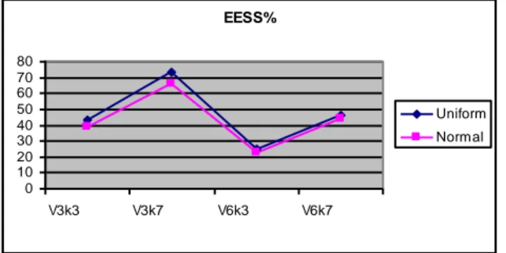
EESS% 0 10 20 30 40 50 60 70 80 V3k3 V3k7 V6k3 V6k7 Uniform Normal
Figure 1. The average values of the EESS% in CAs for different
number of input variables (V= 3 or V = 6), different number of clusters (k= 3 or k = 7), and for independent random variables with different distributions (uniform continuous or normal).
Point-biserial 0,2 0,25 0,3 0,35 0,4 0,45 0,5 V3k3 V3k7 V6k3 V6k7 Uniform Normal
Figure 2. The average values of the cluster point-biserial
correla-tion (PB) in CAs for different number of input variables (V= 3 or
V= 6), different number of clusters (k = 3 or k = 7), and for
in-dependent random variables with different distributions (uniform continuous or normal).
Influence of Number of Variables and Number
of Clusters on the Level of Some QCs
Simulations we have performed on data with independent random normal variates suggest that there is often a strong influence of the number of input variables (V ) and the num-ber of clusters (k) on most QCs (Vargha & Bergman,2015). In the following, this is detailed for four representative QCs (EESS%, PB, SC, and GDI24). Figures 1 to 4 show the av-erage values of the four QCs in CAs with different number of input variables (V= 3 or V = 6) and different number of clusters (k= 3 or k = 7) for independent random vari-ables of two different distributions (uniform continuous or normal). The simulated data for the CAs were the same that were used in the sections above (25 random samples for each combination of V and k).
It is seen in Figures 1-4 that the number of input vari-ables and the number of clusters had a high impact on the average values of the different QCs in two situations where no real cluster structure existed (independent variables in the value profile). Fixing the number of clusters, the aver-age value of a QC decreased with an increasing number of variables, and fixing the number of variables, the average value of a QC often increased with an increasing number of clusters. Exceptions are PB and GDI24 for V = 3. The average QC values belonging to CAs with uniformly dis-tributed independent random variables were never lower
GDI24 0,2 0,4 0,6 0,8 1 1,2 1,4 V3k3 V3k7 V6k3 V6k7 Uniform Normal
Figure 3. The average values of the GDI24 index in CAs for
differ-ent number of input variables (V= 3 or V = 6), different number of clusters (k= 3 or k = 7), and for independent random variables with different distributions (uniform continuous or normal).
Silhouette coefficient 0,2 0,3 0,4 0,5 0,6 0,7 V3k3 V3k7 V6k3 V6k7 Uniform Normal
Figure 4. The average values of the Silhouette coefficient (SC)
in CAs for different number of input variables (V = 3 or V = 6), different number of clusters (k= 3 or k = 7), and for independent random variables with different distributions (uniform continuous or normal).
than those obtained for normally distributed independent random variables, and for PB (see Figure 2) they were con-siderably larger. It is notable that for a CA (Ward type hier-archical, followed by a relocation) with 3 independent ran-dom variables, uniformly distributed, and with k= 7 clus-ters, it was found that the average EESS% was as high as 75%, whereas with 6 variables of the same type and k= 3 clusters the average level of EESS% was only around 25%. The findings we reported above show that in cases where no real cluster structure exists (independent variables), fairly high values of QCs can occur. Hence, there is a con-siderable risk that a researcher not aware of that falsely interprets that a real cluster structure has been found in a situation where there is no such structure. Hence it is im-portant to show that the cluster structure found could not have emerged from an analysis of a multivariate distribu-tion with independent variables. Therefore we propose that the QCs of the cluster structure obtained when analyzing a data set should be related to the QCs obtained by parallel control CAs of data sets characterized by independent vari-ables. A minimum requirement for having demonstrated a real cluster structure is that the control analyses show the QCs obtained when analyzing the real data set are higher than those obtained in the control analyses.
The MORI Index of Cluster Structure
and Significance Testing of a
Cluster-ing Solution
It is important to evaluate whether a QC indicates a “real” cluster structure and not just reflects a structure that could have emerged from analyzing random data. To help in this evaluation we propose an index, denoted MORI (acronym derived from Measure Of Relative Improvement), measur-ing the improvement of a QC obtained by analyzmeasur-ing real data as contrasted to the QC obtained by parallel analyses of random data with independent variables. MORI is com-puted according to Formula (6):
MORI= QC− QCr and QCbest− QCr and
. (6)
In Formula 6, QC is the quality measure of a cluster struc-ture that we would like to evaluate, QCr and is the average of QCs of CAs with simulated random data (performing at least 20 independent random replications), and QCbest is the (maximum) value of QC that is obtained when the cluster structure is perfect. Specifically, QCbest = 100 for EESS%, 1 for PB and SC, and 0 for HCmean. If QCbestis in-finite large, we suggest that the denominator of (6) is set to QCr and. In this case, MORI measures the improvement of QC relative to the base level of QCr and. It should be noted that similar validation approaches have successfully been applied in the context of exploratory factor analysis (see, e.g.,
http://pareonline.net/pdf/v12n2.pdf).
It is important to test the significance of a clustering so-lution by data simulation. This can be done by performing a one-sample t-test of whether the QC obtained when ana-lyzing the original data is significantly larger than QCr and, the average of QCs obtained with simulated random data. The number of independent iterations for this t-test is sug-gested to be at least 20-252. However, to have a reliable estimation of QC-levels and the MORI index, we suggest at least 100 iterations.
An additional important consideration is the choice of the type of control data sets that should be used. Possible options are:
1. Independent random permutations of the values of the input variables (seeVargha et al.,2015);
2. Independent random uniform variables; 3. Independent random normal variables.
In the case of option 1, the only difference between the original variables and the control set of variables is that the latter consists of independent variables; the marginal distri-butions are identical. In this case the MORI index indicates how much the relationship structure of the original vari-ables adds to forming appropriate clusters. In the case of the second option, the MORI index indicates how much the 2If a QC of a cluster structure is substantially better than the same type
of QC based on a series of random data set, 20-25 random replications suffice to show a clear significance by means of the t-test.
obtained cluster structure is better than a cluster structure created from a multivariate uniform distribution where no peaks occur. In the case of the third option, the MORI index indicates how much the obtained cluster structure is better than a cluster structure created from a multivariate normal distribution with only a single peak. For a good structure, a MORI index should be considerably larger than 0 for op-tions 2 and 3. For option 1, however, it is possible that a MORI index is small also for a “good” natural cluster struc-ture. In practice, this is rare but it can occur if in the original data set there are variables with a strongly bimodal distri-bution.
It should be noted that the K-Means module of ROPstat not only evaluates the “goodness” of a cluster structure by means of several QC measures (EESS%, HCmean, PB, etc.). The module also performs an internal validation analysis of the cluster structure by means of simulations of random data, performing the t-test mentioned above for each QC and computing the MORI index.
How should the size of an obtained MORI index be eval-uated? A rule of thumb could be used similar to the one used when evaluating the Cohen delta effect size measure, where 0.2 is regarded the minimal level that deserves to be interpreted, 0.5 can be regarded as the lower limit of a moderate effect size, and 0.8 the lower level of a high effect size (seeCohen,1977). For interpreting MORI we suggest for these three threshold levels of interpretation 0.15, 0.30 and 0.50, respectively. Certainly, this rule of thumb can be modified. For instance, in the case of a very high QCr and, the value of MORI can be more difficult to interpret.
An Illustrative Example
An illustration of QCs and MORI indices can be found in Table 1, based on data from the above mentioned minor-ity language shift study (Vargha & Borbély,2016). In the study, a K-means CA was performed with 5 standardized input variables (R/Wr: How often reads and writes in Ro-manian; Family: How often speaks Romanian with family members; Relig: How often speaks Romanian with church fellows; Ident: Level of Romanian identity; Attit: Level of positive attitude toward Romanian language) and a cluster-ing solution with 7 clusters was chosen. The solution had good properties according to criteria suggested byBergman et al.(2003), and it also conformed to theoretical expecta-tions.
Table 1 shows that the value levels of almost all QC mea-sures for the original data are rather high, suggesting a good cluster structure. The most important QCs (EESS% and HCmean) are highly significant (p < .001) for each type of simulation of random control variables. For these two QCs, the MORI indices are also substantial, ranging from 0.41 to 0.52. The significances and the MORI indices of PB and CLdelta are at a lower level, reaching an in-terpretable level only for the normally distributed random control variables. The SC MORI index indicates a moder-ately clear structure.
The only QC not showing a good clustering structure is GDI24 but, as explained before, this QC is of a type that is
Table 1. Values of six QCs and the MORI index in a K-means CA with 5 input variables and 7 clusters for 25 random replications, computed
by means of ROPstat.
QCs found when the original data were analyzed
Measure: EESS% HCmean PB CLdelta SC GDI24
Value: 75.97 0.498 0.439 1.225 0.671 0.407
Control: Findings found for random permutations of variable values
EESS% HCmean PB CLdelta SC GDI24
Mean: 59.03 0.848 0.43 1.208 0.576 0.535
t-value: 69.36 68.47 2.701 2.242 26.21 -9.147
p-value: <.001 <.001 0.012 0.034 <.001 <.001
MORI: 0.41 0.41 0.01 0.01 0.23 -0.24
Control: Findings found for uniformly distributed independent random variables
Measure: EESS% HCmean PB CLdelta SC GDI24
Mean: 52.49 0.983 0.392 1.116 0.508 0.704
t-value: 74.58 74.83 21.49 16.26 57.74 -19.56
p-value: <.001 <.001 <.001 <.001 <.001 <.001
MORI: 0.49 0.49 0.08 0.1 0.33 -0.42
Control: Findings found for normally distributed independent random variables
Measure: EESS% HCmean PB CLdelta SC GDI24
Mean: 49.55 1.044 0.314 0.889 0.485 0.561
t-value: 45.14 45.17 33.48 35.73 70.68 -8.353
p-value: <.001 <.001 <.001 <.001 <.001 <.001
MORI: 0.52 0.52 0.18 0.38 0.36 -0.28
Note.The t and p values refer to results from significance testing the original QC.
not optimal in person-oriented research. Nevertheless, its low level is an indication that there are some clusters that are very close to each other. This was verified by computing the pairwise cluster centroid distances using the Centroid module of ROPstat, and we found two clusters (CL1 and CL3) that are very close to one another with a distance of only 0.36 (with standardized variables), lower than the av-erage within-cluster distance (HCmean= 0.498). The only difference between the two cluster centroids is the attitude level toward Romanian language (average vs. very low). However, theoretical expectations support that these two clusters should be regarded as distinct clusters.
Discussion
A primary goal of the present paper was to draw the reader’s attention to the internal validity of clustering solu-tions and to the usefulness of appropriate QC measures for evaluating the “goodness” of a cluster structure. The paper presents several QCs that can be useful when carrying out classification analysis in a person-oriented context. Often the most useful QCs are those primarily measuring cluster homogeneity (EESS% and HCmean) but some QCs that in addition measure cluster separation can also be useful, for instance PB and SC.
Based on simulated data with independent variables, we showed that QCs can be strongly influenced by the number of clusters and the number of input variables (see Figures 1 to 4), and in cases where no real cluster structure
ex-ists (independent random variables), fairly high values of QCs can occur. This finding has also been pointed out by others (see Handl, Knowles, & Kell, 2005; Pardo, 2010). Hence, there is a considerable risk that a researcher not aware of that falsely interprets that a “real” cluster struc-ture has been found in a situation where there is no such structure.
To protect against such a false interpretation we pro-posed that the QCs of the cluster structure, obtained for a data set should be related to the QCs obtained by parallel control CAs of data sets characterized by independent ran-dom variables. A minimum expectation in a situation with a real cluster structure is that the QCs obtained when ana-lyzing the real data set are significantly higher than those obtained in appropriate control analyses. As an aid in eval-uating the extent of “real” cluster structure in the sense of the extent of structure beyond that what can be expected for data with no relationships between the variables we in-troduced the MORI index of relative improvement. It is helpful to compute MORI indices for three types of distri-butions with independent variables, namely random per-mutations of the variable values of the real data sample, independent random uniform variables, and independent random normal variables. Findings for each type of distri-bution display a different quality of the cluster structure in the validation process.
In general, the need for evaluation of cluster solutions has found considerable interest in the literature. Very close to the content of our paper are a number of articles by
Doug Steinley, and for the evaluation of cluster solutions the reader may wish to considerSteinley(2004,2006).
It should be pointed out that in the simulations and con-trol comparisons, QCs were almost solely based on
atypi-cal data; that is data without any real cluster structure
cre-ated by a random data generation process. This is a reason-able starting point, considering the extreme difficulty in ob-taining any kind of representative sample of data sets with real cluster structures, and considering that the informa-tion value and the interpretainforma-tion of the QCs are discussed in general and theoretical terms, using the findings obtained in the simulation experiments as illustrations of principles. Of course, in the broad family of classification analysis there exists other types of internal validation procedures than those we presented, for instance comparing cluster structure between random split-halves (Botta-Dukát,2008) or using bootstrapping (Bouwmeester et al.,2013).
It should be noted that the computation of the newly presented QCs (HCmean, CLdelta) and the whole valida-tion process can easily be performed by means of the K-means (Relocation) module of the ROPstat statistical soft-ware (see
www.ropstat.com
orVargha et al.,2015). An application of the ROPstat module was presented in the pre-vious section. However, it would also be useful to present a complete template study of CA in a person-oriented con-text with the purpose to provide a guide for the researcher to navigate the confusing jungle of person-oriented cluster analysis-based approaches. This task is planned to be the focus of a future article.Acknowledgements
We thank the numerous valuable comments and sugges-tions of the editors, Wolfgang Wiedermann and Alexander von Eye, on an earlier draft of our paper. The preparation of the present article was supported by the National Research, Development and Innovation Office of Hungary (Grant No. K 116965).
References
Bergman, L. R. (1988). You can’t classify all of the people all of the time. Multivariate Behavioral Research, 23, 425–441. Bergman, L. R., & Magnusson, D. (1997). A person-oriented
ap-proach in research on developmental psychopathology.
De-velopment and Psychopathology, 9, 291–319.
Bergman, L. R., Magnusson, D., & El-Khouri, B. M. (2003).
Study-ing individual development in an interindividual context. a person-oriented approach. Mahwa, New Jersey, London: Lawrence-Erlbaum Associates.
Botta-Dukát, Z. (2008). Validation of hierarchical classifications by splitting dataset. Acta Botanica Hungarica, 50(1–2), 73– 80.
Bouwmeester, W., Moons, K. G. M., Kappen, T. H., van Klei, W. A., Twisk, J. W. R., Eijkemans, M. J. C., & Vergouwe, Y. (2013). Internal validation of risk models in clustered data: A com-parison of bootstrap schemes. American Journal of
Epidemi-ology, 177(11), 1209–1217.
Cohen, J. (1977). Statistical power analysis for the behavioral
sciences(rev. ed. ed.). New York: Academic Press.
Cohen, J. (1992). A power primer. Psychological Bulletin, 112(1), 155–159.
Desgraupes, B. (2013). Clustering Indices. University Paris Ouest,
Lab Modal’X, April 2013. https://cran.r-project .org/web/packages/clusterCrit/vignettes/ clusterCrit.pdf.(Downloaded: August 28, 2015) Desgraupes, B. (2015). ClusterCrit: Clustering Indices,
Compute clustering validation indices. 2015-08-31. http://stat.ethz.ch/CRAN/web/packages/ clusterCrit/index.html. (Downloaded: September 26, 2015)
Glass, G. V., & Hopkins, K. D. (1996). Statistical methods in
edu-cation and psychology(3rd ed.). Boston: Allyn & Bacon. Handl, J., Knowles, J., & Kell, D. B. (2005). Computational cluster
validation in post-genomic data analysis. Bioinformatics,
21(15), 3201–3212.
Jegatha Deborah, L., Baskaran, R., & Kannan, A. (2010). A survey on internal validity measure for cluster validation.
Inter-national Journal of Computer Science & Engineering Survey (IJCSES), 1(2). (http://www.airccse.org/journal/ ijcses/papers/1110ijcses07.pdf)
Kaufman, L., & Rousseeuw, P. J. (1990). Finding groups in data:
an introduction to cluster analysis. New York: John Wiley & Sons.
Marszalek, J. M., Barber, C., Kohlhart, J., & Holmes, C. B. (2011). Sample size in psychological research over the past 30 years. Perceptual and Motor Skills, 112(2), 331–348. Pardo, M. (2010). Clustering.http://lectures.molgen.mpg
.de/algsysbio10/clustering.pdf. (Downloaded: April 26, 2015)
Rendón, E., Abundez, I., Arizmendi, A., & Quiroz, E. M. (2011). Internal versus external cluster validation indexes.
Inter-national Journal of Computers and Communications, 5(1), 27–34.
Steinley, D. (2004). Properties of the Hubert-Arable Adjusted Rand Index. Psychological Methods, 9(3), 386–396. Steinley, D. (2006). K-means clustering: a half-century synthesis.
British Journal of Mathematical and Statistical Psychology,
59(1), 1–34.
Vargha, A., & Bergman, L. R. (2015). Finding typical pat-terns in person-oriented research within a cluster-analytic framework using ROPstat. Conference on Person-Orienteed Research. May 8 and 9, 2015, Vienna, Austria.
Vargha, A., & Borbély, A. (2016). Modern mintázatfeltáró módsz-erek alkalmazása a kétnyelv˝uség kutatásában[the applica-tion of modern pattern-oriented methods in the research of bilingualism]. In V. M. Kissné, Z. Puskás-Vajda, J. Rácz, & V. Tóth (Eds.), A pszichológiai tanácsadás perspektívái.
tisztelg˝o kötet ritoók magda 80. születésnapjára(pp. 173– 186). Budapest: L’Harmattan.
Vargha, A., Torma, B., & Bergman, L. R. (2015). ROPstat: a general statistical package useful for conducting person-oriented analyses. Journal for Person-Oriented Research,