Stomach data from pelagic research survey bring new information in cod feeding pattern in the South-Western Baltic sea

(1)

Department of Aquatic Resources

Stomach data from pelagic research survey

bring new information in cod feeding pattern

in the South-Western Baltic sea

(2)

Stomach data from pelagic research survey bring new

information in cod feeding pattern in the South-Western Baltic

sea

Federico Maioli

Supervisor:

Assistant supervisor:

Examiner:

Michele Casini, Swedish University of Agricultural Sciences, Department of Aquatic Resources

Håkan Wennhage, Swedish University of Agricultural Sciences, Department of Aquatic Resources

Sara Königson, Swedish University of Agricultural Sciences, Department of Aquatic Resources Credits: Level: Course title: Course code: 30 hec

Second cycle, A2E

Indipendent project in biology EX0895

Place of publication: Lysekil Year of publication: 2019

Online publication: https://stud.epsilon.slu.se

(3)

Pelagic and demersal cod (Gadus Morhua) specimens were collected respectively during a pelagic and a demersal survey in the Eastern Baltic sea in the fourth quarter of the years 2015-2017. Stomach contents were analysed and compared for the pur-pose of evaluating differences in the diet among pelagic and demersal specimens. Furthermore, generalized additive models (GAMs) were employed to investigate the daily fluctuations of stomach content weights of this predator. My results showed significant differences in the diet composition of demersal and pelagic cod mainly attributable to the higher weight share of sprat in the pelagic stomachs. Moreover, a remarkable diel variation in the stomach contents weights was present, indicating morning and evening peaks. The present study furnished novel insights into cod feed-ing pattern in the South-Western Baltic Sea. The implications of these findfeed-ings for stock assessment multispecies models are also briefly discussed.

Keywords: Eastern Baltic Cod, diet, stomach data.

(4)

Quantifying trophic interactions (who is eaten by whom, and how much, in a given ecosystem) is essential to fully understand how a natural system works. The analysis and the identification of stomach contents is often the preferred mean of accessing this information. Trophic interactions are further recog-nized as a key aspect in the management of fishery resources and several modelling approaches that account for these interactions have been developed and collectively called multispecies models.

In the Baltic Sea region, most of the multispecies models have focused on the interactions between the predator cod and its preeminent prey, the clupeids sprat and herring. These species are of great economic and ecological value for the Baltic Sea, and historical abundance and stomach data are easily ac-cessible. However, stomachs of cod are sampled, for monitoring purposes, exclusively with bottom trawls while the regular presence of this predator in the open water suggests that its diet may differ from what exclusively dis-cerned from the bottom trawls. In my thesis, I specifically asked whether cod captured in the water column has a different diet of the cod captured near the sea bottom. Furthermore, I investigated the around-the-clock variation in cod stomach content weights. The results of my analysis showed significantly dif-ferences in the diet between cod captured near the bottom and in the water column mainly attributable to the fact that cod eats far more sprat while in the water column. Moreover, diel variation in stomach contents weights sug-gested that cod eats more during morning and evening. Thus, sampling for diet analyses is recommended also in the pelagic and covering the whole day (around-the-clock). The implications of these findings in multispecies models are also briefly discussed.

(5)

Governed by unique climatic and hydrographical conditions, the Baltic Sea is a semi-enclosed postglacial basin with a strong salinity gradient from the entrance to the inward part (Snoeijs-Leijonmalm, Schubert, & Radziejewska, 2017). The young geological age of this water body (only 8000 years old) conjointly with its prevailing brackish conditions led to low species diversity and relatively simple structure of the food web (Jan Horbowy, 2005; Sandström et al., 2018). Ecosystem processes in the Baltic sea have been studied for decades and the literature has been increasing almost exponentially over the last 50 years establishing a relatively comprehensive perception of the ecosystem functioning. This region is especially recognized as a spearhead with respect to multi-species studies (Casini et al., 2008; Casini et al., 2009). Investigating trophic interactions is central to a multi-species framework and the assessment of trophic interactions, in terms of feeding habits, is further recogni-zed as a key aspect in fisheries management (Chipps & Garvey, 2007). Omitting such information may lead to gross miscalculations in stock assessment estimations (Horbowy, 1996) - that is, estimations of the status of a managed fish unit.

As a matter of fact, several multi-species modelling approaches that take trophic interactions into account were developed in the Baltic Sea, e.g. the multi-species virtual population model (Helgason & Gislason, 1979), the Stochastic Multi Species (SMS) model (Lewy & Vinther, 2004), Gadget (Begley, 2012) and Ecopath with Ecosim (Christensen, Walters, & Pauly, 2005). Moreover, efforts have been made to employ these models in fisheries management.

The Atlantic cod (Gadus Morhua) is the dominant fish predator in the offshore Bal-tic sea and plays a crucial role in the ecosystem dynamics of this region (Casini et al., 2008). Owing to the great economic and ecological value of this gadoid and its preeminent prey, the clupeids sprat and herring, in conjunction with the existence of extensive historical abundance and stomach data, the vast majority of multi-species models have focused on the interaction between these three multi-species. In the Baltic region, cod is assessed and handled as two separate stocks: western and

(7)

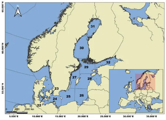
eastern Baltic cod, the former located in ICES Subdivisions (SDs) 22-24, the latter, subject of this study, in SDs 24-32 (Fig. 1).

Figure 1. Baltic Sea with the ICES Subdivisions (SD).

In the Baltic sea, cod hatch as a pelagic planktivore and feed mainly on copepods and cladocerans up to the size of 4-5 cm when benthic preys are introduced in the diet (Hüssy, John, & Böttcher, 1997) and settle in the demersal zone. Fish consump-tion, particularly on the clupeids sprat and herring, increases in conjunction with the size of the predator, even though benthic invertebrates are still present in the diet (Huwer et al., 2014).

For field studies, as well as for monitoring purposes, stomach contents data are often the only available mean providing quantitative information on trophic interactions (Amundsen, Gabler, & Staldvik, 1996; Chipps & Garvey, 2007 ). In the Baltic sea, The Baltic International Trawl Survey (BITS; ICES, 2017a), coordinated by the In-ternational Council for the Exploration of the Sea (ICES) is ordinarily employed for monitoring cod density and, inter alia, for sampling stomachs of cod in the demersal habitat. This demersal survey is therefore the main source providing input data for the multi-species models. Additionally, trophic studies on cod has been focused on its diet in the demersal habitat while a comprehensive description of cod feeding habits in the pelagic zone still lacks in the Baltic Sea (but see Hüssy et al., 1997 for cod juvenile stage). However, despite being a demersal species, the pelagic presence

(8)

of this predator is well documented and often reflects Diel Vertical Migration (DVM) at a population level (Hüssy et al., 1997 ; Strand & Huse, 2007; Casini et al., 2019). Besides that, seek for food, seasonal spawning and avoidance of unfa-vourable conditions in deeper strata are other reasons of occurrence of cod in the pelagic habitat (Engås & Godø, 1986; Godø & Wespestad, 1993). More recently, in the Baltic Sea, the increasing extent of hypoxic and anoxic areas in deeper strata has been related to the cod relocation in the pelagic habitat, acting as a refuge from these prohibitive conditions.

As a result, this predator regular occurrence in pelagic waters suggests that its diet may differ from what exclusively discerned from a demersal survey like BITS. An opportunity to analyse the diet composition of this species in the pelagic habitat is provided by another ICES-coordinated survey, the Baltic International Acoustic Survey (BIAS), mainly employed for monitoring small pelagic fishes like herring and sprat. The sampling design of this survey would further allow to study cod diet in the pelagic habitat around-the-clock. The aim of this study was to: i) describe and compare the diet of cod captured in the demersal habitat and in the pelagic habitat; ii) disclose patterns of food consumption in relation to the time of the day; iii) dis-cuss the potential implications for multispecies assessment models.

(9)

2.1 Stomach data

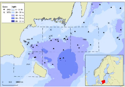
Stomach samples of Baltic cod were collected during the BITS and the BIAS sur-veys in the fourth quarter (Q4) of 2015, 2016 and 2017 by the Institute of Marine Research, Lysekil. The stomach samples covered ICES subdivisions (SD) 25, 26 and 27 (Fig. 2) but only data from SD 25 complied with the requirements of an adequate number of stomachs and were employed in the analysis.

Figure 2. Sampling stations of the BIAS and BITS surveys in SD 25.

(10)

According to the BITS protocol the sampling stations are depth-stratified and se-lected randomly within each SD from a set of known trawlable sites. Conversely, BIAS hauls are rather, but not necessarily, performed in correspondence of large shoal of fishes as detected by echosounder. Stomachs were sampled according to a length stratified design: one stomach for every 1cm length class per haul. The depth of the BITS trawl hauls ranged between 35 and 67 m. For the BIAS survey, the depth of the trawl hauls varied between 15 and 56 m, while the distance from the sea bottom to the headrope of the net ranged from 19 to 72 m. I estimated that no more of 10% of the BIAS and BITS hauls vertically overlapped considering their vertical opening and trawl depth. The demersal trawl hauls were performed between 06:45 and 13:30 UTC (shooting time of the hauls) while the midwater trawl hauls were carried out around-the-clock. The standard duration of the hauls were of 30 minutes for both the surveys. After the capture, fishes were sorted into species and cod total length, total weight, and gutted weight were annotated as well as the metadata for the hauls (e.g. latitude and longitude, trawling time, bottom depth). Signs of regurgitation were identified onboard by remains of prey in the mouth and everted swim bladder, but also due to stage of the gallbladder (see ICES, 2017). For the latter case, when the fish was associated with a gallbladder stage indicating a feeding state and had an empty stomach, the fish was marked as regurgitated. All stomachs that were everted or showed evidence of regurgitation were not collected. The other stomachs were extracted on board and immediately frozen. In total 943 stomachs were sampled in the SD 25, 635 from the BITS, 308 from the BIAS sur-vey. The taxonomic identification of the stomach contents was performed by the Sea Fisheries Institute of Gdynia, Poland. Each stomach was categorized according to its fullness (1 = full, 0 = empty). The food items were identified to the lowest taxonomic level possible. The number of each prey in the stomach was counted and the weight of the prey category was annotated. Whenever possible, prey items were weighted individually. Each prey item was also categorized into three digestion stages: 0 = undigested or only minimal signs of digestion; 1 = partly digested and 2 = greatly digested, only hard parts like scales or shells left. Prey with digestion stage of 0 (undigested) were disregarded for the subsequent analysis owing to the fact they were likely to be eaten inside the haul (Hopkins & Baird, 1975). Prey items without annotated weight have been disregarded as well.

(11)

2.2 Data analysis

2.2.1 Describing differences in diet composition

Diel vertical migrations of cod in the water column suggest that its diet may vary in composition according to a daily cycle. As a matter of fact, prior to the analysis, a visual inspection of the stomach contents data indicated possible differences in the diet between the pelagic trawl hauls (i.e. BIAS) performed night-time (17:30–05:30 UTC) from the ones performed daytime (05:30–17:30 UTC). Hence, these two sam-pling groups were kept separated. Eventually, 3 groups were analysed and com-pared: one demersal caught with trawl survey (BITS) and two pelagic caught with pelagic hauls (BIAS), one of which caught during daytime, the other caught during night-time. With the purpose of minimizing the spatial variability among the sam-pling groups exclusively ICES squares covered by BITS, day-time BIAS and night-time BIAS hauls were considered in this analysis i.e. 39G4, 40G4, 40G5, 40G6 (Fig. 3).

Figure 3. Sampling station of the BIAS and BITS surveys in SD 25 selected for the diet composition analysis. Dashed lines indicates ICES rectangles.

(12)

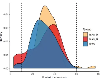
Finally, only adult cod with size ≥ 30 cm (when cod start to consistently introduce fishes in its diet; Huwer et al., 2014) were considered. Specimen > 60 cm were disregarded because underrepresented (Fig. 4).

The dietary importance of each prey item was estimated by percent composition by weight (%Wi) and frequency of occurrence (% F), calculated as follow:

% Wi = (total weight of prey i total weight of prey i)⁄ *100

% Fi = (number of stomachs with prey i total number of stomachs)⁄ *100 Prey composition by weight has been chosen over other indices because it reflects somehow the energetic importance of different prey types and provides a better comparability between different food items (Chipps & Garvey, 2007), it is as well a typical input for multispecies models.

Feeding strategy and prey importance were assessed for each sampling group using the graphical method of Costello (1990). Within this approach, abundance is plotted against the frequency of occurrence in order to visually acquire information about relevant components of the trophic niche of the predator.

2.2.2 Statistical multivariate analysis

Differences in diet composition were evaluated by a permutational multivariate analysis of variance (PERMANOVA; Anderson, 2005)calculated on Bray-Curtis dissimilarity matrix (Clarke & Warwick, 1994). Prior to that, data were fourth root transformed and the homogeneity of multivariate dispersion was checked by PERMDISP (Anderson, Ellingsen, & McArdle, 2006). Similarity percentages (SIMPER; Clarke & Warwick, 1994) with a permutation test was used to identify which dietary categories were an important component of their contribution to dis-similarities among groups. In order to reduce the number of variables involved in the multivariate analysis, abundant prey species in the stomachs and species that are mentioned in literature as important prey for cod were kept separated, the other prey were pooled into wider taxonomic categories (Table 7, Appendix). Individual stom-achs were treated as a random sampling unit and prey item weights were standard-ized to the total weight of the stomach to account for differences in the gut fullness.

(13)

2.2.3 Modelling diel variation of stomach contents

Temporal variation of stomach contents weight were investigated using generalized additive models (GAMs; Hastie & Tibshirani, 1987). The chosen approach is some-way similar to the delta–gamma (∆–Γ) along the guidelines of Stefánsson (1996) and consisted of two separate elements: a model for the probability of an empty/full stomach and a model for the content weights of a full stomach. Within this approach the act of feeding is considered separately from the amount of food consumed. Both these components are ecologically meaningful since the proportion of empty/full stomachs may be seen as an indicator of either feeding or nonfeeding behaviour, while the quantity of food observed in full stomachs as a measure of the amount eaten (Stefánsson & Pálsson, 1997). The emptiness–fullness of a stomach (0 or 1) was modelled fitting a binomial error distribution with a logit link function. On the other hand, the total amount of food consumed, was modelled using a Gamma error distribution with a logit link function (Steffanson, 1996; Waiwood, Smith, & Petersen, 2008). The total amount of food in the latter model was fourth root trans-formed to stabilize the variance. The models were respectively formulated as fol-low:

empty/full = 𝛽 + Cruise + Year + s(Predator size) + s(Time) + s(Time, Cruise) + s(Time, Predator size) + s(Long, Lat) + s(Bottom depth) + 𝜀

√amount of food eaten

4

= 𝛽 + Cruise + Year + s(Predator size) + s(Time) + s(Time, Cruise) + s(Time, Predator size) + s(Long, Lat) + s(Bottom depth) + 𝜀

where 𝛽 is the intercept, s is an isotropic smoothing function (thin-plate regression spline; Wood, 2003), Cruise represent the two survey (BITS and BIAS). Predator size is the total length of the cod and was included in the model to account for size-related differences in the food consumption. Time is the haul shooting time. A cyclic cubic regression spline was employed to smooth this term in order to conform it to a cyclic pattern. The interaction of the Time term with Cruise was included because of the potential differences in diel pattern of stomach contents depending on the cruise. Time is further present as interactive term with Predator size because stom-achs of different lengths of cod may follow different daily pattern. Long and Lat represent cod spatial distribution, accounting for the fact that stomach contents may be not spatially homogeneous. Bottom depth was included because it may influence prey availability, mainly zoobenthos. Finally, 𝜀 is the error term. Final model selec-tion have been carried out dropping individual explanatory variables via a backward stepwise selection approach based on statistical significance (Wood, 2008). Preda-tors with size ≤ 10 cm and ≥ 60 cm were not considered in the analysis because

(14)

underrepresented (Fig. 4). Due to the high flexibility of GAMs towards unbalanced design in terms of Latitude and Longitude (Casini et al. 2019), the full dataset was employed.

Figure 4. Predator size distributions. Dashed lines indicate the outer limit of the size of the specimen selected for the analysis. BIAS_D, daytime BIAS; BIAS_N, night-time BIAS.

(15)

3.1 Diet composition

3.1.1 Digestion stage

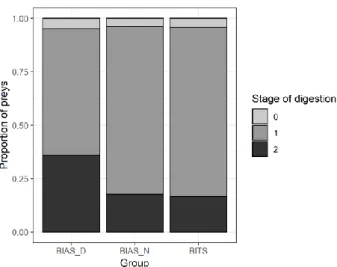
Stage of digestion coded as 1, indicating partial digestion of the prey, was the most common digestion stage (Fig. 5). Digestion stage 2, greatly digested, appeared more frequently in the samples from daytime BIAS.

Figure 5. Proportion of prey digestion stage for specimen ≥ 30 and ≤ 60 cm. 0, undigested or only

minimal signs of digestion; 1, partly digested; 2, greatly digested, only hard parts like scales or shells left.

(16)

3.1.2 Diet and feeding strategy description

Stomach content analysis led to the identification of 31 food items belonging to five main taxa: Teleostei, Crustacea, Polychaetae, Mollusca and Priapulida (Table 1). Cod diet consisted mainly of clupeids, ranging from approximately 80% of the weight abundance up to 93% depending on the sampling group. The weight propor-tion of sprat in the diet was 12-fold higher than that of herring in individuals caught during daytime BIAS and 3-fold higher for specimen captured during night-time BIAS. On the other hand, demersal captured individuals showed an almost even partition between the two clupeids (both %W and %F). The three-spined stickleback

Gasterosteus aculeatus was occasionally recorded in the pelagic samples while

ac-counted for about 4% of the weight share and 10% of the frequency in the demersal ones. Cannibalism has been observed only in stomach samples from the BITS sur-vey. Gobiidae were encountered sporadically both in the demersal and pelagic sam-ples. The most important crustaceans in terms of weight and frequency were Saduria

entomon, Diastylis rathkei and Mysis mixta. The Polychaeta Bylgides Sarsi was an

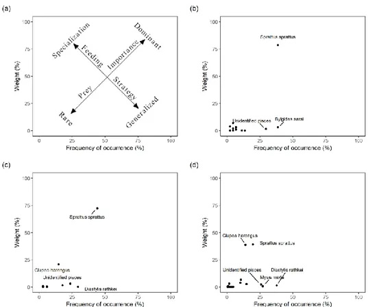
import prey item exclusively in stomachs from Day-time BIAS (%W = 3, %F = 38.64). Mollusca and Priapulida have been seldom recorded. The Costello plot iden-tified sprat as the dominant prey and revealed a high degree of specialization of cod towards this prey regardless of the sampling group (Fig. 6). Nevertheless, the degree of specialization towards sprat decreased in stomach samples from BITS. Herring, on the other hand, was of considerable importance in BITS and night-time BIAS stomachs while appeared as a rare prey in day-time BIAS samples. In this study all prey categories except clupeids showed a low abundance (<10 % of weight share) and a low frequency of occurrence, suggesting that cod in this region often enriches his diet consuming a wide variety of prey whenever available. This situation is em-phasized for BITS samples, even though supported from a larger sample size.

Table 1. Diet composition for specimen ≥30 and ≤ 60 cm. %W, percentage in weight; %F, frequency of occurrence. BITS Daytime BIAS Night-time BIAS W (%) F (%) W (%) F (%) W (%) F (%) Teleostei Sprattus sprattus 39.16 19.74 78.49 38.64 72.37 44.12 Clupea harengus 38.64 14.04 6.91 4.55 20.79 14.71 Gadus morhua 0.72 0.88 unidentified Clupeidae 6.73 10.53 3.08 6.82 0.52 2.94

(17)

BITS Daytime BIAS Night-time BIAS Gasterosteus aculeatus 3.82 10.09 1.87 4.55 0.75 2.94 Enchelyopus cimbrius 3.09 1.75 unidentified Pisces 2.21 25.88 1.54 29.55 3.11 23.53 Zoarces viviparus 0.37 0.44 unidentified Gobiidae 0.08 2.19 0.12 2.27 0.16 5.88 Crustacea Saduria entomon 2.75 14.91 0.93 6.82 1.57 17.65 Diastylis rathkei 1.46 37.72 0.03 13.64 0.08 29.41 Mysis mixta 0.7 27.19 0.07 11.36 0.01 5.88 Crangon crangon 0.08 3.51 0.06 4.55 0.16 2.94 Gammarus sp. 0.03 4.82 0.03 5.88 Neomysis integer 0.01 3.51 0.02 2.27 0.01 5.88 Pontoporeia femorata 0.01 2.19 <0.01 2.27 0.02 5.88 Monoporeia affinis <0.01 0.88 Idotea sp. <0.01 0.44 Amphipoda <0.01 0.44 Palaemon elegans 0.09 2.27 Hyperia galba <0.01 2.27 <0.01 2.94 Polychaetae Bylgides sarsi 0.07 3.07 3 38.64 0.42 5.88 Halicryptus spinulosus 0.04 3.51 <0.01 2.27 unidentified Polychaeta <0.01 0.88 Nephtys ciliata 3.77 2.27 Mollusca unidentified Bivalvia 0.01 0.44 Mytilus sp. <0.01 1.32 0.01 2.27 Limecola balthica 0.01 2.63 Priapulida Priapulus caudatus 0.01 0.88 unidentified Priapulida <0.01 0.88

(18)

Figure 6. Costello plot for specimen ≥ 30 and ≤ 60 cm (a) Interpretation of the plot: the two diagonal

axes represent the importance of prey (dominant vs. rare) and the predator feeding strategy (specialist vs. generalist). (b) Daytime BIAS. (c) Night-time BIAS. (d) BITS. Only prey item with frequency of occurrence or abundance ≥ 20 % were shown.

(19)

3.2 Multivariate analysis

Pooled food categories for the multivariate analysis were aggregated as showed in Fig. 7. The PERMANOVA analysis showed significant differences in dietary com-position among groups (p = 0.001; Table 2). Posterior pairwise PERMANOVA comparisons with Bonferroni correction revealed significant differences between day-time BIAS and BITS (p = 0.003), day-time BIAS and night-time BIAS (p = 0.024), night-time BIAS and BITS (p = 0.033) (Table 3).The PERMDISP analysis yielded no significant differences (p = 0.313; Table 4), suggesting that the differ-ences obtained with PERMANOVA were not due to multivariate dispersion. SIM-PER analysis, with a permutation test (Table 5), identified the species for which the differences among groups were an important component of their contribution to dis-similarities: BITS vs. daytime BIAS, Sprattus sprattus (22.8%; p = 0.012) and

Bylgides sarsi (18.8%; p = 0.001); BITS vs. night-time BIAS, Sprattus sprattus

(24.7%; p = 0.008); daytime BIAS vs. night-time BIAS, Sprattus sprattus (28.5%; p = 0.001) and Bylgides sarsi (21.1%; p = 0.001). Sprat resulted the main contributor to the dissimilarities between the sampling groups showing, on average, higher val-ues in night-time BIAS samples, followed by daytime BIAS. Bylgides sarsi repre-sented another considerable source of variation among groups, peaking in daytime BIAS.

(20)

Table 2. Permutational analysis of variance (PERMANOVA) based on Bray-Curtis distances. Df, de-grees of freedom; SS, sum of squares; MS, mean squares; Pseudo-F, Pseudo-F statistics; R2_,

coeffi-cient of determination; P (perm), permutational p-value.

Df SS MS Pseudo-F R2 _{P (perm)}

Group 2 5.035 2.51737 6.9821 0.044 0.001

Residuals 303 109.246 0.36055 0.956

Total 305 114.280 100.000

Table 3. Pairwise permutational analysis of variance (PERMANOVA) based on Bray-Curtis distances. Pseudo-F, Pseudo-F statistics; P (perm), permutational p-value; adj. P, adjusted p-value after Bon-ferroni correction.

Comparison Pseudo-F P (perm) adj. P

BITS vs. daytime BIAS 11.401 0.001 0.003

BITS vs. night-time BIAS 3.2016 0.011 0.033

daytime BIAS vs. night-time BIAS 4.3109 0.008 0.024

Table 4. PERMDISP, multivariate homogeneity of groups dispersions. DF, degrees of freedom; SS, sum of squares; MS, mean squares. F Model, F model statistics; P (perm), permutational p-value.

Df SS MS F Model P (perm)

Group 2 0.0661 0.033026 2.9322 0.057

Residuals 303 3.4128 0.011263

Table 5. SIMPER analysis. Avg, average; Cumsum, cumulative sum; P (perm), permutational p-value.

Comparison Prey Avg i term Avg ii

term

Cumsum (%)

P

(perm) BITS vs. daytime BIAS Sprattus sprattus 0.160 0.360 22.8 0.012

Bylgides sarsi 0.015 0.326 41.6 0.001

Unidentified Pisces

0.210 0.192 59.6 0.393 BITS vs. night-time BIAS Sprattus sprattus 0.160 0.386 24.7 0.008 Cumacea 0.186 0.230 44.1 0.051 Unidentified

Pisces

0.210 0.101 59.9 0.937 daytime BIAS vs. night-time

BIAS Sprattus sprattus 0.360 0.386 28.5 0.001 Bylgides sarsi 0.326 0.050 49.6 0.001 Unidentified Pisces 0.192 0.101 65.1 0.919

(21)

3.3 Statistical modelling of the stomach contents

3.3.1 Binomial model

The final binomial model selected incorporated the term Cruise, Predator size and the spatial component, Longitude and Latitude explaining together only 12.8% of the total variance (Table 6). Inspection of the residuals did not reveal significant departures from the model assumptions. The fitted effect of the cruise indicated that individuals captured during BITS had higher chance of owning a non-empty stom-ach compared to the specimens captured during BIAS (Fig. 8a, Fig. 9). Moreover, as the predator size increased, the probability of encountering a non-empty stomach diminished (Figure 8b), however this pattern was not clear after the size of 45 cm. Lastly, the partial effect of the spatial location (Fig. 8c) indicated that the probabil-ities of hitting an empty or a non-empty stomachs are not spatially homogeneous and higher probabilities of hitting a non-empty stomachs are met in the proximity of SD 26.

Table 6. Summary statistics of the GAMs employed. Only variable retained in the final model are shown. Dev %, explained deviance; df, degrees of freedom; P, p-value.

Model Variables retained Dev % df P

Binomial Cruise 12.6 1 <0.001 Predator size 3.83 <0.001 Long:Lat 10.71 0.015 Gamma Cruise 35.7 1 <0.001 Predator size 5 <0.001 Time (UTC) 2.52 0.001 Bottom depth 2.55 <0.001

(22)

Figure 8. Model results of the binomial GAM. (a) Partial effect of cruise. (b) Partial effect of predator size. (c) Partial effect of the spatial location. Confidence bands in grey. Isolines represent sites with equal predicted probability of hitting a full stomach.

(23)

3.3.2 Gamma model

The final gamma model selected incorporated the terms cruise, predator size, time of the day (UTC) and bottom depth, explaining together 35.7% of the total deviance (Table 6). Inspection of the residuals did not reveal significant departures from the model assumptions (see Figure 1 Annex). The parametric coefficients indicated that total weight of the stomach contents was higher in the BIAS samples and lower in the BITS ones (Fig. 9a; Fig. 10). Additionally, total weight of stomach contents increased progressively with predator size as showed in Fig. 9b. A diel pattern was appreciable for the pelagic specimen, showing morning (around 10:00 UTC) and evening peaks (around 20:00 UTC; Fig. 9c). Some differences are observed as well regarding the bottom depth effect (Fig. 9d), particularly shallow waters appear to be associated with higher total weight of stomach contents.

Figure 10. Model results of the binomial GAM. (a) Partial effect of cruise. (b) Partial effect of predator size. (c) Partial effect of time of the day. (d) Partial effect of the bottom depth (m). Confidence bands in grey.

(24)

(25)

This study explored the diet composition of cod with respect to the occupied habitat, i.e. demersal vs. pelagic and time of the day. My results from the demersal BITS survey seem to generally agree with the most recent literature considering the weight share of the prey (Neuenfeldt & Beyer, 2003; Pachur & Horbowy, 2013). However, differences are present for specific prey items, Pachur & Horbowy (2013), for ex-ample, observed near the half weight share of herring compared to my results. Nev-ertheless, their study incorporated the first and the fourth quarter and was conducted within the Polish Exclusive Economic Zone, suggesting that dissimilarities in the diet composition may exist due to seasonality and location. On the other hand, to my knowledge, my study represent the only available description of cod diet in the pelagic habitat for the Baltic sea.

Diet composition of cod appeared to change significantly in relation to the occupied habitat. Especially, the weight proportion of sprat seemed to account for most of the dissimilarities among cruises showing, on average, higher weight share in the sam-ples from the pelagic survey. A peculiar outcome of the analysis considering day-time BIAS stomach samples was the relative high presence of the Polychaetae

Bylgides sarsi. Despite being considered a demersal dweller, this worm is found to

have semi-pelagic habits. The vertical migrations of this polychaetes may be related to the environment occupied. Indeed, B. sarsi often lives on ooze bottoms that tends to be oxygen deficit and may perform vertical movements towards more oxygenated layers (Sarvala, 1971). Howsoever the considerable presence of this annelid in the stomach contents of pelagic individuals may be restricted to a fortuitous event, since a discrete number of stomachs containing this species came from a few hauls. Be-yond that, herring during daytime was an important prey in samples from the de-mersal samples and appeared only rarely in pelagic stomach samples. Additionally, the Costello plots indicated that while demersal captured individuals showed a sim-ilar degree of specialization towards sprat and herring, pelagic specimen are highly specialized towards sprat only. Cannibalism was only observed in demersal

(26)

samples, however the low frequency of occurrence of this phenomenon (<1%) may reflect a larger sample size compared to the pelagic survey.

The higher weight share of sprat in the diet from pelagic samples and of herring in the demersal samples during daytime is consistent with cod-clupeids vertical over-lap in the water column of the Baltic Sea, that sees sprat occurring in intermediate water layers, near the halocline and in bottom waters, while herring and cod occur-ring exclusively close to the halocline and in the bottom water (Neuenfeldt & Beyer, 2003).

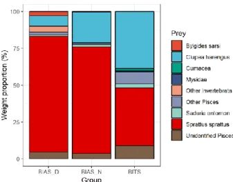
Significant difference in the diet were also detected within the pelagic cruise sepa-rating daytime from night-time samples mainly due to the higher frequency of oc-currence of sprat in the stomachs during the night. Additionally, herring was an im-portant prey only in night samples from the pelagic survey. Both clupeids are known to perform diel vertical migrations (DVM), descending at dawn, aggregating during daylight hours and ascending at dusk (Orłowski, 2000; Orlowski, 2001; Casini et al. 2004). Tracking diet composition changes of BIAS samples throughout the day (Fig. 12) seemed to be coherent with the DVM described. Indeed, the weight share of herring in cod stomachs increases in the pelagic samples as the night approaches, most likely because it becomes available in the pelagic zone. Also cod is able to perform DVMs. During night-time Strand & Huse (2007) simulations with an adap-tive individual-based model indicated that cod would stay in the pelagic zone to attain neutral buoyancy and save energy. This pattern seems to conform with the higher catch per unit effort (CPUE) in the pelagic water during night-time reported by acoustic surveys and, as argued by fishermen, the lower catchability of the com-mercial vessels fishing with bottom trawls during the night (Casini et al., 2019). Additionally, Brunel (1966) reported that Northwest Atlantic cod change their ver-tical migration strategy over time, highlighting two extreme cases: a demersal strat-egy in which cod ascend to midwater during night and descend to the bottom during the day and a pelagic strategy in which the cod stay in midwater for a prolonged period. However, the presence of fresh benthic food items in the stomachs of Baltic cod captured with pelagic hauls in my study indicates that individual fish may switch between the demersal and the pelagic habitat and are not vertically stationary outside the main DVM patterns (Neuenfeldt & Beyer, 2003).

(27)

Figure 12. Diet composition of BIAS captured specimens throughout the day.

My study also indicated diel fluctuations of stomach content total weights showing morning and evening peaks. This result is consistent with similar studies conducted in the North Sea that claimed that cod eats at dawn and at dusk (Rae, 1967; Adlerstein & Welleman, 2000).

The absence of the time-of-the-day term in the binomial model suggested that while stomach content weights are regulated with a daily cycles the probability of hitting a full stomach may be more related to the spatial component. Indeed, food items may persist in the stomach up to 24h or more and the total absence of prey in stom-achs may rather represent fasting condition due to the scarcity of food resources in an area. The higher probability of encountering a full stomach in the proximity of SD 26 supports this hypothesis and may be related to the highest presence of clupe-ids in this area (ICES, 2017b). However, the low proportion of variance explained in the binomial GAM model suggest that some relevant variables, such as oxygen saturation, have not been accounted in this analysis.

The combination of the two GAMs highlighted the trade-offs associated in feeding in the pelagic habitat versus the demersal one. Demersal captured individuals showed a higher probability of having a full stomach feeding on energy-poor ben-thos, while pelagic individuals on average had higher stomach content weights feed-ing on more energy-rich pelagic fishes but higher probabilities of havfeed-ing an empty stomach. However this trade-off between cod feeding demersally and pelagically may undergo significant variations in the case of chronic anoxic or hypoxic condi-tions close to the bottom where feeding pelagically may become an a unavoidable choice with respect to shortages of benthic prey or physiological stress. Even though, cod is known to overcome this problem visiting hypoxic water layers

(28)

rapidly and often, possibly to feed on zoobenthos (Neuenfeldt, Andersen, & Hinrichsen, 2009).

4.1 Limitations of this study

A pivotal point when dealing with stomach content data is that they depict foraging over a relatively short time scale (e.g., usually <24 h). The evacuation time of each prey in the stomach are conditional on species-specific digestion rates, prey size, the presence of hard parts in the prey body and temperature (Chipps & Garvey, 2007; Kulatska et al., 2019). In my study, the evacuation time was not considered, and stomach contents were assumed to represent a time window of a few hours after the meal. Furthermore, diet studies based on weight indices are known to possibly be affected by differences in prey digestion stage (e.g. Buckland, Baker, Loneragan, & Sheaves, 2017). In the present study most of the prey with stage of digestion coded as 2, i.e. greatly digested, corresponded to the prey categories “unidentified Pisces” and Bylgides sarsi. However, it was decided not to exclude any prey with digestion stage 2 because constituted only a small amount of the weight share. Another critical aspect of my study is that pelagic trawl hauls for the BIAS are ordinarily performed in correspondence of large shoal of fishes (mainly clupeids) and therefore it is very likely that the cod caught in the hauls were feeding on, or were chasing, them. Still, the seek for pelagic prey is considered to be one of the main driver of the presence of cod in the pelagic water (Strand & Huse, 2007), and the cod presence in proximity of clupeids shoals may be considered representative of the cod occurrence in pelagic waters. Finally, BIAS survey is performed in October while BITS survey in November. However, the environmental conditions are considered comparable and there are no relevant ecological phenomena occurring that may suggest substantial changes in the predator-prey interactions.

(29)

4.2 Conclusions

This study, unique to the Baltic Sea, brings new information concerning cod feeding patterns highlighting the fluctuations occurring daily in terms of prey composition and stomach content weights. The different diet composition of cod as assessed by demersal and pelagic surveys, underlined the importance of understanding this pred-ator feeding habits to correctly characterize all its trophic interactions. The implica-tions of these results for Baltic sea multispecies models could be important since they might influence natural mortality estimation for cod prey, i.e. mortality caused by natural causes like predation. Particularly, the higher weight share of sprat found in pelagic stomachs may result in underestimation of predation mortality towards this clupeid since traditional survey does not account for cod feeding habits in the pelagic water. Additionally, the daily fluctuations in terms of stomach content weights and diet composition may indicate that further biases may be associated with sampling in a short window of time like for the BITS protocol (i.e. approxi-mately 6 hours). My results suggests that the inclusions of both the demersal and the pelagic trawls are necessary in the multispecies models in the Baltic region, and therefore emphasize the need for improving cod stomach sampling. It should how-ever be asserted that the implications of my results to the strength of the predator-prey interactions depend to a large degree upon the proportions of cod inhabiting and feeding in the pelagic and demersal habitat. Nevertheless, sampling in the pe-lagic habitat could enhance the information on cod feeding behaviour given by tra-ditional demersal surveys, especially above hypoxic and anoxic water layers. The small spatial scope of this study does not claim to be representative of the whole Baltic Sea, however highlighted some potential sources of bias that diet analyses may be subject to. Time and vertical stratification is recommended in stomach sam-pling design for the Atlantic cod in order to better characterize its spectrum of prey, as well as the predatory pressure towards them.

(30)

Adlerstein, S. A., & Welleman, H. C. (2000). Diel variation of stomach contents of North Sea cod (Gadus. Canadian Journal of Fisheries and Aquatic Sciences,

57, 2363–2367.

Amundsen, P.-A., Gabler, H.-M., & Staldvik, F. J. (1996). A new approach to graphical analysis of feeding strategy from stomach contents

data-modification of the Costello (1990) method. Journal of Fish Biology, 48(4), 607–614. https://doi.org/10.1111/j.1095-8649.1996.tb01455.x

Andersens, H. C. (2017). SERIES OF ICES SURVEY PROTOCOLS SISP 7-BITS Manual for the Baltic International Trawl Surveys (7-BITS) International Council for the Exploration of the Sea Conseil International pour

l’Exploration de la Mer 1 | Series of ICES Survey Protocols 7-BITS. https://doi.org/10.17895/ices.pub.2883

Anderson, M. J. (2005). Permutational multivariate analysis of variance.

Department of Statistics, University of Auckland, Auckland, 26, 32–46.

Anderson, M. J., Ellingsen, K. E., & McArdle, B. H. (2006). Multivariate dispersion as a measure of beta diversity. Ecology Letters, 9(6), 683–693. Begley, J. (2012). Gadget User Guide, Marine Research Institute Report Series. Brunel, P. (1966). Food as a factor or indicator of vertical migrations of cod in

the western Gulf of St. Lawrence. Direction des pecheries, Ministere de

l’industrie et du commerce.

Buckland, A., Baker, R., Loneragan, N., & Sheaves, M. (2017). Standardising fish stomach content analysis: The importance of prey condition. Fisheries

Research, 196(August), 126–140.

https://doi.org/10.1016/j.fishres.2017.08.003

Casini, M., Hjelm, J., Molinero, J.-C., Lovgren, J., Cardinale, M., Bartolino, V., … Kornilovs, G. (2009). Trophic cascades promote threshold-like shifts in pelagic marine ecosystems. Proceedings of the National Academy of

Sciences, 106(1), 197–202. https://doi.org/10.1073/pnas.0806649105

Casini, Michele, Cardinale, M., & Arrhenius, F. (2004). Feeding preferences of herring (Clupea harengus) and sprat (Sprattus sprattus) in the southern Baltic Sea. ICES Journal of Marine Science, 61(8), 1267–1277.

https://doi.org/10.1016/j.icesjms.2003.12.011

Casini, Michele, Lövgren, J., Hjelm, J., Cardinale, M., Molinero, J. C., & Kornilovs, G. (2008). Multi-level trophic cascades in a heavily exploited open marine ecosystem. Proceedings of the Royal Society B: Biological

Sciences, 275(1644), 1793–1801. https://doi.org/10.1098/rspb.2007.1752

(31)

Casini, Michele, Tian, H., Hansson, M., Grygiel, W., Strods, G., Statkus, R., … Larson, N. (2019). Spatio-temporal dynamics and behavioural ecology of a “demersal” fish population as detected using research survey pelagic trawl catches: the Eastern Baltic Sea cod ( Gadus morhua ) . ICES Journal of

Marine Science. https://doi.org/10.1093/icesjms/fsz016

Chipps, S., & Garvey, J. E. (2007). Assessment of Diets and Feeding Patterns.

Analysis and Interpretation of Freshwater Fisheries Data. American Fisheries Society, Bethesda, Maryland, 473–514. Retrieved from

https://www.researchgate.net/publication/275212023

Christensen, V., Walters, C., & Pauly, D. (2005). Ecopath with Ecosim: A User’s

Guide. Fisheries Centre, University of British Columbia, Vancouver, Canada and ICLARM, Penang, Malaysia (Vol. 12).

Clarke, K. R., & Warwick, R. M. (1994). Similarity-based testing for community pattern: the two-way layout with no replication. Marine Biology, 118(1), 167–176.

Costello, M. J. (1990). Graphical analysis of predator feeding strategy and prey importance. Journal of Fish Biology, 1, 179–183.

Engås, A., & Godø, O. R. (1986). Influence of Trawl Geometry and Vertical Distribution of Fish on Sampling with Bottom Trawl. Journal of Northwest

Atlantic Fishery Science, 7, 35–42. https://doi.org/10.2960/j.v7.a4

Godø, O. R., & Wespestad, V. G. (1993). Monitoring changes in abundance of gadoids with varying availability to trawl and acoustic surveys. ICES Journal

of Marine Science. https://doi.org/10.1006/jmsc.1993.1005

Hastie, T., & Tibshirani, R. (1987). Generalized additive models: some

applications. Journal of the American Statistical Association, 82(398), 371– 386.

Helgason, T., & Gislason, H. (1979). VPA-analysis with special interaction due to predation. ICES C.M.

Hopkins, T. L., & Baird, R. C. (1975). Net feeding in mesopelagic fishes. Fishery

Bulletin, 73(4), 908–914.

Horbowy, J. (1996). The dynamics of Baltic fish stocks on the basis of a multispecies stock-production model. Canadian Journal of Fisheries and

Aquatic Sciences, 53(9), 2115–2125. https://doi.org/10.1139/f96-128

Horbowy, Jan. (2005). The dynamics of Baltic fish stocks based on a multispecies stock production model. Journal of Applied Ichthyology, 21(3), 198–204. https://doi.org/10.1111/j.1439-0426.2005.00596.x

Hüssy, K., St. John, M. A., & Böttcher, U. (1997). Food resource utilization by juvenile Baltic cod Gadus morhua: A mechanism potentially influencing recruitment success at the demersal juvenile stage? Marine Ecology Progress

Series, 155, 199–208. https://doi.org/10.3354/meps155199

Huwer, B., Neuenfeldt, S., Rindorf, A., Andreasen, H., Levinsky, S.-E., Storr-Paulsen, M., … Belgrano, A. (2014). Study on stomach content of fish to support the assessment of good environmental status of marine food webs and the prediction of MSY after stock restoration, (November), 56. Retrieved from

https://www.thuenen.de/media/institute/sf/Projektdateien/1321/Final_Report _Tender_No_MARE-2012-02.pdf

Kulatska, N., Neuenfeldt, S., Beier, U., Elvarsson, B. Þ., Wennhage, H., Stefansson, G., & Bartolino, V. (2019). Understanding ontogenetic and temporal variability of Eastern Baltic cod diet using a multispecies model

(32)

and stomach data. Fisheries Research, 211(November 2018), 338–349. https://doi.org/10.1016/j.fishres.2018.11.023

Lewy, P., & Vinther, M. (2004). Modelling stochastic age-length-structured multi-species stock dynamics. In ICES Council Meeting 2004 (pp. 1–33).

McKinney, M. L., & Lockwood, J. L. (1999). Biotic homogenization: a few winners replacing many loosers in the next mass extinction. Trends in

Ecology and Evolution, 14(Table 1), 450–453.

https://doi.org/10.1016/S0169-5347(99)01679-1

Neuenfeldt, S., Andersen, K. H., & Hinrichsen, H. H. (2009). Some Atlantic cod Gadus morhua in the Baltic Sea visit hypoxic water briefly but often. Journal

of Fish Biology, 75(1), 290–294.

https://doi.org/10.1111/j.1095-8649.2009.02281.x

Neuenfeldt, S., & Beyer, J. E. (2003). Oxygen and salinity characteristics of predator-prey distributional overlaps shown by predatory Baltic cod during spawning. Journal of Fish Biology, 62(1), 168–183.

https://doi.org/10.1046/j.1095-8649.2003.00013.x

Orlowski, A. (2001). Behavioural and physical effect on acoustic measurements of Baltic fish within a diel cycle. ICES Journal of Marine Science, 58(6), 1174– 1183. https://doi.org/10.1006/jmsc.2001.1117

Orłowski, A. (2000). Diel dynamics of acoustic measurements of Baltic fish. ICES

Journal of Marine Science, 57(4), 1196–1203.

Pachur, M. E., & Horbowy, J. (2013). Food composition and prey selection of cod, Gadus morhua (Actinopterygii: Gadiformes: Gadidae), in the southern Baltic Sea. Acta Ichthyologica et Piscatoria, 43(2), 109–118.

https://doi.org/10.3750/AIP2013.43.2.03

Rae, B. B. (1967). The food of cod in the North Sea and on West of Scotland grounds. The Food of Cod in the North Sea and on West of Scotland

Grounds., (1).

Sandström, A., Ojaveer, H., Kuosa, H., Zandersen, M., Laikre, L., Czajkowski, M., … Hyytiäinen, K. (2018). The Baltic Sea as a time machine for the future coastal ocean. Science Advances, 4(5), eaar8195.

https://doi.org/10.1126/sciadv.aar8195

Sarvala, J. (1971). Ecology of Harmothoe sarsi (Malmgren) (Polychaeta, Polynoidae) in the northern Baltic area., 8(2), 231–309.

Snoeijs-Leijonmalm, P., Schubert, H., & Radziejewska, T. (2017). Biological

Oceanography of the Baltic Sea. Elsevier Oceanography Series. Springer.

https://doi.org/10.1007/978-94-007-0668-2

Stefánsson, G., & Pálsson, Ó. K. (1997). Statistical evaluation and modelling of the stomach contents of Icelandic cod (Gadus morhua), 181, 169–181. Steffanson, G. (1996). Analysis of groundfish survey abundance data: combining

the GLM and delta approaches. ICES Journal of Marine Science, 53, 577– 588.

Strand, E., & Huse, G. (2007). Vertical migration in adult Atlantic cod ( Gadus morhua ) . Canadian Journal of Fisheries and Aquatic Sciences, 64(12), 1747–1760. https://doi.org/10.1139/f07-135

Waiwood, K. G., Smith, S. J., & Petersen, M. R. (2008). Feeding of Atlantic Cod ( Gadus morhua ) at Low Temperatures . Canadian Journal of Fisheries and

Aquatic Sciences, 48(5), 824–831. https://doi.org/10.1139/f91-098

Wood, S. N. (2003). Thin plate regression splines. Journal of the Royal Statistical

(33)

Wood, S. N. (2008). Fast stable direct fitting and smoothness selection for generalized additive models. Journal of the Royal Statistical Society: Series

(34)

I would like to thank all the staff involved in the sampling operations for their par-ticipation in the surveys who supported my work.

I am grateful to Michele Casini and Håkan Wennhage for their untiring support and guidance along the way.

A very special gratitude goes to Alessandro Orio, Monica Mion, Nataliia Kulatska, Valerio Bartolino for their support, feedback and friendship.

I am also grateful to Sara Königson for my examination and her useful comments.

(35)

Table 7. Prey and prey categories employed in the analysis.

PREY PREY CATEGORY

Teleostei

Sprattus sprattus Sprattus sprattus

Clupea harengus Clupea harengus

Gadus morhua Other Pisces

unidentified Clupeidae Unidentified Pisces

Gasterosteus aculeatus Other Pisces

Enchelyopus cimbrius Other Pisces

unidentified Pisces Unidentified Pisces

Zoarces viviparus Other Pisces

unidentified Gobiidae Unidentified Pisces Crustacea

Saduria entomon Saduria entomon

Diastylis rathkei Cumacea

Mysis mixta Mysidae

Crangon crangon Other Invertebrata

Gammarus sp. Other Invertebrata

Neomysis integer Mysidae

Pontoporeia femorata Other Invertebrata

Monoporeia affinis Other Invertebrata

Idotea sp. Other Invertebrata

Amphipoda Other Invertebrata

Palaemon elegans Other Invertebrata

Hyperia galba Other Invertebrata

Polychaetae

Bylgides sarsi Bylgides sarsi

Halicryptus spinulosus Other Invertebrata

unidentified Polychaeta Other Invertebrata

Nephtys ciliata Other Invertebrata

Mollusca

unidentified Bivalvia Other Invertebrata

Mytilus sp. Other Invertebrata

Limecola balthica Other Invertebrata

(36)

Priapulida

Priapulus caudatus Other Invertebrata

unidentified Priapulida Other Invertebrata

(37)