Emissions during the US Transient test for some diesel engines

VTI

yapport

No. 408A - 1996

Emissions during the US Transient

test for some diesel engines

Henrik Jonsson

VTI rapport

Nr 408A 0 1996

Emissions during the US Transient

test for some diesel engines

Henrik Jiinsson

Swedish National Road and

'Transport Research Institute

Published: Project code:

Swedish National Road and 1 9 96 80020

'Transport Research Institute

8-581 95 Linképing Sweden Project:

Exhaust emission factors for vehicles

Author: Sponsor:

Henrik Jonsson Swedish National Road Administration

Title:

Emissions during the US Transient test for some diesel engines

Abstract

In the current study, diesel engine data for the US transient driving cycle have been analysed. Input data

such as torque and rpm levels together with exhaust emission data for carbon dioxide, nitrogen oxides,

particles, hydrocarbons and carbon monoxide have been obtained from TRL.

This study has aimed at estimating effects on exhaust emissions during both stationary and transient

conditions, and possible cold start effects. One side effect of this work has been a dynamic method for

obtaining emission data in phase with engineload data. Unless this can be achieved, it is very difficult to determine exhaust emission response to engine loads.

Non-linear regression analysis was applied in estimating the emission levels for the engines as functions of the torque and rpm levels and their levels of change over time. The results obtained show high correlations between measured emission levels and model values for carbon dioxide and nitrogen oxides in particular, and fairly high values for particles. Transient effects are estimated with and without using the changes in torque and rpm levels. Measured in this manner, they are fairly small, with a high value for particles which increase by 5.4 % on the average. There are studies and practical experience reporting transient effects of 20-60 % for particles, indicating a considerable underestimation in the

approach used.

An analysis of transient effects using cross tabulation and pairwise statistical hyphotesis testing gave inconclusive results. The established significant effects turned outttto be both positive and negative in the same cell, and were often so many that random effects cannot be ignored as the probable cause.

Attempts to estimate the cold start effects using US transient data for both cold and warm starts showed a small, but insignificant increase in all emissions during cold start, except for nitrogen oxides.

ISSN: Language: No. of pages:

(SNRA). The author is indebted to Mr Ulf Hammarstrom, VTI, for valuable

discussions on the topics covered in this report. We are also grateful for the engine data obtained from TRL and the comments on this work from Mr John Hickman and Mr Stephen Latham at TRL. Finally, we wish to express our appreciation of the views provided by Alf Ekemo, Goran Axbring and Sixten Berglund occupied with engine development at Volvo.

2.1 2.2 2.3 3.1 3.2 3.3 3.3. 4.1 4.2 4.3 4.4 4.5 4.6

Summary

Background

Scope and method

Purpose

Literature Method

Data analysis

Offsets in input data Regression analysis Torque rpm diagrams

Description of the results

Summary of results

DOAM

Exhaust emission maps using non linear functions

of torque and rpm

Cross-tabulation Cold start effects

ECE regulation

Other comments on input data

Conclusions and future research

References

VTI rapport 408A

11

12

12 12 13

15

15 22 29 3O

33

33 33 37 38

40

42

43

45

Henrik Jonsson

Swedish National Road and Transport Research Institute (VTI) 8-581 95 LINKOPING Sweden

Summary

Diesel engine data, obtained from TRL, for the US transient driving cycle have

been analysed. These data represent 10 diesel engines typical in the British eet of trucks during the period 1985-1990. Input data such as torque and 1pm levels

to-gether with exhaust emission data for carbon dioxide, nitrogen oxides, particles, hydrocarbons and carbon monoxide are available. The first seven engines in the

report are turbocharged engines and the remaining three engines are naturally

as-pirated.

The purpose has been to estimate effects on exhaust emissions during both sta

tionary and transient conditions, and possible cold start effects. An eventual usage

of the results in the VETO model (a computer program for calculation of transport costs and exhaust emissions as a function of road standard) developed at VTI is discussed. Some theoretical results concerning transient effects have been

presen-ted. Utilization of these results would either require engine data on a much more

detailed level or additional data. One side effect of this work has been a dynamic method, DOAM, for obtaining exhaust emission data in phase with engine load data. Unless this can be achieved, it is almost impossible to determine exhaust emission response to engine loads.

Non-linear regression analysis was applied in estimating the emission levels for the engines as functions of the torque and rpm levels and their first order deriva-tives. The results obtained show high correlations between measured emission levels and model values for carbon dioxide and nitrogen oxides in particular, and were fairly high for particles. Transient effects are estimated with and without using the changes in torque and rpm levels. Measured in this manner, they are fairly small, with a high value for particles which increase by 5.4 % on the average. There are studies and practical experience reporting transient effects of 20-60 % for particles, indicating a considerable underestimation in the approach used.

Analysis oftransient effects using cross tabulation and pairwise statistical

hyphotesis testing gave inconclusive results. The established significant effects turned out to be both positive and negative in the same cell, and were often so many that random effects cannot be ignored as the probable cause. For these de

tailed results are given only for the Volvo engine, together with a summary table

showing significant effects.

Attempts to estimate the cold start effects using US transient data for both a

cold and a warm start showed a small, but insignificant, increase in all emissions

during cold start, except for nitrogen oxides.

In order to obtain comparable emission data for these engines, the emissions

according to the 13-mode test in the ECE regulation were estimated both by using

the US transient data and by using the regression model results. As could be

ex-pected, the emission levels derived from the models were close to the levels VTI rapport 408A

des and increased particle emissions (+ 20 %) during transient conditions.

1 Background

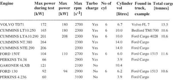
VTI has obtained emission data for 10 different diesel engines from Mr Hickman at TRL in Great Britain. These engines from the years 1985-1990 are representa-tive of the British eet of trucks (with a total weight between 7 and 38 tonnes) of those years. The engines and certain characteristics describing them are presented

in Table 1 (some basic data are from the automotive handbook Last og Buss, 1985 1990).

Table 1 Engines that have been studied during the US transient test and cer

tain related data.

Engine Max power Max Max Turbo No of Cylinder Found in Total cargo during test power rpm charge cyl vol truck, [tonnes]

[kW] [kW] [5'1] [litres] example

VOLVO TD71 172 180 2700 Yes 6 6.7 Volvo FL 7 15.5

CUMMINS LT10.250 165 180 2300 Yes 6 10.0 Bedford TM1700 10.6 CUMMINS LTA10.290 201 208 2300 Yes 6 10.0 Ford Cargo 4028 10.6

CUMMINS NT.380 264 2300 Yes 14.0 Ford Cargo

CUMMINS NTE.290 206 2300 Yes 14.0 Ford Cargo

FORD 150T 104 110 2700 Yes 6 6.0 Ford Cargo 1515 11.6

PERKINS T438 66 2900 Yes 3.9 Ford Cargo

GARDNER 6LXB 121 2100 No 10.4

FORD 130 92 94 2900 No 6 6.2 Ford Cargo 1513 10.6

PERKINS 4.236 60 3100 No 3.9 Ford Cargo

The engine data in the input files contain engine performance data and emis

sion levels for each second during the US transient test comprising 1200 seconds.

Engine data are obtained both for a cold start and for a hot start. During each

second, data are registered as shown in Table 2.

Table 2 Example of diesel engine input data. The labels. describe the content and the anitsfor the data.

Time Speed Load Air Fuel Turbo C0 C02 HC NOx Partic Smoke Smoke Coolant

temp temp

sec rpm Nm g/sec g/sec rpm mg/s g/s mg/s mg/s mg/s m-l 0C 0C 0 428 106 29.88 0.723 5160 1.743 0.124 0.000 0.00 2.674 0.04 50 59.4

1 557 -40 35.93 0.463 6180 2.905 0.311 0.000 15.35 2.44 20.05 51 59.4 559 27 36.86 0.367 6600 1.744 0.457 0.652 23.02 2.209 0.10 52 59.4

[Q

2 Scope and method

2.1 Purpose

Our aim in the current study has been to:

1. Identify correction functions for determination of appropriate emission values during transient state conditions.

2. Estimate the rpm-torque tables with emission levels of various types during steady state conditions.

3. Determine cold start effects.

A possible application of the results is in estimating exhaust emissions in the VETO model (a computer program for calculation of transport costs and exhaust emissions as a function of road standard) developed at VTI.

The emissions of interest are:

1. C02 Carbon dioxide (basically because this should be proportional to the power level)

NOX Nitrogen oxides

Part Particles HC Hydrocarbons CO Carbon monoxide 9. 43 99 !

2.2 Literature

Pollution formation in diesel engines is discussed in the basic textbook by Hey wood [1988]. One important parameter for NO formation (which leads to NOX exhaust emissions) is the crank angle when ignition occurs, where early ignition gives higher values. N0 formation is inversely proportional to the ame tempera-ture that varies with the amount of dilutants (e.g. exhaust gas and nitrogen) and oxygen. Dilutants reduce the temperature and oxygen increases it.

The formation of particles during operation of a diesel engine is a very compli-cated process. Theoretically, the soot oxidation rate increases with the oxygen partial pressure and decreases with the reciprocal temperature, where low temperatures are more important than the oxygen pressure (pages 643-645). The point in the engine cycle at which the soot-laden burned gas mixture passes through stoichiometric conditions is very important. For the late fuel-air mixing elements (at 400 crank angle) that are mixed lean of stoichiometric conditions, the carbon mass oxidised is approximately 50 % of that for the early mix (close to a crank angle 2 0°). This is essentially caused by the decreasing gas temperatures as the expansion stroke proceeds.

Hydrocarbon emissions from diesel engines are primarily caused by:

1. Fuel that is mixed leaner than the lean combustion limit (fuel to air

equiva-lence ratio ¢=(F/A)actual/(PIA)stoichiometsz.3) during the ignition delay

period. The emissions increase exponentially with the ignition delay, which depends on the actual operating conditions, such as the amount of fuel injected, the mixing rate with air and the extent to which cylinder conditions are conducive to autoignition. Overmixing is especially important at light loads and idling.

2. Undermixing of fuel leaving the fuel injector at low velocity late in the combustion process. This is important under transient conditions (accelerations). When increasing the injected fuel at a constant speed, with VTI rapport 408A

ignition delay adjusted to its minimum value, the HC emissions are initially unaffected by the increasing fuel to air equivalence ratio, but when this ratio reaches a critical value of approximately 0.9 the levels increase dramatically.

Carbon monoxide is controlled primarily by the air to fuel ratio (A/F) according to a single curve (starting at a high value for a low relative A/F-value

(k=(A/F)actual/(NF)Stoichiomemc 2 0.6-0.7) and decreasing linearly to a low value from the point when the A/F-value (kzl ) corresponds to stoichiometric combustion,

see page 592), but is considered low enough to be unimportant.

Herzog [1976] has used valid emission and engine data for stationary condi-tions, and introduced correction functions based on the changes in the relative air to fuel equivalence ratio, 7t. The approach gave computed results close to empi-rical data from some transient driving cycles. Emission data for three "generations" of diesel engines, naturally aspirated, turbocharged and turbo-charged/aftercooled were studied by Sams et al [1992] during the US transient test.Comparisons of emissions from the US transient test with simulations using emission data for stationary conditions showed the following (deviations are given

with simulated data as the baseline):

1. A reduction in NOX emissions of 20 % for the turbocharged engine, while

the other two gave almost identical results.

2. Increases in particle emissions of between 20 and 60 %. 3. Approximately the same C02, HC and CO emissions.

Analysis of engine data, such as those from TRL, raises the important question

of whether the data are in phase. Jost et a1 [1992] has developed a method for

off-set analysis, "Viruelle Zeitverschiebung". The method involves a classification of input data in a torque rpm matrix.

Then the average standard deviations of the emission levels over all matrix

elements are calculated for different constant offsets, and the offset minimising the standard deviation is chosen. A correction function for transient driving is de termined by computing average differences between data from transient and sta tionary conditions respectively for all classes of torque and rpm levels. These average differences together with the stationary data are used to construct the torque-rpm matrix of interest.

2.3 Method

When studying plots of emission levels together with the power levels, there is obviously in many cases an offset in the observations due to varying exhaust ow rates caused by the engine load variation during the test. This is discussed in more detail in Section 3.1. A method for dynamically adjusting the offsets (DOAM) is presented and examples of the results are shown.

The apparent closeness of the plotted, normalised C02 and NOX emission levels to the plots of the normalised power level suggests the use of a simple linear regression model for explaining the emission levels. Application of linear

regression models is discussed in Section 3.1. Recognizing the strong dependence

between the NOX and C02 emissions on the power level led to the formulation of a non-linear regression model encompassing power functions of the torque and rpm levels, and exponential functions for the first order derivatives (numerical

estimates) of the torque and rpm levels (Section 3.3). This non-linear model is used for establishing a measure of the prevailing transient effects.

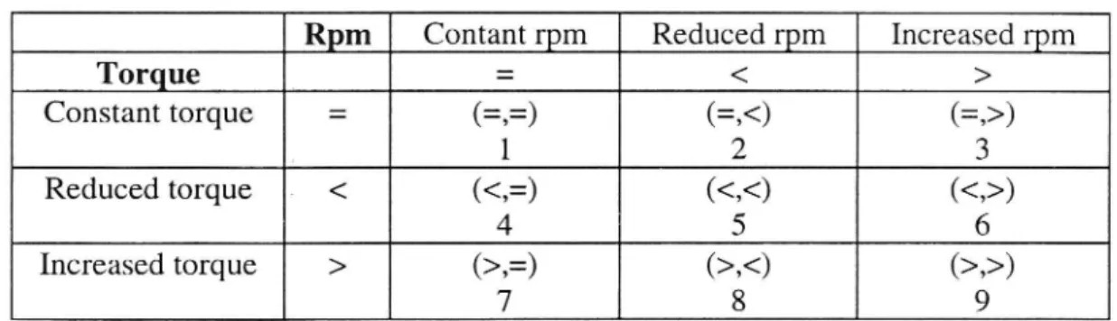
In an attempt to identify the effects during transient states, using a very diffe rent aproach, we have divided the observations into a nine-field table as shown in Table 3. The set of observations have been divided into a number of rpm and torque level classes. Observations within each class are divided into nine sub-classes according to Table 3, where the numbers in the cells are used in the tabu

lated results.

Table 3 Classification of observations into various states.

Rpm Contant rpm Reduced rpm Increased rpm

Torque , = < > Constant torque = =,= (=,<) (=,>) _ l 2 3 Reduced torque . < (<,=) (<,<) (<,>) 4 5 6 Increased torque > (>,=) (>,<) (>,>) 7 8 9

In the current analysis, the steady state (= constant state) has been considered to

be present when the change in rpm and torque from one second to the next is less than or equal to 5 % or alternatively less than 10 (the latter is important when dealing with torque levels close to 0). The choice of 5 % results in approximately 50 % of the observations being in the steady state. All the other observations are considered to be in a transient state. However, it should be noted that during ap-proximately 50 % of the US transient test the engine runs without any load.

3 Data analysis

3.1 Offsets in input data

When studying the power curve in parallel with the emissions of C02 over time, it is obvious that there exists a time lag in the basic input data (that should not be there). This is illustrated by plotting these curves (normalised by their maximum values and multiplied by 100) for one of the engines, the Perkins 4.236, during seconds 380 to 520 in Figure 1. The power produced by the engine in period t is computed according to:

Power, =2 R * rpm/60 * torque, /1000 [kW] (1)

As shown by the curves, the variation in the emission level appears to follow

the variations in the power level fairly closely, but the emission level of C02 starts

to increase before the increase in power appears. This is explained by Mr Hickman as a consequence of the fact that the constant adjustment used for offset in the measurements does not work perfectly. The reason is that the offset varies during the transient test due to different gas ow rates and gas volumes in the exhaust system during the process.

It is natural that the C02 emissions match the power development over time since C02 is directly proportional to the fuel used for generating the power. The existence of positive C02 values in the input data also during engine braking periods (i.e. when the fuel injection is shut off), is at least partly a result of mea-surement inaccuracy including effects related to the damping of the analysing signal.

Regarding other emissions than C02, it seems natural that they are related to the C02 emissions in that they occur ("in parallel") in the exhaust gas ow. A possible reason for differences is that particles and HC have a tendency to "stick" in the exhaust system according to Mr Hickman, thus complicating the analysing signal.

[0/0] Power and emission levels in per cent of their maximum values for the PERKINS 4.236 engine 100 Power --- -- CO2 base 80 60- 40-20a Seconds -60

Figure 1 Parallel plots of power [in kW, normalised] and C02 emissions [in g/s, normalised].

[0/0] Power and emission levels in per cent of their maximum values for the PERKINS 4.236 engine

100 . I Power ,/ MI: I I I CO2DOAII I I, \I 80 ~ } I

_{I I}

-

_I

v

_-

-

_'

' '

_{I l l}

I

I ' i a

l' , II ' l

'

'

'

-

' l

' I

l

\ 60 I \ . , . ll . . . . n I l I l 1 \ l \ I I I I , I I I'l l I 'I II 'I 'l I i n l 'l'l "' I

I I ' I . I

. :\ .

l

I;

l

40 I II, II , I/ . , \I I. \ NI I. l | w \J\ - I I . I F"\\ I I \ .1 \ i \ ¥ \ n l I I \ ' I \ \ I i I I l \ I / , "l \ l | l , I 20 l I I ' ' , I \ - l I \ I l \ \ I I \ I I \ \ I \ \ \' I \ ' ' \M \ \\ I \ \r'X J I \L, L Lr WV x

O.- | I .. _ .. I . . a ___I__ _ _ -4 _s___ .__ - I" _- _ _ - a

3:30 A ()0 420 I 40 460 4 u 90 :20

. . 1 Seconds

-20

-4o

-60

Figure 2 Parallel plots of power [in kW, normalised] and o set-adjasted C02 emissions [in g/s, normalised].

These variations in offset must be properly handled in order to carry out the intended analysis. The method for offset analysis developed by Jost et al [1992]

does not account for the variations in offset over time, and did not work very well

with our US transient test data.

We have therefore developed a method for dynamically adjusting the offsets for the emissions (DOAM), particularly the C02 emissions. Its main function is to

adjust the time lags so as to obtain parallel observations, but in the case of con

secutive time lags of different lengths we obtain overlapping data or zero valued observations. The case of overlapping data results in increased emissions in those

periods. When applying this method to the case illustrated in Figure l, we obtain

the result shown in Figure 2.

The method used for offset adjustment is described below.

Dynamic offset adjustment method (DOAM)

1. Definitions: I: time period [second], I: l, 1200 E, = max [the power level in period I, O] Ema, = max, [E,]

A, = the emission level in period I V, = offset for period t

N0! = number of observations

2. Set T21, V] = O.

3. Starting from T, identify a number of consecutive time periods having values:

Ef Z 0 ] EIHCIX

The first and last periods of the selected interval are denoted T1 and T2.

After identifying T1 and T2, proceed to step 4. If no more such periods exist, we go to Step 6.

4. Determine a preliminary offset, TH E [-5, -4, . . ., 4, 5]. This is based on

computed sums of absolute differences between the two curves for different

choice of offset according to:

T2 I

HT.) = 2 IE. -A,.T,

_rzT,

The value of T,, minimising F(TU) is chosen as a preliminary offset provided

F(0)/F(T,,)-1 is larger than 0.05, 0.07, 0.09, 0.12 or 0.16, for l T.,| = 1, 2, 3,

4 or 5 respectively. Should the initial value of T0 not be accepted, trials are

made with values successively closer to zero. This rule is based on the idea that a larger offset should be motivated by a larger reduction in the sum of

deviations, F(To), as compared to an offset equal to zero.

The preliminary offsets are saved as: V, = T0 for t = T1, ..., T2

5. IF T2 < Nobs THEN T = T2 + 1

Go to step 3

OTHERWISE go to Step 6.

6. Non-assigned elements, n, of the offset vector are given the closest, earlier

assigned offset value, i.e. Vn = Vt, where t < n and Vt has been assigned a

value. Based on the offset vector V, a new vector of periods P (showing which observation to allocate to period t) is computed according to:

Pt=t+Vt

7. The P; values, due to the assignment of preliminary offsets, may consist of overlapping period values (one period value is used more than once) and of missing period values (consecutive offset values are moved in opposite directions leading to gaps, for example an offset of -2 followed by an offset of +1 leads to 3 missing periods). Because of this, the P, values are sorted in

order of ascending values.

8. Now we go through the values in P, for t = 1, . . ., Nobs and perform:

8a. Missing periods in the vector P; PH] > P,+1. Original emission values

from the missing periods are added to the emissions in the 20 periods

equally distributed around (and including) Pt and PH 1 according to the

emission profile in these 20 periods.

8b. The new vectors of emission values are all multiplied by a factor en-suring that the accumulated emission value is equal to the initial value.

End of DOAM

Since the emission levels are non-negative and closely related to the power level, it would be useful to have a non-negative measure of the power. This can be ob tained by estimating the total power produced bythe engine. For this purpose, we compute the indicated power, Eindl, by adjusting the output power, Eoum, compu-ted according to Equation (1) with:

1. The internal friction work of the engine, Eff-[6,1, and

2. The inertia moment caused by the ywheel, Ewen, .

The equations are for computing these powers [in kW] are, see Hammarstrom and Karlsson [1987, pp 38-39]:

Em, = 2 1t* rpmt /60 * torquet /1000 (2)

E)... = - (rpm,/60 *60/2000)2* 4.2 * CV

(3)

Ewen, = - ((rpm,- rpm,-/)/60) *(21t)2 * rpm/60 * {-0.321 + 0.244 *CV)/1000 (4) where

CV = cylinder volume in litres

The indicated power is computed as:

Emit: = Eout,t - Etna; - Einer,t (5) Use of the indicated power instead of the output power gives a marginal impro vement in the number of significant effects discussed in later sections of this re-port. The indicated power curve is shown in Figures 3-7 for the Perkins 4.236 engine, together with the emission curves for C02, NOX, particles, HC and CO before and after application of DOAM.

Power (indicated) and emission levels in per cent of their maximum values for the PERKINS 4.236 engine

[%1 100 Power ind ' _a 90 r ' I _{. . . . - - - CO2 base} ,\ -. _{002 DOA} 80 -I _I 70-60 M on.t l l \ I \ '6 II] I ' a I I _{It I} i 50 r .I . l _h I j . ' 'l \ I\l : . ;, I

; l.

_{i i l i}

40 5 l': a '\ _{'l E : i} .I [I :' I f -\V\ _{:' I} : K h l ti _{,' i '} 30 E In .L I, "' _{5 5' I}} . I . l _{' ' '} g ; l .i _z 20- _{l :' ' I} s I: I _{I :} l i I I. I _{a K} I . S C. . I '\ I . k."\ _. g t: \ I ' \\ ,4 '1 O } _IL } a 380 _{440 460 480} 0 Seconds

Figure 3 Parallel plots ofpower [in kW, normalised] and C02 emissions, be fore and after o set adjustment [in g/s, normalised].

PM 100 90 ~ ~} ~\ ' -. 80 z | \X x 7o 60 -50 4o 30 20 10

Power (indicated) and emission levels in per cent of their maximum values for the PERKINS 4.236 engine

Power ind - - - NOx base NOx DOAM

380 400 460 500 Seconds 520

Figure 4 Parallelplots ofpower [in kW, normalised] and NOX emissions, before and after o set adjustment [in mg/s, normalised].

VTI rapport 408A

and after o set adjustment [in mg/s; normalised].

Figure 6 Parallel plots of power [in kW, normalised] and HC emissions, before

Seconds 380 400 420 440 460 480 500 520 [°/o] 1 oo 10 -80 7o 60 --50 40 -~ ' I I I I ' I I I " ' l l l ' l ' 90 ---HCDOAM

l,

,\

Pow er ind ~ - HC base l l l l l ' l

Power (indicated) and emission levels in per cent of their maximum values for the PERKINS 4.236 engine

Figure 5 Parallel plots ofpower [in kW, normalised] and particle emissions, before and after o set adjustment [in mg/s, normalised].

Seconds 500 520 ' l l l l l ' Pow er ind - - Part base - - F artDOAM

Power (indicated) and emission levels in per cent of their maximum values for the PERKINS 4.236 engine 20

[96]

100 Power (indicated) and emission levels in per cent of their maximum values for the PERKINS 4.236 engine

Power ind 90 «~ :. I x I I _{- - - CO base} ;',' ' ' ' ' l - CODOA 80 --7o eo so

-x {

f

30 ~ . 5 . -~. ~|_ 2o ~~ \ _ . . 400 420 440 460 480 Seconds

Figure 7 Parallel plots ofpower [in kW, normalised] and C0 emissions, before and after o set adjustment [in mg/s, normalised].

The parallel plots of indicated power levels and the various emissions in Figu-res 3 7 show that the indicated power explains a major part of the variation in the

emission levels, especially for the C02 and NOX emissions. The performance of

the DOAM approach can, for example, bejudged by fitting a linear model of the emissions as a function of the power according to:

A, =b0+b,E, +8, (6)

where

A, = exhaust emission level in period t (the notation A is used for each type of

emission)

E, = indicated power level in period I St = random variable term in period I

Since the average, standard R2 terms increase after application of the method, there are further reasons for having confidence in the approach, see Table 4. The huge variations in the HC emissions that do not follow the variations in the power

level have led us to use the C02 offset values for the HC emissions.

Table 4 Average improvement in the R2 values after application of DOAM, and the corresponding average correlations chosen among, the best obtained for each engine using data before and after application of DOAM respectively.

Emission Average ratio of R2 Average ratio of R2 Average correlation values

type values before DOAM values after DOAM Best of before/after DOAM

C02 .8628 .9652 .9824 NOX .8724 .9026 .9501 Partic .6360 .6898 .8236 HC .4261 .4477 .5857 CO .4794 .4894 .6625

3.2 Regression analysis

Using the model of equation (6) resulted in a considerable variation in the R2 va-lues within the 10 engines for each type of emission, and the explanatory power of

the models is not sufficient for the HC and CO emissions in particular. Therefore a non-linear model utilising the observed linear dependence between the NOX and

' C03 emissions on the power level in a generalised manner (the values for power

and torque are highly correlated and should not both be used as explanatory vari ables in a regression model):

A[ 2 Co + cl-(Tf)c2 hf + e[

(7)

where

T,+ = max [torque level in period t, O]

n, 2 rpm level in period t

c,- = constant parameters to be determined, j = 0, l, 2, 3

By setting c2 = c3 = l and choosing suitable values for CO and c1, the results of

using equation (7) will be very similar to those obtained by using equation (6).

The option of choosing other values for c2 and c3 will enhance the possibilities of obtaining a good fit of the data.

A study of the residuals after estimating the coefficients c0 - c3, provides an op portunity to see how the other available data can be utilised. In general, it is diffi

cult to see anything other than a linear dependence on the following variables

judged to be of interest:

- difference in the torque level (a measure of the torque derivative)

- difference in the rpm level (a measure of the rpm derivative)

turbo level

difference in the turbo level (a measure of the turbo level derivative)

Therefore, a factor with an exponential function involving the differences in the

torque and rpm levels has been included in equation (8), thus having a multiplica

tive effect on the second term in equation (7). The basic formulae for determining the first order derivatives numerically are utilised.

At 2 Co + cl -(T,+)C2 .nf -exp(c4 -alT,+ +c5 -dn,) + 8t

(8)

where

de = (T; T,: .>/2

dn, 2 (nH/ - n,_/) / 2

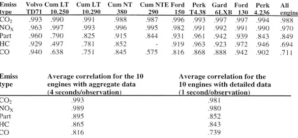
When applying this model with normalised data values, after application of the DOAM procedure (provided it led to a higher R2 value) and with the weight equal to l for each of the 1200 seconds, we obtain the correlations between the emission levels and the model values according to Table 5. Input data have been scaled so

as to avoid numerical problems in the estimation procedure; T+ and n, have been

divided by 50, and d T: and dn, have beendivided by 100.

The fact that carbon monoxide is primarily controlled by the air to fuel ratio, see Section 2.2, was tested using the air and fuel flows (see Table 2). However, it

turned out to be difficult to utilise this theoretical result, possibly a result of unreliable input data regarding time phasing and magnitude. This is especially important since the controlling variable is a ratio. Input data for utilising the other theoretical results presented in Section 2.2 were not available to us for the current

analysis.

Table 5 Correlation values for the 10 engines andfor all 10 together with the model of Equation (8) using detailed data (I second/observation).

Emiss Volvo Cum LT Cum LT Cum NT Cum NTE Ford Perk Gard Ford Perk A11

tVDe TD71 10.250 10.290 380 290 _ 150 T4.38 (SLXB 130 4.236 engi_n_e§ C02 .978 .971 .974 .969 .969 .989 .985 .992 .992 .985 .976 NOX .947 .993 .985 .990 .990 .970 .981 .982 .985 .980 .960 Part .952 .723 .733 .877 .783 .915 .937 .922 .914 .760 .817 HC .923 .455 .745 .806 - .910 .947 .901 .962 .934 .672 CO .918 .492 .622 .701 .384 .758 .842 .870 .933 .868 .670

The results of Table 5 are summarised and compared with those in Table 4 in

order to see how the average results differ. With the exception of C02, the results

when using the model of Equation (8) all give higher correlation values. Twenty seven estimated coefficients out of 324 turned out to be insignificant. One para

meter estimation did not converge (HC / engine Cum NTE 290).

Table 6 Average correlations for the 10 engines (without HC results for the Cummins NTE 290) engine.

Emission Average correlation values Average correlation values with tvpe with the model of Equation (6) the model of Equation (8)

CO; .982 .981

NOX .950 .980

Particles .824 .852

HC .634 .843

CO .662 .739

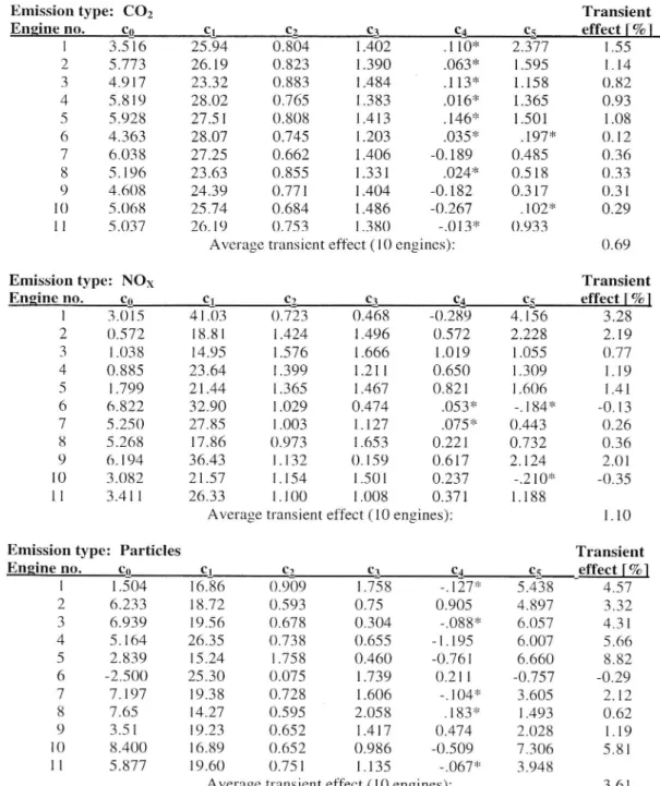
Estimated parameter values are given in Table 7 with insignificant values fol~

lowed by As can be expected, the values of c2 and c3 are in most cases bet ween O.5 and 2. Notable exceptions are the negative parameter estimates for HC and CO emissions. Positive values for c4 and c5 indicate that positive changes in

torque and rpm levels will result in increased emissions and vice versa. An unex

pected result is the fact that positive changes in the torque levels tend to reduce the emissions of C02 and NOX for some of the engines.

Prevailing transient effects for each engine are computed according to Equation

(8) with and without the transient related coefficients, c4 and c5. The transient ef-fect is then determined as: i

(Z emissions with C4 and C5)/2 (emissions without C4 and c5) ])*]00 (9)

As shown by the data in Table 7, the transient effects obtained in this way are

very small. When comparing the results for NOX and particles with experience

from engine specialists at Volvo, the results regarding NOX transients are com~ parable to theirs, but for particles we obtain only a few percentages (3.6 %) whereas their experience indicates the transient effects to be in the range 20 40 %.

Table 7a Summary ofall parameter estimatesfor model in Equation (8). Engine no. I 1 is constructed by adding normalised input datafor all engines.

Emission type: C02 Transient

Engine no. c" c, c; c3 c5 c5 effect 1%]

1 3.516 25.94 0.804 1.402 .110* 2.377 1.55 - 5.773 26.19 0.823 1.390 .063* 1.595 1.14 3 4.917 23.32 0.883 1.484 I .113* 1.158 0.82 4 5.819 28.02 0.765 1.383 .016* 1.365 0.93 5 5.928 27.51 0.808 1.413 .146* 1.501 1.08 6 4.363 28.07 0.745 1.203 035* . 197* 0.12 7 6.038 27.25 0.662 1.406 0. 189 0.485 0.36 8 5.196 23.63 0.855 1.331 .024* 0.518 0.33 9 4.608 24.39 0.771 1.404 0. 182 0.317 0.31 10 5.068 25.74 0.684 1.486 0.267 .102* 0.29 11 5.037 26.19 0.753 1.380 -.013* 0.933

Average transient effect (10 engines): 0.69

Emission type: NOX Transient

Engine no. c0 c1 c3 c3 c9 c5 effect 1%]

1

3.015

41.63

0.723

0.468

0.289

4.156

3.28

2 0.572 18.81 1.424 1.496 0.572 2.228 2.19 3 1.038 14.95 1.576 1.666 1.019 1.055 0.77 4 0.885 23.64 1.399 1.211 0.650 1.309 1.19 5 1.799 21.44 1.365 1.467 0.821 1.606 1.41 6 6.822 32.90 1.029 0.474 .053* . 184* 0. 13 7 5.250 27.85 1.003 1.127 . 75* 0.443 0.26 8 5.268 17.86 0.973 1.653 0.221 0.732 0.36 9 6.194 36.43 1.132 0.159 0.617 2.124 2.01 10 3.082 21.57 1.154 1.501 0.237 .2 10* -0.35 11 3.411 26.33 1.100 1.008 0.371 1.188

Average transient effect (10 engines): 1.10

Emission type: Particles Transient

Engine no. c9 cl c3 c3 c5 c5 _effect [%1

1 1.504 16.86 0.909 1.758 . 127* 5.438 4.57 2 6.233 18.72 0.593 0.75 0.905 4.897 3.32 3 6.939 19.56 0.678 0.304 -.088* 6.057 4.31 4 5.164 26.35 0.738 0.655 1.195 6.007 5.66 5 2.839 15.24 1.758 0.460 -0.761 6.660 8.82 6 2.500 25.30 0.075 1.739 0.211 0.757 0.29 7 7.197 19.38 0.728 I 1.606 -. 104* 3.605 2.12 8 7.65 14.27 0.595 2.058 .183* 1.493 0.62 9 3.51 19.23 0.652 1.417 0.474 2.028 1.19 10 8.400 16.89 0.652 0.986 0.509 7.306 5.81 11 5.877 19.60 0.751 1.135 .067* 3.948

Average transient effect (10 engines): 3.61

Table 7b _{Summary of all parameter estimates for model in Equation (8). Engine} no. 1] is constructed by adding normalised input data for all engines.

Emission type: HC _Transient

Engine no. (:9 c1 c: c3 c5 c5 effect [%1

1 4.435 28.26 0.111 0.928 0.698 4.516 1.75 2 18.829 0.01 -0.254 9.902 -3.539 17.009 0.51 3 24.414 0.40 -0. 151 6.631 1.080 5.197 0.27 4 16.423 1 1.02 0.083 1.73 .203" 1.996 -0.07 D - - _ - _ _ 6 14.046 23.35 0.216 0.974 0.823 1.731 0.55 7 5.107 33.22 0.096 1.165 066* -.334* 0.08 8 15.620 14.49 0.083 1.729 1.218 5.760 1.28 9 7.882 29.69 0.173 1.104 0.600 1.935 0.55 10 1628* 35.78 -0.016 1.067 0.273 2.878 0.15 11 7.084 23.25 0.019 1.035 0.327 2.356

Average transient effect (9 engines): 0.54

Emission type: CO Transient

Engine no. c9 cl c3 c3 cg c;_ _effect[%]

1 4.735 7.00 1.723 2.929 0.376 3.029 1.69 2 14.546 4.00 2.464 -.056* -3.959 11.698 3.83 3 7.157 9.95 3.083 -1.584 -1.016 11.579 10.75 4 6.690 20.09 1.319 -.092* -3.801 7.535 9.20 5 17.202 8.98 0.969 .112" 5.332 8.544 4.52 6 17.856 7.73 1.552 0.92 1.192 8.141 2.74 7 11.068 19.03 1.314 0.299 0.413 4.555 2.48 8 12.536 14.99 0.281 1.921 0.281 2.579 0.70 9 10.932 18.14 0.253 1.800 0.889 3.048 0.89 10 10.352 12.34 0.666 1.876 .186* 5.173 2.96 11 11.729 ' 15.15 1.034 0.724 -0.933 5.730

Average transient effect (10 engines): 3.98

In an attempt to overcome the problems of data that are not properly in phase,

the data have been aggregated by using averages during time intervals of 4 seconds (for the torque levels non-negative values only have been used). This in-creases the amount of correctly time phased data, but it also leads to a smoothing

of the transient effects. Since the time intervals are relatively long, the torque and rpm changes used are determined as the differences between consecutive periods

according to:

dTr+ : Tz+ Tr:

dl/lf : l lf " 74-]

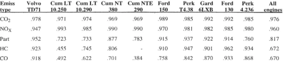
in this case. As shown in Table 8, the correlations are improved in all cases. The estimated coefficients are presented in Table 9 in the same manner as in

Table 7 with insignificant values followed by "*". In this case, 42 parameter esti

mates out of 318 turned out insignificant, which could be expected due to the

re-duced number of observations. The values for to be c2 and c3 are very similar to those in Table 7, but the values of c4 and c5 have, as can be expected, lower abso

lute values. Furthermore, the latter parameter estimates have also changed sign in

a number of cases. Estimated transient effects are fairly close to those shown in Table 7.

Table 8 Correlation valaes for the [0 engines and for all 10 together with the model of Equation (8) using aggregated data (4 seconds/obser

vation).

Emiss Volvo Cum LT Cum LT CumNT Cum NTE Ford Perk Gard Ford Perk All

tvpe TD71 10.250 10.290 380 290 150 T438 6LXB 130 4.236 engines C02 .993 .990 .991 .988 .987 .996 .993 .997 .997 .994 .988 NOX .963 .997 .993 .996 .995 .982 .991 .992 .991 .990 .970 Part .960 .790 .825 .915 .844 .931 .961 .942 .939 .843 .849 HC .929 .497 .781 .852 .919 .963 .923 .972 .946 .694 CO .940 .638 .751 .845 .575 .816 .868 .888 .942 .902 .711 Emiss Average correlation for the 10 Average correlation for the

type engines with aggregate data 10 engines with detailed data (4 seconds/observation) (1 second/observation) C02 .993 .981 NOX .989 .980 Part .895 .852 HC .865 .843 CO .816 .739

One possible explanation for the frequent occurrence of negative valuesfor c4 and 05 could be that the variables aimed at explaining the emissions under sta-tionary conditions, Tf and nt, are estimated simultaneously with the variables

aimed at explaining the emissions in transient states, dT,+ and dn,. A possible

way of dealing with this would be to use a two step procedure whereby the

coef-ficients c0 - c3 were estimated on the basis of emission data under stationary con-ditions in the first step. The values of c4 and c5 could then be determined by using

transient data. Another important explanatory factor is obviously that some data are not in phase.

Table 9a Summary of all parameter estimates for model in Equation (8). Engine no. 11 is constructed by adding normalised input data for all engines.

Emission type: C02 Transient

Engine no. c9 Cl c2 c3 c3 c5 effect 1%]

1 2.528 31.23 0.838 1.131 -0.262 0.243 0.01 2 4.484 31.47 0.845 1.156 0.246 080* 0.65 3 3.885 28.19 0.899 1.229 0.259 024* -0.91 4 4.448 33.5 0.799 1.161 -0.260 -.047* 0.99 5 4.635 32.03 0.816 1.229 0.179 .077* -0.32 6 3.681 29.81 0.743 1.108 -0.069 0.170 0.31 7 5.11 1 28.71 0.676 1.327 0.074 0.237 0.45 8 4.533 25.85 0.859 1.191 -0.091 0.188 0.17 9 3.821 26.59 0.763 1.278 0.111 0.132 0.07 10 4.061 27.86 0.675 1.364 -0. 160 0.297 0.59 11 3.971 29.56 0.763 1.213 0. 157 0.162

Average transient effect (10 engines): 0. l3

Emission type: NOX Transient

Engine no. c0 cl c; c3 c5 c5 effect 1%]

1 2.199 45.08 0.753 0.342 . 140* 0.600 1.45 2 0.483 21.95 1.395 1.288 .013* .033* 0.23 3 0.923 17.43 1.519 1.472 0.068 ~.108* 0.01 4 0.700 27.09 1.368 1.040 .018* 0.154 -0.52 5 1.649 24.27 1.343 1.305 052* -. 100* -0. 12 6 6.138 37.88 1.023 0.288 0. 198 . 175* 1.51 7 4.707 31.44 1.031 0.954 0. 158 -.089* -1.08 8 4.642 21.38 1.007 1.379 0. 169 -0.151 -1.17 9 5 .487 40.03 1.098 034* 054* 0.356 1.68 10 2.560 25.45 1.128 1.266 0. 182 -0.161 1.49 11 2.966 30.1 1 1.099 0.815 0.089 .041*

Average transient effect (10 engines): 0.25

Table 9b Summary of all parameter estimates for model in Equation (8). Engine no. I I is constructed by adding normalised input data for all engines.

Emission type: Particles Transient

Engine no. c9 cl c2 c3 c5 c5 effect 1%]

1 .996* 17.61 0.873 1.747 078* 0.884 3.92 2 3038* 19.55 0.360 0.829 0.576 1.395 5.72 3 1904* 21.38 0.285 0.445 0.404 2.503 8.74 4 2.811 32.37 0.616 0.391 0.394 2.034 5.71 5 1 . 148* 19.08 0.994 0.383 0.427 2.147 14.39 6 .296* 23.66 0.146 1.871 -.068* 1. 158 2.00 7 5.459 22.62 0.655 1.388 .133* 1.210 3.38 8 5.673 17.17 0.553 1.845 .015* .120* 0.26 9 1285* 22.16 0.524 1.272 059* 0.682 2.68 10 4.223 21.42 0.327 0.714 -.050* 2.811 8.96 1 1 3.966 22.38 0.610 1.006 005* 1.246

Average transient effect (10 engines): 5.18

Emission type: HC Transient

Engine no. c9 c1 c_2_ c3 c5 c5 effect [%]

1 6.414 25.45 0.146 0.978 0.332 1.142 2.49 2 18.904?" 0.0004* -.239* 14.521 * -1.963* .064* 160*

(estimation procedure did not converge for engine no. 2)

3 24.890 0.12 0. 154 8.782 .394* -1.805* 0.60 4 19.232 7.53 0. 1 16 2.302 0.497 -. 174* 0.69 5 _ _ _ _ .. - ._ 6 14.151 24.83 0.285 0.809 .137* -.053* 0.15 7 8.094 28.54 0.127 1.321 0.120 056* 0.16 8 15.573 14.83 0.111 1.636 0.493 1.271 1.85 9 9.799 26.57 0.226 1.162 0.300 0.525 1.50 10 5860* 30.66 0.023 1.232 0.280 0.594 0.24 11 9.633 19.71 0.018 1.191 0.288 0.677

Average transient effect (9 engines): 0.88

Emission type: CO Transient

Engine no. c9 cl c3 c3 c3 Ci effect 1%]

1 4.352 9.65 1.709 2.442 0.517 0.909 1.74 2 13.082 13.84 1.129 -1.553 2.611 5.545 4.26 3 4.686 30.67 1.180 2.463 1.179 5.793 13.17 4 4.456 37.58 1.016 -1.258 2.514 4.491 9.32 5 16.671 13.67 1.052 -1.833 4.065 6.696 6.96 6 17.685 7.54 1.270 1.015 -.302* 3.648 5.23 7 9.737 22.4 1.000 . 197* .09 1 * 1.757 4.12 8 12.293 14.81 0.355 1.863 .103* 1.180 2.31 9 11.147 17.28 0.319 1.821 0.322 0.622 1.79 10 9.300 12.5 0.538 1.865 .116* 1.999 5.57 11 10.071 19.96 0.768 0.370 0.626 2.550

Average transient effect (10 engines): 5.45

3.3 Torque-rpm diagrams

This section deals with the analysis of observations divided into a 3 by 3 matrix,

due to changes in torque and rpm levels (cf Table 3). Such a matrix hasbeen constructed for the resulting emissions, with the observations further divided into

a number of classes depending on the rpm and torque levels. For all engines the rpm class limits have been:

100 300 500 700 900 l 100 1300 1500 1700 1900 2100 2300 2500 2700 2900 3100

The torque classes have been split into a maximum of 10 classes with class widths of 50, 100, 150 or 200 depending on the minimum and maximum torque

levels during the US transient test. One of the classes has been centred around 0.

The null hyphothesis is that the expected values are equal in the nine different cells of Table 3. Within each class of rpm and torque values with at least two

ob-servations in the state (=,=) and at least two obob-servations in any of the transient

states, pairwise t tests have been performed for testing whether the emission levels violate the null hyphothesis on the 5% level (06 =0.05). Since any deviation can be

either positive or negative, a two-sided t test has been used. This means that the

cumulative t distribution' value for the test variable either should be below 06 /2 or above 1-06 /2 in order to indicate that the null hyphothesis is not true. The test

values have been computed according to:

E[xi] E[x,]

(n,-1)s3+(n, -i)s,2 _1_+i

ni+nl 2 n, 111

where

(10)

E[xi] = mean value of the observations in cell 1' (according to the notation in Table 3)

si = standard deviation for the observations in cell i ni = no. of observations in cell i

In order to handle the problem of multiple statistical inference, a procedure

suggested by Holm [1979] for identifying the significant differences has been used. Given a desired significance level of 06 and k pairwise tests are to be

per-formed, the test values are arranged according to descending values from Student's t distribution (= ascending 06 -values). For this purpose, we introduce:

F(x,r) = the cumulative probability density of Student's t distribution with the test value x and appropriate degree of freedom r

The ordered set of test values satisfies the relations:

F(lxm ,rm) 2 F( xm ,r[,]) 2 F(lxm ,rm) 2. . . 2 F(lx[k_1]l,r[k_l]) 2 F(lxwl, rm) (11)

where

lxml = the absolute value of the test value that gives the izth highest F value rm = the degree of freedom for the test that gives the izth highest F-value The reason for using the absolute values is the symmetrical property of the t

distribution.

Now the ordered F-values from equation (ll) are compared with the values 1-(X/(Zk), l oc/(2(k 1)), ..., l-OC/4, l a/Z according to Table 10.

Table 10 Ordered F-valuesfrom the tests. Position F -value Compare with

1

quml, rm)

l a/(Zk)

2

F([x[,] ,rm)

l a/(2(k-l))

k l

F('x[k_l] r[k_1])

l-a/4

k

F(lx[k] ,rm)

l oc/2

From this ordered set of F values we pick out, from the top, all the tests in the

positions where the F-value is greater than or equal to the value in the rightmost column. At the first Occurrence of a non-satisfied test, say in position q, we stop.

Now the tests in the positions 1 to q-l are significant at the level 05 regarding

errors of the first kind for any combination of true hyphotheses.

Within each rpm torque class, these tests can be performed for differences in

one type of emission individually, and for testing differences of all types of emis

sions simultaneously. Suppose that we have at least two observations in cell 1 and

p other cells of Table 3. Then the value of k in Table 10 is equal to p when testing emission levels individually and 5 *p when testing them simultaneously.

3.3.1 Description of the results

As a result of the analysis according to Section 3.3, we obtain aggregate results of

the significance tests performed in the following format (words in italics here are

only explanations), here for the Volvo TD7l engine:

No. of significances for each (significancesfor individual tests only)

emission type: 12

Total no. of significances (significancesfor both individual (both indiv and simult): 31 and simultaneous tests )

No. of rpm and torque range

combinations: 135

No. of range combinations with

at least two obs in class (=,= : 27

No. of range combinations with significant deviations: 19

No. of significant outcomes and their distribution (a positive number in any of the cells indicates the number of significant positive di erences, and a negative number the number of significant negative di erences, over all the rpm-torque class combinations. Both positive and negative di erences can appear in the same cell).

to

CO HC NO

Part 1 1

No. of Student's No. of positive No. of negative Percentage t test comparisons differences differences significances

255 21 10 12.2

Printout of deviations up and down from the mean value in each range (number

of values in the transient states over and below the steady state mean values in column 1, positive numbers indicate a positive di erence and vice versa)

2 3 4 7 < > = = to = < < > CO 17 8 8 -18 20 -5 10-16 HC .1 13-12 12 14 NO -1 20 -5 8 -18 Part 1 14 10 6 -18

The corresponding results for the other nine engines are similar to the above

figures. As an aggregate measure of success with this analysis, the numbers of significant differences for the 10 diesel engines are presented in Table 11. As

shown, the differences are both positive and negative, and in summary the results do not support the existence ofprevailing transient e ects in the engine data. This

may, however, rather be a consequence of the technique used for the analysis or some other factor in uencing the results.

Table 11 A summary of the numbers of Significant differences Obtained when applying the t-tests.

Engine No. of Student's No. of positive No. of negative Percentage t-test comparisons differences differences significances

VOLVO TD71 285 21 10 10.9 CUMMINS LT1025O 145 11 14 17.2 CUMMINS LTA10290 195 18 11 14.9 CUMMINS NT.38O 140 11 7 12.9 CUMMINS NTE.29O 185 14 7 11.4 FORD 150T 230 34 14 20.9 PERKINS T438 260 14 16 11.5 GARDNER 6LXB 210 27 12 18.6 FORD 130 250 30 14 17.6 PERKINS 4.236 215 21 12 15.3

4 Summary of results

4.1 DOAM

In Section 3.1 a procedure, DOAM (Dynamic Offset Adjustment Method), for

synchronising measured engine power levels with measured emission levels is presented. The results when applying DOAM are illustrated in Figures 3-7. Table 4 contains the resulting improvement in RZ-values when trying to explain the

emissions with a linear model including only the power level as the explaining

variable (see Equation (6)).

4.2 Exhaust emission maps using non-linear functions of

torque and rpm

Regression analysis was applied in Section 3.2 with a model including torque and rpm levels and numerical estimates of their first order derivatives (see Equation

(8)). The results obtained show high correlations between measured emission levels and model values for C02 and NOX emissions in particular, and fairly high

for particles and HC, although the estimated coefficients for the HC functions in

general appear very different from the others (with some convergence problems in the parameter estimation), see Tables 6 and 8. Models are estimated both for nor-malised input data with one observation per second, and for aggregated data with

one observation per 4 seconds. The latter case results in higher correlation values for all the cases. Transient effects are estimated with and without using the changes in torque and rpm levels (cf Equation (9)). Measured in this manner they

are fairly small, with a high level for particles that increase by 5.4 % on the

average (using aggregate data). Numerical results, estimated coefficient values and transient effects, are presented in Tables 7 and 9.

As an illustrative example, the estimated emission values of NOX from the

Volvo TD71 engine as a percentage of the maximum value during the US tran

sient test, are given in Figure 8 for relevant combinations of torque and rpm levels

(with the estimated coefficients shown in Table 7). A two-dimensional plot of the

same function for various constant relative emission levels is presented in Figure 9.

NOx&non-linearfunction Engine:1 Volvo TD71

' u u . ~ ~ c n - a a . - n 0 ~ -u ' u * - ~ - - n u . . ~ _ ~ . ~ . _. . . '. ~ ~ . . . . .u . . . ' a .

.9

'.

_{.... I}

_{/ / / /}

_{' 100}

50~'

:/

/ / /

V

5

Mn..."

l I i i I l i

5.

H

rp m [°/o]

Figure8 Relative NOX emissions under stationary conditions for the Volvo TD71 engine.

NOx emissions: lsocurves Engine: 1 Volvo TD71

90 ~~~~ - -:- - - ': - - - : - - - '

-80 . . . , . Aka . _ ,. , . . . - ._ . u u I n x . _ . . . -. . - . - .- . . . I . . . - .u . . i. . . __ 7O . . . F\\\ I 5 E 60 p ' ' ' "I' ' ' ' "I ' ' 5 _ . . . I . . . .: . . . : . - . T fm ; . . . .N . . . "In . I . . . 4O b ~ . _ . . - _ . - K: - . _ - . _ . . _ _ . , . . , ,Etmm ; . . , _ __ _ , , _ _ , _ , _ . , , . _ . . Twig; . _ . . _ . . - . 20 ' ' 'I' ' ' ' 'I' ' ' ' ' 2 ' ' _{... T ' ° ' ° ' ' ' '} 1 O l l I l I I l 20 30 4O 50 60 7O 80 90 1 00 rpm [%]

Figure 9 Isocnrves with relative NOX emissions tinder stationary conditions for the Volvo TD7] engine.

Results when computing the model coefficients with absolute emission values

according to Equation (12) (same as Equation (8) except for the scaling para-meters) are presented in Table 12 and 13. A total of 42 coefficients out of 324 turned outto be insignificant.

At = C0 + cl ("IT/500V2 ~(nt /500)"3 -exp(c4

_{/1000+c5 {int /lOO())+8t}

₍₁₂₎

where

A, = emission level in second t (the notation A is used for each type of emission) in g/s for C02 and mg/s for the other emissions

T+ = max [torque level in second t, O] in Nmf

n, 2 rpm level in second t in revolutions per minute

c, = constant parameters to be determined, j = O, l, . . . , 5

air =<T,::. Tin/2

dnf 2 ("HI Flt-l) / 2

The correlations obtained are naturally very similar to those presented in Table

5, but notable deviations in the neighbourhood of 0.1 for CO emissions in

parti-cular were observed. This is obviously caused by the varying magnitude of the

numerical values. The correlations for the 11th engine" were all lower when using the absolute values, which is natural since this engine constitutes a mix of engines

of various sizes and technologies.

Table 12 Correlation values for the 10 engines and for all 10 together with

the model of Equation (12).

Emiss Volvo Cum LT Cum LT Cum NT Cum NTE Ford Perk Gard Ford Perk All

tVDe TD71 10.250 10.290 380 290 150 T4.38 6LXB 130 4.236 engirleg C02 .976 .968 .971 .966 .966 .988 .986 .992 .992 .987 .965 NOX .945 .991 .985 .989 .988 .972 .980 .982 .984 .981 .910 Part .949 .727 .756 .887 .840 .916 .941 .918 .916 .800 .801 HC .924 .486 .791 .868 .000 .906 .947 .911 .963 .938 .508 CO .918 .586 .733 .741 .471 .810 .879 .870 .935 .880 .609 Emiss Average correlation for the 10 Average correlation for the 10 type engines with absolute data engines with normalised data

(cf Table 5) C02 .979 .981 NOX .980 .980 Part .865 .852 HC .860 .843 CO .782 .739

Table 13a Summary of all parameter estimates for model in Equation (12). Engine no. I I is constructed by adding input data for all engines. Emission type: C02 Engine no. c0 c1 c2 C3 c4 c; 1 1.073 3.38 .852 1.196 .302 .565 2 1.770 2.83 .824 1.338 029* .346 3 1.809 2.55 .888 1.422 .031* .265 4 2.966 3.66 .763 1.319 -.010* .252 5 2.368 2.98 .812 1.380 .087* .393 6 .748 2.86 .734 1.191 -.002* 049* 7 .818 2.07 .623 1.391 -.567 .219 8 1.132 2.91 .856 1.309 .094 .193 9 .825 2.22 .768 1.396 -.419 .086 10 .646 1.83 .660 1.435 1.024 088* 1 1 1.542 3.47 .992 1.207 -.045 .109

Emission type: NOX

Engine no. c0 c1 c; c; c4 c; 1 9.970 242.24 .734 .071 1.245 .688 2 2.868 37.44 1.439 1.383 .220 .231 3 5.324 23.33 1.578 1.514 .611 .286 4 5.513 38.16 1.401 1.119 .226 .189 5 16.815 49.90 1.379 1.395 .347 .223 6 24.582 228.72 1.025 .303 1.567 . 104* 7 25.857 144.06 .997 1.113 .093* .097* 8 23.372 39.13 .975 1.619 .140* .111* 9 10.889 162.56 1.089 .156 .817 .442 10 8.101 52.54 1.137 1.491 .315* 059* 1 1 14.350 63.79 .924 1.088 .373 .528

Emission type: Particles

Engine no. c0 c] 02 c3 04 c; 1 .468 1.19:" .950 1.700 .276 .974 2 1.745 2.53 .544 .880 .834 1.409 3 2.522 4.66 .672 .356 -.236* 2.131 4 2.359 5.42 .696 .610 -.634 1.947 5 1.272 7.47 1.379 .267 .618 2.176 6 .229* .65* .093 1.814 .425 .305 7 .868 102* .687 1.632 .558* .898 8 .474* 123* .180 1.967 -.410 .116* 9 .830 2.04 .584 1.460 .840 .448 10 -.032* 162* .168 .779 1.l43* 1.560 11 1.612 5.10 .926 .569 .082* 1.608

Table 13b Summary of all parameter estimates for model in Equation (12). Engine no. I] is constructed by adding input data for all engines. Emission type: HC Engine no. on cl Q C; c4 0; 1 1.363 3.47 .105 .960 .702 1.052 2 12.226 .00 -.301 9.376 3.365 5.400 3 16.613 .00 . 154 6.135 .371* -.216* 4 7.394 1.09* -.081 1.812 .626 -.074* 5 _ _ _ _ _ _ 6 4.639 3.43 .236 .998 1.141 .313 7 1.205 2.01 .118 1.211 259* .013* 8 6.665 1.56 .088 1.878 1.492 1.682 9 4.607 4.93 .204 1.187 .976 .458 10 896* 2.52 .014 1.141 1.337 -.330 1 1 -32.444 41.31 .004 .159 .090 .068 Emission type: CO Engine no c0 c1 c2 c; c4 c; 1 15.660 1.51* 1.751 3.103 .432 .514 2 17.081 28.00 1.603 - 1 . 198 3.406 3.673 3 25.61 1 267.35 1.916 -1.970 2.760 4.326 4 28.043 86.49 1.177 -.491 2.047 2.574 5 23.911 8.78 1.711 .848 -5.341 4.511 6 14.970 33.19 2.286 053* .883* 3.093 7 6.241 44.96 1.188 088* 1.614 1.695 8 1 1.249 3.65 .280 1.995 368* .859 9 8.074 2.26 .279 1.912 1.801 .586 10 8.255 2.26 .574 2.024 -.058* 1.215 11 17.330 34.68 1.345 050* -1.683 2.638

. For use in the VETO model, see Hammarstrom and Karlsson [1987], the

functions according to Equation (12) with the coefficients from Table 13 can be

used in the following manner:

1. Determine the current torque and rpm levels (T,+ and n.) and determine whether they constitue a permitted combination.

2. Determine their first order derivatives, d TL and dn, . The period should pre-ferably have a maximal length of one second.

3. Compute the exhaust emissions for each emisson type according to Equation (12).

Possibly data for a "mixed" engine obtained by weighting our input data with

respect to engine occurrence in the eet oftrucks operating in Sweden and their driving distances should be used for estimating coefficients for such an engine.

4.3 Cross tabulation

The analysis of transient effects using the cross tabulation approach and pairwise

t tests described in Section 3.3 gave inconclusive results. The established signi ficant effects turned out to be both positive and negative in the same cell of the 3

by 3 cross table, and were often so many that random effects cannot be ignored as

the probable cause. VTI rapport 408A

4.4 Cold start effects

One matter of considerable interest is the possible estimation of cold start effects based on the US transient data for diesel engines. The amounts of the five emis

sion types are computed for the entire test cycle both for the cold and hot start, where the differences are taken as measures of the cold start effects. The tempera-tures are given at the start and at the end of the test (in OC). Emissions are given in g/start and in g/kWh, see Table 14. The work performed (in kWh) is determined

according to

work = l / (1000 O 3600) 0 2 [27C 0 max[lorque, , O] 0 rpm, /60] (' l 3) In these tests the starting temperatures for a hot start are found in the range 51.9 to 76.2 0C and the ending temperatures in the range 75.7 to 95.1 0C.

Two points of particular interest regarding these data are the increase in the

C03 emissions for the FORD 130 engine for a hot start as compared to a cold start, and the fact that there are opposing signs for the cold start effect regarding C03 and fuel for the PERKINS T438 engine. The lower NOX emissions for a cold start are most likely due to the fact that the NOX emissions in general are higher at

greater temperatures.

As shown by the average values and the standard deviations, both for absolute and specific values, there are no significant effects.

Table 14 Cold start e ects for the di erent engines. Row 1: E ect in g. Row 2:

Effect in g/kWh.

Engine Start C0 C02 HC NOx Partic Fuel

temp OC [g]

[g]

[g]

[g]

[g]

[g]

cold/hot 12/l_<Wh1 [SI/kWh] 12/l_<Wh1 lg/LWhl 1R/LWh] [ lliWhl VOLVO 24.0/59.4 14.55 418.05 2.85 4.18 .13 79.17 TD71 1.31 34.69 .26 .33 .01 6.03 CUMMINS 204/633 .72 636.61 2.67 8.32 -0.32 106.35 LT10.250 .06 53.31 -0.21 ~0.66 0.02 9.17 CUMMINS 275/578 1.77 695.16 8.15 -3.69 .38 70.53 LTA10.290 0.13 47.34 .57 0.27 .03 4.52 CUMMINS 24.2/63.2 13.67 677.47 7.42 10.19 1.83 176.40 NT.380 .77 42.59 .40 0.49 .10 11.37 CUMMINS 238/762 1.03 1 172.49 1.76 -8.70 -3.67 260.48 NTE.290 .07 78.20 -0.12 ~0.61 -0.25 17.25 FORD 21 .2/69.8 11.51 265.55 2.54 -4. l3 .1 1 87.44 150T 1.68 37.59 .37 -0.63 .02 12.32 PERKINS 221/606 4.63 153.56 .20 5.74 .44 33.40 T438 .91 22.36 .03 -1.44 .08 10.98 GARDNER 249/615 9.25 291.12 3.88 7.08 1.90 166.03 6LXB 1.04 29.35 .43 .73 .21 17.72 FORD 169/519 3.34 309.36 -0.44 -3.22 .41 66.41 130 .52 -43.65 -0.06 0.45 .07 10.97 PERKINS 174/544 4.08 129.86 1.19 .79 -0.30 35.02 4.236 1.05 44.92 .33 .41 -0.06 11.82

Mean value [g/start] 6.1 413.1 2.1 -3.2 0.1 101.4 Standard deviation [g/start] 5.8 405.8 3.6 5.7 1.5 82.0 Mean value [g/kWh] 0.73 34.67 0.20 0.31 0.02 9.02 Standard deviation [g/kWh] 0.59 31.43 0.27 0.64 0.12 8.17

4.5 ECE regulation

In order to obtain emission values for these engines that can be compared with modern engines, observations have been picked out for computing emissions

equivalent to those obtained from a 13 mode test according to the ECE regulation.

For this purpose, average emission values have been computed for observed

engine data satisfying the combinations of load and rpm values according to Table

15.

Table 15 Load and rpm levels together with weightfactors for the I3-moa'e test according to the ECE regulation.

wd Rpm Weight factor Mode

Unloaded rpm at idling 0.25 1, 7 & 13

Per cent of maximum torque

100 rpm at max torque 0.25 6

75 - " - 0.08 5

50 " - 0.08 4

25 - " 0.08 3

10 - " - 0.08 2

Per cent ofmaximum power

100 rpm at max power 0.10 8

75 " 0.02 9

50 " 0.02 10

25 - " - 0.02 11

10 - " 0.02 12

Since exact matches according to the specifications cannot be made using data

from the US transient test, tolerance levels have been set so as to obtain at least

one observation for each mode (modes 1, 7 and 13 have been aggregated). Resul ting emission values have then been computed according to:

Etype = Zmode<Etype,mode*WFmode) / 2 (Pmode*WFmode)

where

Etype 2 emission of substance type in g/kWh

WFmode 2 weight factor for the various modes according to Table 15 Pmode = power level in the various modes (=2*7t*torque*rpm/(1000*3600)) As shown by the results in Table 16, the model values, with coefficients as in Table 13, are very similar to the measured data for C02 and NOX which are to be expected since the correlations are high. By looking at the bottom lines showing

the average deviations between model value and input data, we find that the model data (with input data only for stationary conditions) show an increase of 0.3 % in

C02 emissions during transient conditions (US transient) obtained as

(1/(1-0.3/100)-1)*100. Analogously, the average changes in N OX, particle, HC and CO emissions during transient conditions are -3.5, +21.8, 11.9 and +22.9 % respec-tively. However, none of the estimations is significant, as shown when comparing the averages and the standard deviations presented on the two bottom lines.

Table 16 E CE regulation data according to the de nitions of Table 15 and Equa-tion (14). Relative deviaEqua-tions between the emission levels from the US transient test and those obtainedfrom the estimated models.

C02 NOX Part HC CO Mode rpm Torquemax

LEI/kWh] lE/kWhl 12/kWh1 [g/kWhl lg/kWhl lel VOLVTD71 UST 642.8 9.16 0.45 0.45 5.75 2-6 1928 829 Model 637.0 9.16 0.45 0.51 5.58 8-12 2175 781 Dev 1%] 0.9 0.0 0.4 13.4 2.8 1,7 & 13 395 CLT10250 UST 627.2 9.85 0.42 0.55 1.67 2-6 1389 1001 Model 617.5 9.87 0.35 0.64 1.34 8-12 1874 891 Dev [ 70] l.5 0.1 l7.4 17.5 20.1 1.7 &13 512 CLT10290 UST 595.6 7.91 0.57 0.67 6.69 2 6 1377 1136 Model 607.4 8.35 0.38 0.96 3.84 8-12 1866 1036 Dev 1%] 2.0 5.6 -33.7 43.4 42.7 1,7 & 13 509 CNT380 UST 646.6 8.50 0.60 0.37 5.13 2-6 1356 1594 Model 678.5 8.84 0.45 0.49 3.74 8 12 1859 1372 Dev [%] 4.9 4.0 -24.6 31.1 27.2 1,7 & 13 462 CNTE290 UST 640.5 13.91 0.92 0.48 1.88 2 6 1317 1276 Model 650.3 14.37 0.66 0.04 1.30 8 12 1932 1030 Dev [ 70] 1.5 3.3 -27.7 - -30.9 1.7 & 13 440 FORD150 UST 622.3 12.73 0.44 0.88 1.88 2 6 1938 461 Model 627.7 13.59 0.47 1.06 2.07 8- 12 2436 424 Dev [ 70] 0.9 6.8 6.6 20.1 10.0 1,7 & 13 261 PERKT438 UST 788.0 24.79 0.58 1.05 3.80 2 6 1 183 302 Model 764.5 27.13 0.54 1.14 3.06 8 12 2510 253 Dev [%] -3.0 9.4 6.9 8.4 l9.4 1,7 & 13 516 GARD6LXB UST 656.6 12.48 0.77 1.31 2.72 2 6 1204 677 Model 637.5 12.09 0.56 1.20 2.42 8-12 1836 638 Dev [%] -2.9 -3.1 -27.3 8.4 -11.0 1,7 & 13 374 FORD130 UST 682.5 8.62 0.94 2.17 2.95 2 6 1563 385 Model 686.1 8.32 0.76 2.08 2.71 8 12 2747 319 Dev [ 70] 0.5 3.4 -l8.4 4.2 -8.2 1,7 & 13 203 PERK4236 UST 783.4 12.14 0.62 1.79 5.06 2 6 1705 258 Model 747.7 13.86 0.44 1.78 3.32 8 12 2757 213 Dev [ 70] -4.6 14.2 -29.4 -0.3 34.4 1,7 & 13 396 E[re1 deviation] -().3 3.7 -17.9 13.4 -18.7 Stand dev 2.8 5.6 13.5 16.9 16.0 [rel deviation]

4.6 Other comments on input data

When comparing the COg/fuel ratios, these are all quite far from 3.18, which is the

correct value with a carbon content in the fuel of approximately 86% (by weight). For a hot start they are found in the range [2.23, 4.01] on the basis of these engine

data, i.e. the extremes were quite far from the true value. According to Mr

Hickman, this could be explained by less accurate measurements of the fuel

con-sumption, particularly for low consumption levels.

Some observations of particle emissions have negative values according to Mr

Hickman. The explanation for this is that organic material among the particles may vaporise and vanish with the air flow through the filter in the measuring equipment. This problem occurs during periods with low emission levels in

parti-cular, but for high emission levels the procedure allegedly gives accurate

mea-surements.

5 Conclusions and future research

There are clearly time lags between the power and emission data that need to be adjusted, due to the dynamic variations in the engine load that cause variations in the gas volume flows and speeds. This is discussed in Section 3.1, and a method

for dynamically adjusting the offsets is sugggested (DOAM). _

The regression analyses carried out in Section 3.2 display good models for describing the resulting emissions of C02 and NOX, as functions of the indicated

torque and rpm levels and their variation over time. For many of the engines the models also provide good models for explaining the emissions of particles, HC

and CO. These results can be utilised for estimating the transient effects when simulating the driving of heavy duty vehicles in the VETO model, see Hammarstrom and Karlsson [1987]. Given descriptions of emissons in torque rpm

tables under stationary conditions, better estimates of the transient effects could

probably be made in the following manner:

1. Estimate steady-state functions based on test data for stationary conditions.

2. Use transient data for complementing the functions from Step 1 with mea-sures of transients.

The currently estimated models can be used, individually or aggregated, for

es-timating the transient effect given certain torque and rpm values and their first order derivatives. This result can be computed as a factor in the same manner as in

Equation (9).

Regarding the first step above, it is worth mentioning that diesel engine deve

lopers in the Swedish truck industry are promoting a new international regulation

based on measurements of emissions at all the torque and rpm levels that are frequently used in practice (1995). This is highly motivated by an attempt to avoid the possible construction of engines that meet a certain regulation but have a per formance aimed at the highest possible fuel economy in unregulated areas,

pos-sibly leading to excessive NOX emission levels, for example.

The cross tabulation of data and statistical tests of possible transients effects in Section 3.3 gave inconclusive results. There were significant differences at the 5%

level in 15 % (on the average) of all cases, see Table 11. Almost two thirds of the differences were positive. Unless it is possible to identify any logical pattern in the

results that explains the differences, our view is that the observations may serve as

a basis for emission computations during steady state conditions.

Significant cold start effects could not be detected, see Table 14. By comparing the emission levels for the case of a cold start with that of a hot start, it is possible to estimate the possible existence of increased emission levels during the cold start phase. For these engines the effect seems to be small. In connection with Table 14,

we also mention the totally unexpected increase in C02 emissions for a hot start,

which we cannot explain at this stage.

Determination of l3-mode data according to the ECE regulation shows that the

estimated models give accurate estimates of the exhaust emissions as compared to those obtained with the basic US transient data, especially in cases with high cor

relations, cf Tables 12 (correlations) and lb (ECE regulation values).

A considerable potential exists for a generalisation of these results by:

using corresponding engine data for stationary conditions and investigating

the potential of the two step procedure discussed above

analysis of engine load and emission data for typical engines in the Swedish fleet of trucks with the purpose of estimating typical emission profiles, engine maps, for various combinations of torque and rpm.

6 References

Forlaget Last 0g Buss A/S: Last og Buss; Bilteknisk oppslagstidsskrift, 1985-1990. Hammarstrom U and Karlsson B: VETO a computer program for calculation of transport costs as a function of road standard, VTI meddelande 501,

VTI, 1987.

Heywood J: Internal Combustion Engine Fundamentals, McGraW Hill, New

York, 1988.

Hickman A J: Diesel Engine Input Data (on diskettes), Transport Research

Laboratory, Department of Transport, Berkshire, Great Britain, 1992.

Hickman A J: Personal communication, Transport Research Laboratory,

Department of Transport, Berkshire, Great Britain, 1993.

Herzog P: Die Hpchrechnung instationa'rer Abgastestergebnisse aus stationaren

Kennfeldern, Osterreichische-Ingenieurzeitschrift, Vol. 19, No. 8, 1976, pp 271-276.

Jost P, Hassel D and Sonnborn K S: Neuartige Methode zur Ermittlung von Emissionsfaktoren fiir Nutzfahrzeuge, in Mitteilungen des Institutetes fiir

Verbrennungsmaschinen und Thermodynamik, Heft 64, Technische

Universitat Graz, 1992.

Holm S: A Simple Rejective Multiple Test Procedure, Scandinavian Journal of

Statistics, Vol 6, 1979, pp 65 70.

Sams T, Tieber J and Pretterhofer GzVerifizierun von Hochgerechneten Dyna-mischen Nutzfahrzeugemissionen, in Mitteilungen des Institutetes fiir Verbrennungsmaschinen und Thermodynamik, Heft 64, Technische

Universitat Graz, 1992.