On the Complexity Measurement of Industrial Control Software

(1)

M¨

alardalen University

School of Innovation Design and Engineering

V¨

aster˚

as, Sweden

Thesis for the Degree of Master of Science in Computer Science

-Software Engineering 15.0 credits

ON THE COMPLEXITY

MEASUREMENT OF INDUSTRIAL

CONTROL SOFTWARE

Adnan Muslija

ama16003@student.mdh.se

Examiner: Professor Daniel Sundmark

M¨

alardalen University, V¨

aster˚

as, Sweden

Supervisor: Dr. Eduard Paul Enoiu

M¨

alardalen University, V¨

aster˚

as, Sweden

(2)

M¨alardalen University On the Complexity Measurement of Industrial Control Software

Abstract

Embedded systems are becoming a dominant part of the computer systems that we use both in our every day life and in the industry. For domain specific and industrial use, specialized embedded systems, called Programmable Logic Controllers, are used to run software which provides supervi-sory control. Such software, also known as industrial control software, is programmed using one of the standardized IEC 61131-3 programming languages. As the size of the industrial control software increases and given that more requirements are imposed on such software, the effort and complexity of engineering software also increases. In the past decades much effort has been put into researching software complexity measures and their impact on software quality attributes such as maintainability, testability, understandability and test effort.

In this thesis we present how software complexity can be measured on industrial control software written in IEC 61131-3 Function Block Diagram (FBD) graphical programming languages. We show how software complexity can be represented on this type of software, what factors it can influence and how it can be directly measured. A set of software complexity metrics is selected and the measurement techniques adapted for the graphical syntax of FBD. These techniques are implemented in a open-source tool for software complexity measurements of FBD programs. A case study was performed using several industrial control programs from a train control management system. We have investigated the relationship between test effort (e.g., in terms of test suite size and test execution time of manually created tests) and different FBD software complexity measures. We found that there is a low but consistent correlation between software complexity measures and test effort. In particular, the FBD equivalent of Source Lines of Code metric had the highest correlation coefficient (i.e., 0.368) when compared to the test effort. Also, our results suggest that Cyclomatic complexity might not be useful for measuring the structural dimension of an FBD program and that a new structural software complexity metric might be required. The results of the correlation analysis was also used to construct a linear regression model. This model can be used as a rough estimation approach based on the software complexity measurement results. The constructed regression model might be improved by taking into account other software attributes that influence the test effort such as the program specification used for manually testing the software.

(3)

List of Figures

2.1 Two equivalent source codes written in two different program languages and paradigms.

On the left is a Java example, on the right an FBD example. . . 9

2.2 A complete and timed testing phase cycle. . . 11

4.1 The process that was used to collect relevant articles and papers. . . 14

4.2 An FBD function that outputs the square of the bigger input parameter. . . 16

4.3 Control flow graph of the squareOfBigger Java function. . . 17

4.4 Beremiz v1.2 [1] - an open source IEC 61131-3 IDE with the FBD implementation of the squareOfBigger problem. . . 19

4.5 A high-level architecture view of an examined software module D, which is used by A, B, C and is using modules E, F. . . 20

5.1 Initial architecture and functional parts of the FBD software complexity tool - Tiqva. 22 5.2 A high-level view of the input processing layer of the tool. . . 23

5.3 Graphical representation of the stereo cassette recorder. . . 24

5.4 FBD graphical program code of the Norm function. . . 25

5.5 FBD graphical program code of the Volume function block. . . 25

6.1 Number of test steps for individual test case (left) and the execution time of indi-vidual test case (right). . . 29

6.2 Normalized values for the Number of elements complexity (left) and Cyclomatic complexity(right). . . 31

6.3 A normalized area chart of two Halstead metrics (Volume and Difficulty), showing the similar distribution of said metrics across the TCSM. . . 31

6.4 Normalized values for the Information flow metric (left) and Halstead effort com-plexity(right). . . 32

6.5 Visualized predictions of the trained linear regression model. The two plots show the predictions of the model for the test effort proxy measures (number of test steps - left, test case execution time - right). . . 34

(5)

List of Tables

4.1 Halstead complexity measurement equations [2] and measurement results for square-OfBigger function. . . 18 4.2 Halstead complexity measurement results of the squareOfBigger FBD implementation. 20 5.1 Defined variables for the Norm function POU. . . 25 5.2 Defined variables for the Volume function block POU. . . 25 5.3 Software complexity measurements of the stereo cassette recorder POUs. . . 26 5.4 Software complexity measurements of the stereo cassette recorder FBD project. . . 27 6.1 Test effort measure characteristics. . . 29 6.2 Software complexity measures and the descriptive statistics of the results. . . 30 6.3 Kendall correlation coefficient (τ ) and Kendall p-value between software complexity

metrics and test effort. The test effort was expressed by two proxy values, test case execution time (E) and the number of test steps in a test case (N). . . 32 6.4 Software complexity weights, mean square error of predictions made based on said

weights and the variance score of the predictions. . . 34 A.1 Train Control Management System Test Effort expressed via Number of Test Steps

and Test Case Execution Time. . . 41 B.4 Software Complexity Measurement Results of the Train Control Management

(6)

Listings

2.1 A simple Java function that outputs 10 lines of code. Physical SLoC is 8 while the logical SLoC is 7 (blank line not counted). . . 8 4.1 A Java function that returns the square value of the bigger input parameter. . . . 16 5.1 Snippet of a Tiqva method which measures the NoE metric . . . 23

(7)

Chapter 1

Introduction

Compared to the physical counterparts that execute it, software is very abstract, and its inter-pretation and understanding can vary from person to person. While it is easier to grasp the size of a building, or the different gears of a vehicle, fully understanding what software is and what it is made of, presents a difficult task [3]. To measure software, or to measure the complexity of software, is an engineering research field that has been studied for over four decades [4] with the goal to define what software complexity is, how it can be measured and what knowledge it provides. Software complexity metrics could potentially be used to determine non-functional properties of the software. In addition, it can be used to predict other software characteristics, like the required testing effort based on the structural complexity of the software [5] or the ease of maintainability based on the size of the software [6]

Software has increased its presence in our everyday lives by being used in television remotes, smartphones, as well as in the industrial sectors. Running on computer systems called embedded systems, software is now responsible for managing the lights of a transport vehicle, opening and closing of train doors, or performing complex process controls of a power plant. One type of embedded systems used in the industrial domain are Programmable Logic Controllers (PLCs), used to execute safety-critical and operation-critical software. The domain-specific software executed on PLCs is sometimes called industrial control software. PLCs are usually programmed in one of IEC 61131-3 [7] standardized programming languages. One of the IEC 61131-3 programming languages is the Function Block Diagram (FBD) graphical programming language, which uses blocks and connections to realize a required functionality.

Software complexity metrics can be used on industrial control software. However, this has not been thoroughly researched in the scientific literature. We are not aware of any existing software complexity metrics that are used for measuring software complexity of domain-specific software written in the IEC 61131-3 FBD graphical programming language. There is a need to investigate how existing software complexity metrics can be applied on FBD programs and what changes have to be made in order to tune the measurement techniques to the FBD graphical syntax. Naturally, engineers would like to use these complexity metrics to estimate different development efficiency and effectiveness metrics. This is intuitively appealing, as these relations can be used to find a relationship between software complexity and effort needed to test the software.

In this thesis we present the adaptations needed to apply existing software complexity metrics to the FBD syntax. In addition, we present the results of a case study in which we investigated how software complexity measured can be used to estimate the test effort needed to manually test industrial control software. This software was provided by Bombardier Transportation Sweden AB and it is used for performing a wide variety of operations when controlling the train functionality. In Chapter 2 we provide the theoretical background on the concepts of software complexity measurements, IEC 61131-3 programming language standard and software testing. Related work is presented in Chapter3. In Chapter4we define the problem, present the set of software complexity metrics and software complexity measurement techniques for the FBD programming language. A tool for automatic measurement of FBD software complexity is presented in Chapter 5. The performed case study is described in Chapter 6, where we analyze and discuss the correlation results between software complexity and the test effort using several industrial control programs.

(8)

(9)

Chapter 2

Background

In this chapter, we explain the concepts necessary for understanding this thesis. The background covers three main areas of software engineering, software complexity metrics, PLCs and embedded software and software testing. The work presented in this thesis focuses on the measurement of FBD software complexity and its use as a means to estimate the necessary needed test effort.

2.1 Software Complexity Metrics

Software complexity metric is a quantitative value that describes a dimension of a software, de-pending on the type of the artifact used for measurement [3]. This statement points out two characteristics of every software complexity metric:

• A software complexity metric measures a complexity dimension of software.

• The software complexity measurement process has to be defined for a particular software artifact.

We are not aware of any universal software complexity measure that can determine all the different complexity dimensions of a software nor can it be applied to all possible software artifacts (such as the program source code or the software architecture). However, there are a number of software complexity metrics that have been used successfully in practice [8]. As shown in Listing

2.1, a simple program can be measured in terms of lines of code.

1 p u b l i c v o i d f o o ( ) { 2 S t r i n g s = ”Number : ” ; 3 i n t l i m i t = 1 0 ; 4 5 f o r (i n t i = 0 ; i < l i m i t ; i ++) { 6 System . o u t . p r i n t l n ( s + i ) ; 7 } 8 }

Listing 2.1: A simple Java function that outputs 10 lines of code. Physical SLoC is 8 while the logical SLoC is 7 (blank line not counted).

(10)

Source Lines of Code (SLoC) is a simple size metric that measures the logical (statements) and the physical (lines) size of a source file. It is a size metric, since it can only describe the size dimension of a software artifact (e.g. the program source code). The SLoC example above demonstrates how an artifact (program source code written in Java) is measured and how the results are evaluated. Some research has been performed on formal specification of software complexity metrics and properties that describe a software complexity metric [9].

Although the motivation for measuring a specific dimension of a software may vary [10], re-search done in this area showed [6, 11] that some complexity metrics may be good indicators of some quality and development effort properties. Results from the application of these software complexity measurements [4] can be used to indicate the amount of test effort required for that particular artifact or can be used to show that a software architecture has high levels of coupling [12].

In Chapter4we examine some of these metrics in more detail as well as discuss the implications of the results and how they might be of use for domain-specific programming languages as the ones used in this thesis.

2.2 PLCs and Embedded Software

Embedded software’s presence has become very dominant in most electronic devices that are used for personal and industrial use. The software running on such systems (also known as embed-ded software), can be programmed in a wide variety of programming languages. Self-contained computer systems with a CPU, RAM and IO ports called microcontrollers can be programmed using general-purpose programming languages such as the C programming language. However, for domain-specific domains (e.g. transportation, chemical industry, aerospace, automotive etc.), embedded systems called Programmable Logic Controllers (PLCs) are used to provide supervisory control [13]. In a complex system this supervisory control can be used for opening and closing doors or controlling the temperature in a furnace.

PLCs differentiate from their general-purpose counterparts in the way that they are pro-grammed, specifically the language used for programming this kind of software. While most embedded systems can be programmed using general-purpose programming languages, PLC pro-grams are usually created in one of the IEC 61131-3 programming languages [7]. IEC 61131-3 is a international standard that describes the properties and requirements for a programming language used for creating PLC programs [7]. IEC 61131-3 has a number of programming language im-plementations: Structure Text (ST), Instruction List (IL), Ladder Diagram (LD), Function Block Diagram (FBD). Two of these languages, FBD and LD, are graphical programming languages, thus they do not use the textual source code notation but rather a graphical representation (see Figure2.1).

Since the IEC 61131-3 programming languages are used in a domain-specific application, these languages have their own paradigms and best practices when it comes to embedded software development. FBD programs, which are IEC 61131-3 compatible programs, on an organizational level operate using Program Organization Units (POUs) [7]:

• Function: procedure-like program code

• Function Block: similar to Function POU with the addition of status information memory • Program: top-level program code that has access to IO ports

i f ( a > b ) { sum = a + c ; } e l s e {

sum = b + c ; }

(11)

Structured Text, the more traditional IEC 61131-3 programming language, resembles a Pascal-like program code, which results in an easy adoption of established practices and guidelines for general-purpose programming languages (e.g. Pascal best practices and guidelines). Function Block Diagrams, originally used in signal processing, are based on networks which realize the soft-ware functionality. FBD uses blocks to represent variables, operations, functions, function blocks and other IEC 61131-3 defined operators and operands. To provide a function or an operation with input parameters (variables), FBD uses connections. Connections transfer the value of a variable, a previously executed operation or function to the next block. When an FBD program is compiled to machine code, the program is evaluated from it’s exit point, meaning that the blocks in a block diagram will be evaluated based on their input connections. This means that programs will resolve every block until it reaches the input variable blocks.

Most of the properties that make up a programming language (variables, data types, functions) are also present in FBD. However, conditional statements and loops have a different approach in FBD. A Java example source code and the corresponding FBD source code shown in figure

2.1 demonstrate that difference. Although the result is same, the notion of an IF statement is encapsulated in the MAX block, and using it the FBD program performs the same function as the ST program.

Variables in FBD are initialized in a separate part of the IEC 61131-3 Integrated Development Environment (IDE). Compared to software development in Java, where all types of statements (variable declarations, function invocation and similar) can be contained in a single file and accessed in a single IDE window, FBD IDEs use the mentioned Variable window for variable declarations and a graphical programming window for the programming (as seen in Figure2.1.

Although FBD is a graphical programming language, the program content, the source code, is saved in an XML file. The XML file follows the IEC 61131-3 schema [7] for FBD programs, and is interpreted and visually displayed in an IEC 61131-3 IDE. This type of source code format enables easier parsing of FBD programs as well as extending the schema with IDE specific features.

2.3 Software Testing

An important phase of every software development process is the verification phase. Verification is the process of determining whether or not the current state of a software product fulfills the established requirements of a previous development phase [14]. One method of software verification is software testing, which is used to check if the behavior of the software is as intended (thus verifying it) and to expose faults in the software.

Software testing can be performed at different levels during software development. The software under test varies based on the level of testing: unit testing, integration testing and system testing. Unit testing is performed on a specific function in isolation. Typically, unit testing occurs directly using the code being tested and with the support of debugging tools. This type of testing might in-volve the programmers who wrote the code. Nowadays, there are many different testing techniques that are used in industry. Testing techniques can be grouped in the following main categories: ex-ploratory testing based on the software engineers intuition and experience, specification-based testing [15], Code coverage-based testing [4] and Fault-based testing. These techniques can be used in combination. For example, specification-based testing and code coverage-based testing are complementary to each other mainly because these techniques are using different test goals and sources of information.

Although these testing techniques are different, all of them employ the concept of a test case, a structured documentation of a test. A test case is defined in the IEEE Standard [16] as a set of test inputs, execution conditions, and expected results developed for a particular objective, such as to exercise a particular program path or to verify compliance with a specific requirement. A test case provides means for a software developer or software tester to create, perform, exercise and verify tests. A set of test cases, grouped together, is called a test suite and is used to test a complete feature of a software.

The testing phase can be similar for all testing levels and testing techniques, and starts with the test design step (shown in Figure2.2). This step requires collection of intended behavior require-ments, based on other software artifacts such as the documentation of the software, specification

(12)

Figure 2.2: A complete and timed testing phase cycle.

for the artifact that is tested or similar. The effort to verify the expected behavior of a software varies, and can be influenced by different properties of a software. Test effort, a measure that assigns a weight factor to the testing phase of a software, can be represented by the effort put into the individual steps of the test cycle as seen in Figure2.2 (in this case, the effort is a time variable). In other words, test effort represents the value of the resources put into the software testing phase.

(13)

Chapter 3

Related Work

Although the literature on both software complexity metrics and industrial control software written in IEC 61131-3 FBD programming language is scarce in western research databases, software complexity measurements have been researched for other graphical programming languages. The article by Olszewska, Marta and Dajsuren on tailoring software complexity metrics to Simulink models [17] describes the research on measurement of Simulink programs software complexity. The paper shows how to tailor the measurement techniques of software complexity measures to the block syntax of Simulink models and how to perform a correlation analysis between the complexity results and fault data from a Car Fuel program created using Simulink. A positive correlation was detected between components with high complexity and the number of faults. Knowledge of three domain experts has been used to validate the results, as their understanding of complexity directly relates to their results.

The lack of support for static analysis in modern IEC 61131-3 Integrated Development Envi-ronment (IDE) has been tackled by Prahofer and Ramler in their paper on the implementation of a static analysis tool for IEC 61131-3 Structured Text [18]. This paper introduces six common issues (code fault, bad smell, correct writing conventions) in software development that are also present in Structured Text. These are detected by a set of rules implemented in an extendable Java tool for automated static analysis of programs written in Structured Text. Integrating this tool with Sonar, a popular framework for static analysis of Java code, six programs are analyzed for faults in a continuous integration process.

Software complexity measurements have often been used for quantifying software quality at-tributes. Kushwaha, Dharmender Singh designed [19] a software complexity metric that would better describe testability, a common software quality attribute. This paper provided argumen-tation and evidence on how Cognitive Information Complexity Measure (CICM) captures the testability of software. CICM is explained and different properties of the metric are analyzed. CICM is used in a case study to measure complexity of a procedural C program code. A com-parison between CICM and Cyclomatic Complexity [4] is made, which points out the strengths of CICM for estimating test effort.

(14)

Chapter 4

Method and Proposed

Measurement Solutions

This chapter will serve as a roadmap through the different phases of the proposed measurement method. We will present the problem definition, the research questions based on the tackling of these problems, and the methods used to give answers to these research questions.

4.1 Problem Definition

A large number of complexity measures have been discussed in the literature for general-purpose programming languages [8] (i.e., C and Java). Different complexity and architectural component based metrics [8] (e.g., Lines of Code, McCabes Cyclomatic Metric, Halstead Metric, Information Flow Metric, McLure Complexity, Card and Glass Complexity) have been proposed to be used in practice for different programming languages. However, for domain specific programming languages used in embedded software development, contributions in the area of software complexity are limited. Based on the theoretical background from Chapter2, it is obvious that applying software complexity measurement techniques to the IEC 61131-3 FBD graphical programming language is not directly straightforward.

In addition, testing software systems is becoming increasingly difficult. Therefore, the study and development of static measurement techniques and tools to better predict the amount of effort needed to test those systems is becoming a very important field of research.

• There is a need for investigating how complexity measures can be applied to FBD software.

• There is a need to investigate how software complexity measurements can be used for estimating the test effort.

4.2 Research Questions

To summarize the defined problems and to present the problems in a structured way, the following research questions have been constructed:

• RQ 1: Which are the most relevant software complexity metrics found in the scientific liter-ature review?

• RQ 2: How to measure software complexity on FBD programs?

• RQ 3: Can software complexity metrics be used for estimating the effort needed for manually testing the FBD software?

(15)

4.3 State of the Art in Software Complexity Metrics

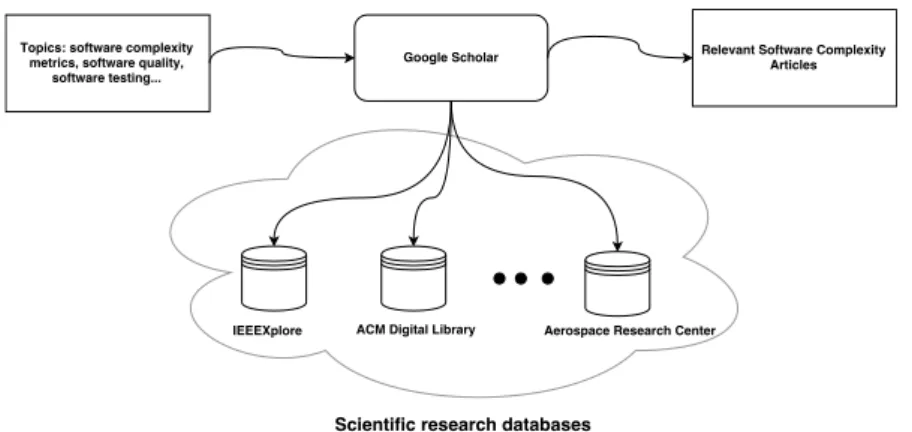
We reviewed papers and articles that focus on software complexity metrics and other software aspects that might be affected by higher or lower software complexity measures such as the testing effort, maintainability and understandability. Figure4.1displays how we used the Google Scholar search engine to filter out papers that could be relevant to RQ 1-3.

Figure 4.1: The process that was used to collect relevant articles and papers.

We initially started with papers on the general theory of software complexity which helped in capturing the details of each individual software complexity metric. One of the first papers on software complexity metrics was the original McCabe paper[4]. McCabe, using graph theory to represent program code, designed rules that are used to calculate the Cyclomatic complexity metric. This metric measures the amount of decisions that are made in the program code. Another software complexity metric that was researched during the last few decades is the Information Flow metric [12]. Kafura builds upon Hennry’s model of Information Flow theory to define a software structure complexity metric. Specific metrics are defined for procedures, module complexity and module coupling. This paper shows that this metric is appropriate for large scale systems because it is applicable at the early design phases of the system and it reveals properties regarding the system’s connections.

To formally define software complexity metrics, Weyuker [9] discussed different properties of software complexity measures and reviews popular complexity metrics based on formal definitions of software complexity properties. The paper provides proofs and examples on why some software complexity metrics describe the same properties although they measure different aspects of a software artifact. In addition, Weyuker shows some complexity metrics that do not satisfy some of these formal properties.

We reviewed papers looking in the software complexity metrics and their analysis on a higher level. Mens [3] reviewed different research trends on software complexity and previously gathered knowledge in this domain. Another case study paper [11] on the empirical study of measured software complexity metrics of two program versions gives insight into the possible expected results in this thesis. Based on the measured complexity of the programs, existing problem reports (bugs, faults, errors) as well as program reliability levels, a correlation test was performed to determine the impact of software complexity on different non-functional properties.

A similar study on the impact of software complexity measures on the maintainability of a software was performed in Kafura et al. [6] paper. Kafura analyzes the evolution of a Database Management (DBM) system developed by master level computer science students and measures its complexity and detected faults for each version of the DBM. Software complexity metrics that were measured have been grouped into code metrics (McCabe, Halstead [2]) and structure metrics (Information Flow, McClure [20]). The paper summarizes the reasons why a particular software artifact has a higher software complexity measurement results.

We used the knowledge gained from this literature review to construct a set of software com-plexity metrics that have been thoroughly researched and used in studies that focused on the correlation between software complexity measurements and other software characteristics.

(16)

4.4 A Method for Measuring Software Complexity of FBD

Programs

4.4.1 Measurement Approach and Set of Complexity Metrics

During our literature review, a significant number of software complexity metrics were discovered [4, 2, 12, 20, 21]. However, some of these metrics did not yet pass the test of time, as they were either very young or were not researched enough to be considered in papers looking at indicators of software quality and effort. We mentioned here that we did not find any relevent research done on software complexity metrics for FBD programs in the Google Scholar scientific research database. This implied that the software complexity metric set to be used in this thesis had to contain software complexity metrics that were researched in more depth by the scientific community and that some empirical evidence of their impact in practice had to exist. With this in mind, we selected a set of four metrics:

1. Source Lines of Code (SLoC) 2. Cyclomatic complexity (CC) 3. Halstead complexity (HC)

4. Information Flow complexity (IFC)

Although these metrics are somewhat conservative (since they were designed in the 70s and 80s of the 20th century), they were the subject of in-depth research and are among the most popular software complexity metrics used in the industry as well as in research [3].

Both SLoC and HC are code size metrics and can abstract the size or the length of a program artifact. The HC metric also provides information about the possible existing bugs in a software artifact or the required testing time [2] (both indicators of the maintainability of the software).

CC is a direct measure of the amount of decisions that are made in a program [4] and is often used for determining the required amount of tests for achieving basic path coverage, which can be used as a test effort measure [5].

The IFC metric proposed my Henry and Kafura is mainly used in software architecture design, since the metric computes the amount of coupling and cohesion between different software modules [12]. Although the research that we are conducting is on a unit level and not on an architecture level, FBD programs are by default very similar to other architectural models, as both architecture modeling and FBD programming is done using blocks and connections [7].

4.4.2 Source Lines of Code

We already discussed the SLoC metric as a basic example of a software complexity measure that describes the length of a software artifact, most often being a program source code. The SLoC metric is easily computed for most program source codes, as it measures a very basic property of a program - the number of program lines. However, results of SLoC measurement of two program source codes written in two different program languages cannot be simply compared, as they can be written in two different programming paradigms (procedural, functional, object-oriented).

(17)

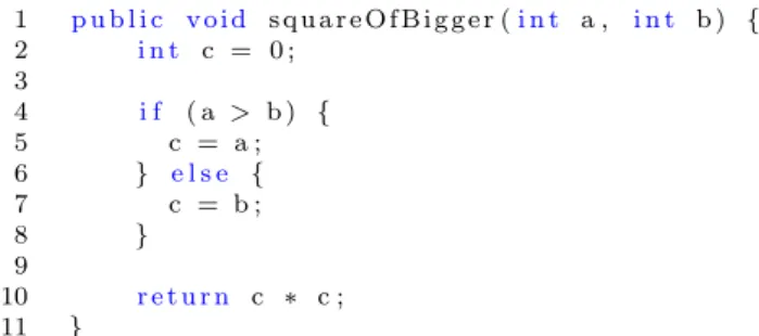
M¨alardalen University On the Complexity Measurement of Industrial Control Software 1 p u b l i c v o i d s q u a r e O f B i g g e r (i n t a , i n t b ) { 2 i n t c = 0 ; 3 4 i f ( a > b ) { 5 c = a ; 6 } e l s e { 7 c = b ; 8 } 9 10 r e t u r n c ∗ c ; 11 }

Listing 4.1: A Java function that returns the square value of the bigger input parameter. The results of SLoC measurements require some context to provide useful information, such as the reason for the measurement, the program language of the measured artifact, the expected length of the program and similar characteristics.

The Java function in Listing4.1is a very simple Java function that outputs the square value of the bigger input parameter (no specific scenario is provided when the input parameters are equal). The physical SLoC is 11, while the logical SLoC is 9 (not counting empty lines). The equivalent squareOfBigger FBD program is shown in figure4.2. It can be noticed that the technique used for measuring number of source lines from the previous Java example cannot be directly used on the FBD program.

Figure 4.2: An FBD function that outputs the square of the bigger input parameter. In the IEC 61131-3 FBD programming language, the notion of a program statement is very different compared to other general-purpose programming languages. One of the reason why this is the case is that the notion of a program statement, strictly speaking, does not exist in FBD. While in Java, a line of code can be a function call, in FBD, functions are encapsulated inside blocks. The question of how to map the SLoC metric to FBD is very similar to the questions of ”What are lines of code in an FBD program”?

If the function calls and other program statements are abstracted via blocks, and the order of their execution controlled via connections, then we can assume that SLoC metric for FBD would measure the number of blocks and connections in an FBD program. Considering that blocks and connections are graphical elements of the FBD language, and that there are other elements such as variables and data types [7] controlled by an IEC 61131-3 IDE, we could think of this metric as Number of Elements (NOE), rather than Source Lines of Code, in the context of the FBD programming language.

We propose the following steps for calculating the NoE metric for an FBD program: 1. Measure the number of variables

2. Measure the number of data types 3. Measure the number of connections 4. Measure the number of blocks 5. Sum the measured values

FBD variables can have a base type (Integer, Double, Boolean etc.) or be used as input, output or local variables, and in general, can have the same properties variables have in most programming languages (e.g. initial values, constants). FBD data types are custom data structures and have a standard FBD variable as a base structure with additional constraints [7], and can be used

(18)

as a base type of a variable. When initialized in the graphical programming environment, FBD variables and data types are represented as blocks (variable blocks), and are used as inputs or outputs for function blocks. When measuring the number of variables and data types of an FBD program, all types of variables and data types have to be included (input, output, local variables). However, their block representation in the graphical programming environment representation has to be included into the number of blocks as well.

The final result of the NoE metric is equal to the sum of individual measurements. Using previous steps we can measure the NoE metric of the FBD program shown in Figure4.2:

• Variables: 3

• Blocks: 5 (2 function blocks, 3 variable blocks) • Connections: 5

The final NoE value is 13 (sum of all FBD elements).

4.4.3 Cyclomatic Complexity

In the original paper [4], McCabe proposed a software measurement technique that measures the number if linearly independent paths through a program code. This structure metric is found upon graph theory and can be applied to a wide specter of software artifacts (from simple program functions to architectures [22]). To apply rules from graph theory, artifacts measured for CC have to be abstracted via control flow graphs.

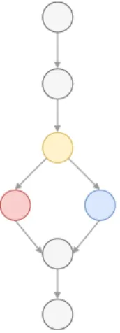
Figure 4.3: Control flow graph of the squareOfBigger Java function.

As most graphs, control flow graphs are represented via nodes and edges. A program code can be abstracted using nodes to represent program statements and edges to show the execution order of the statements, and conditional statements are presented via branching nodes. Figure4.3shows the control flog graph for the squareOfBigger 4.1 Java function. The yellow node denotes the if statement, the blue and red nodes are the two bodies of the if-else block.

The Cyclomatic complexity is defined as:

M = E − N + 2P, (4.1)

where M is the CC score, E is the number of Edges in the control flow graph, N is the number of nodes while P is the number of strongly connected components. The P usually denotes the number of exit points from a program code [4]. Using this formula and the control flow graph shown in Figure 4.3, we get a CC of 2 for the squareOfBigger function. The CC metric can be measured using an alternate equation [4]:

(19)

where Π is the number of decision points of a program and S is the number of exit points. Equation

4.2points out that the CC score is shaped by the number of conditional statements in the program. The FBD variant 4.2 of the squareOfBigger program uses the MAX block to determine the bigger of the two input parameters. The IEC 61131-3 programming language standard defines a number of different blocks that can act similarly to an if statement [7].

Since CC is influenced by the decision points of a program, the measuring technique used on programs written in general-purpose programming languages can be directly translated to the FBD programming language. Using equation4.2and the FBD example4.2we can compute aCC of 2 as well. This implies that the CC metric is less influenced by the choice of a programming language and more by the way a program is written.

4.4.4 Halstead Complexity

Compared to SLoC or CC, the HC metric [2] defines ways to compute multiple software dimensions based on the measurement of operands and operators. We assume that a set of operators for a pro-gramming language can be all the different mathematical and logical operations and propro-gramming language functions and syntax, while the set of operands of a programming language are variables and values used in the operations.

We measure the number of unique operators and operands as well as the total number of oper-ators and operands of a program to compute the proposed HC measures. For the squareOfBigger Java function4.1, following unique operators and operands occur in the function:

• Unique operators (η1): public, void, squareOfBigger, (), int, {}, =, ;, , , if, >, else, return,

*

• Unique operands (η2): a, b, c, 0

The following measurements are defined for the HC metric: Program vocabulary, Program length, Calculated program length, Volume, Difficulty, Effort, Time, Delivered bugs. Some of these measurements are computed based on the unique number and the total number of operators and operands, and the rest of the measurements are built upon them. Table 4.1 contains the equations for calculating individual HCy measures as well as the result of those measurements on the squareOfBigger Java function.

Halstead measurements Equation Result

Number of unique operators η1 14

Number of unique operands η2 4

Total number of operators N1 24

Total number of operands N2 12

Program vocabulary η = η1+ η2 18

Program length N = N1+ N2 28

Calculated program length N = ηˆ 1log2η1+ η2log2η2 61.30

Volume V = N × log₂η 116.75 Difficulty D = η1 2 × N2 η2 21 Effort E = D × V 2451.91 Time T = E_Ss, S = 18 136.21 s Delivered bugs B = E 2 3 3000 0.06

Table 4.1: Halstead complexity measurement equations [2] and measurement results for squareOfBigger function.

The HC metric aim to describe a quantitative relationship between software properties which can be measured, thus, measurements such as Volume or Difficulty describe a relationship between the measured values of operands and operators. Similar to McCabe’s Cyclomatic complexity, we observed that HC is more influenced by the syntax of the programming language.

(20)

IEC 61131-3 textual languages (Structured Text, Instruction List) resemble some general-purpose programming languages (Structured text having a similar syntax to Pascal) and HC measurement techniques are defined for such languages. Considering that the FBD language, in it’s essence, is a different approach to writing IEC 61131-3 programs, we can assume that the techniques used to measure operands and operators of a Java program can also be used to mea-sure operands and operators of FBD programs. However, FBD program variables, values and the code/algorithm itself - different operators and operands, are created in different parts of an IEC 61131-3 IDE, compared to a C program, where all the required operators and operands can be a in a single textual source code file.

Figure 4.4: Beremiz v1.2 [1] - an open source IEC 61131-3 IDE with the FBD implementation of the squareOfBigger problem.

Figure 4.4 shows the open-source IEC 6113-13 IDE Beremiz with the FBD equivalent of the Java function4.1open in it. This figure demonstrates the mentioned difference between general-purpose programming language IDE and an IDE with FBD support. POUs and DataTypes are declared in the Project frame, and the Variables and the FBD function in the main frame in the middle. The technique of measuring operators and operands can be directly applied to the Variables section of the main frame and to the DataTypes (custom data structures [7]) in the Project section. Operators like INT, Input and operands a, b can be directly measured from this IDE section, and POU and DataType operators from the Project section.

HC techniques for operators and operands is not directly defined for FBD connections and blocks, which make up the most of the FBD program and have to be measured as they directly impact the size of the program (which has been discussed in Section4.4.2).

Functions and function blocks are the different types of FBD blocks that can be found in an FBD program code. Observing the FBD implementation of the squareOfBigger function, we can deduce that operations such as comparison and multiplication are done via blocks. This implies that the different types of blocks examined in an FBD program increase the number of operations (unique and total).

Further, FBD connections do not have a direct translation such as block = function, operation, but the answer can be found if the role of connections in an FBD program is revised: the value of variables and block outputs are propagated through the FBD algorithm using connections. We already defined operands as values provided to operations and functions, thus we can conclude that connections influence the amount of operands in a program.

Using these rules, we can measure the following number of unique operations and operands: • Unique operators (η1): POU, Input, INT, MAX, MUL, function

(21)

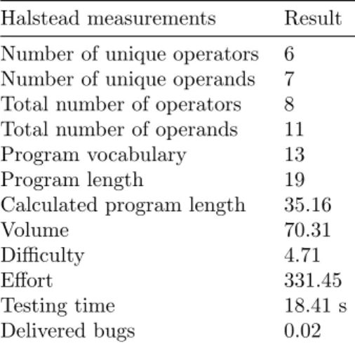
where the a-MAX and similar operands are unique connections between blocks. In this measure-ment we can also observe that the square POU function displayed in figure4.4has a default output variable with the same name, which is a characteristic of FBD POUs. The rest of the computed measurements are shown in table4.2.

Halstead measurements Result Number of unique operators 6 Number of unique operands 7 Total number of operators 8 Total number of operands 11 Program vocabulary 13

Program length 19

Calculated program length 35.16

Volume 70.31

Difficulty 4.71

Effort 331.45

Testing time 18.41 s

Delivered bugs 0.02

Table 4.2: Halstead complexity measurement results of the squareOfBigger FBD implementation.

4.4.5 Information Flow Complexity

The software complexity metrics that we examined in the previous sections are designed to measure the software complexity of a program on a unit level, to measure the complexity of functions, classes, data structures. However, other software artifacts, like software architecture and software system design also present a point of software complexity. Henry and Kafura designed a software complexity metric [12] that could be applied at earlier stages of software development, during the software architecture design.

Figure 4.5: A high-level architecture view of an examined software module D, which is used by A, B, C and is using modules E, F.

IFC of a software module provides information about the amount of coupling between the module and rest of the software system. As shown in Figure 4.5, a software module (module D) may depend on other software modules and be a dependency to others. In this example, three modules are using the examined modules, while two modules are being used by it. IFC computes a value based on those two numbers (fan-in for the number of modules using a specific module and fan-out for the number of used modules by the examined module):

c = SLOC × (fan-in × fan-out)2 (4.3)

IFC is designed to be used at a system level, but it may be used to measure the information flow between procedures or functions of a single program unit. Although IEC 61131-3 POUs (functions and function blocks) are used as program units, they can be represented as software modules in the overall software architecture of a PLC software system. Especially in FBD, a function is used as a block, thus graphically implying it’s module-like properties in an FBD program.

(22)

IFC measurement of FBD units can be simplified by measuring number of defined inputs and outputs of an FBD unit (function or function block). This provides a baseline IFC score of an FBD POU, and that value can only increase when it is used in other FBD programs.

If we examine the FBD implementation of the squareOfBigger problem in Figure 3.2, we can count two input parameters (a,b) and one output parameter (result). Considering the earlier defined properties of fan-in and fan-out numbers, we concluded that fan-in will be the number of output parameters and fan-out the number of input parameters. Thus, we can calculate the information flow complexity of squareOfBigger FBD function:

c = SLOC × (fan-in × fan-out)2= 13 × (1 × 2)2= 52 (4.4) The SLoC value was measured with the technique defined in Section4.4.2. As with the rest of the software complexity metrics that we have examined, the measurement result requires a context to provide any useful information. Thus, if compared with other FBD POUs, a POU with a high information flow complexity may be harder to maintain [11].

(23)

Chapter 5

Tool Supported Complexity

Measurement

Integrated Development Environments (IDEs) such as Eclipse [23] or IntelliJ [24] provide features for statical analysis of the software being developed. This static analysis of the code might provide information about different software complexity metrics of the given program code (e.g., SLoC be-ing a common example). Those metrics can be very useful to the developer durbe-ing the development and testing phase, depending on the context in which they are evaluated.

During the work on this thesis, we used two IEC 61131-3 IDEs: the open-source Beremiz IDE [1] and the enterprise IDE Multiprog [25]. Beremiz was already shown in Section4.4.4, with all the support for the IEC 61131-3 standard and available languages of that standard. These tools are lacking any type of software complexity measurements that some general-purpose IDEs usually offer by default.

This gave us an opportunity to design and develop a tool that would provide automatic software complexity measurements of FBD programs and report the results in a readable file format.

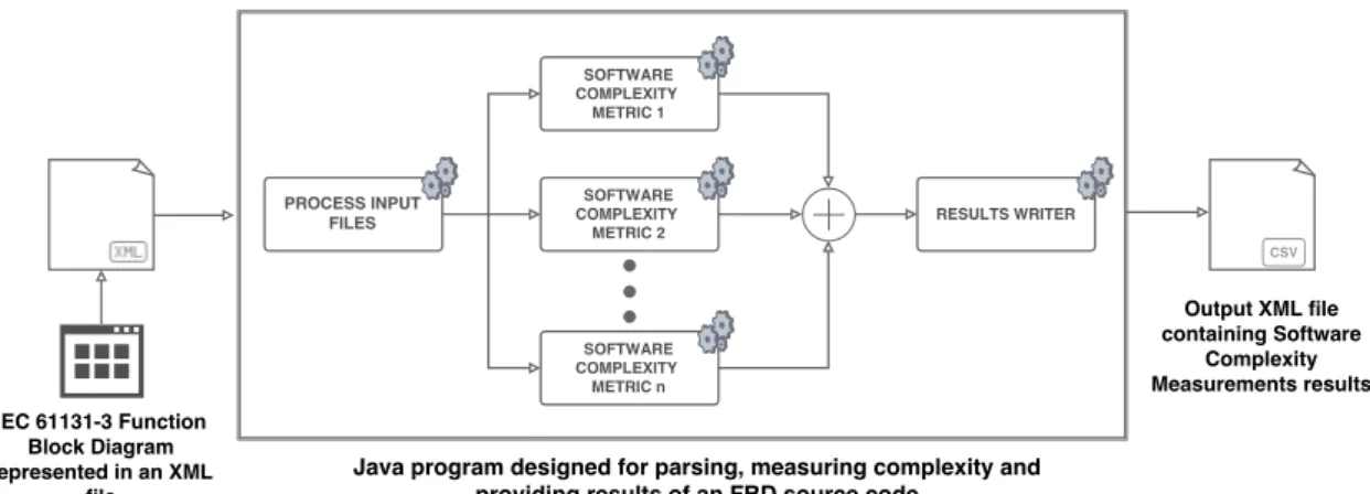
Figure 5.1: Initial architecture and functional parts of the FBD software complexity tool - Tiqva. Tiqva [26] was developed, during this thesis, as an effort create an automatic software complex-ity measurement tool for FBD programs. We decided to develop the tool in Java, as we wanted an OS-agnostic tool that could be easily used without manual configuration.

In Figure,5.1a high-level architecture view of Tiqva is shown containing three essential layers: • Processing input files: reading XML files containing FBD programs and generating a

model.

• Software complexity metrics: measuring different software complexity metrics using the earlier defined techniques and generated models.

(24)

• Results writer: Reporting the results in a machine readable file format.

Our goal is to develop a tool that could be easily added to either a continuous integration process or used independently by a developer, engineer or manager in charge of testing (thus, the requirements for a standardized input format (XML) and output format (CSV)).

Using the constructed techniques for measuring software complexity of FBD programs shown in Section4.4, we devised a set of rules for applying these techniques to an FBD file. However, applying these techniques to the XML contents of an FBD program is not convenient, as it results in complicated program code that has to deal with the XML syntax. We resolved this issue by designing an FBD data structure model that is similar to the Abstract Syntax Trees (AST) used for parsing and processing source code. The data model had to be organized hierarchically and had to be iterable as most of the techniques required iterations through an organized FBD program code.

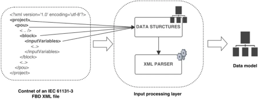
Figure 5.2: A high-level view of the input processing layer of the tool.

We mentioned in Chapter 2 that the IEC 61131-3 programming language standard provides an XSD Schema which defines the structure of an FBD XML file. The use of FBD XDS Schema rules in creation of the data model results (shown in Figure5.2) in a data model that contains all relevant program information from the FBD XML file and maintains the hierarchy and relationships between FBD elements.

The top piece of our hierarchy is the FBD Project object. A Project may have two child models, DataTypes and POUs. POUs may then have Variables, Blocks and Connections. All of the data models contain relevant information from the XML file, like the type of the object (input variable, MAX block), names, parameters and similar.

1 @Override

2 p u b l i c HashMap<S t r i n g , Double> m e a s u r e P r o j e c t C o m p l e x i t y ( P r o j e c t p r o j e c t ) { 3 HashMap<S t r i n g , Double> m e t r i c = t h i s. addKeysToMap ( ) ;

4 m e t r i c . put ( ” DataTypes ” , (d o u b l e) p r o j e c t . getDataTypes ( ) . s i z e ( ) ) ;

5 f o r (POU pou : p r o j e c t . getPOUs ( ) ) {

6 m e t r i c . put ( ” V a r i a b l e s ” , m e t r i c . g e t ( ” V a r i a b l e s ” ) + pou . g e t V a r i a b l e s ( ) . s i z e ( ) ) ; 7 m e t r i c . put ( ” B l o c k s ” , m e t r i c . g e t ( ” B l o c k s ” ) + pou . g e t B l o c k s ( ) . s i z e ( ) ) ; 8 m e t r i c . put ( ” C o n n e c t i o n s ” , m e t r i c . g e t ( ” C o n n e c t i o n s ” ) + pou . g e t C o n n e c t i o n s ( ) . s i z e ( ) ) ; 9 } 10 r e t u r n m e t r i c ; 11 }

Listing 5.1: Snippet of a Tiqva method which measures the NoE metric

To increase modularity and reusability of our tool, we created a Java interface, ComplexityMet-ric, that defines methods for measuring software complexity of an FBD program. The interface dictates two methods, one for measuring complexity of a single POU, while the other measures the complexity of the FBD project, both taking the mentioned data model objects as parameters and performing measurements on them. In Listing5.1 shows a snippet of the method used for measuring NoE scores. The snippet shows an implementation of a ComplexityMetric interface

(25)

Once the software complexity measurements are finished, the collected results have to be re-ported. The SoftwareComplexity interface methods return HashMap objects which contain the measurement results, with the name of the measurement being the map key. This makes for a con-venient and fast access of the results. For the initial version of Tiqva, we reported the measurement results in a CSV file.

Maven [27] was used for building and handling the dependencies of the tool. Tiqva depends standard Java packages found on the Maven repository. We used DOM4J framework to do the initial XML parsing, and many features of the tool depend on this framework. Since XML parsing is slow, compared to other operations that are present in Tiqva, we had to use multithreading for certain parts of the tool to compensate for the overhead introduced by the parsing. If multiple XML files are provided to the tool, each will have an individual thread for XML parsing, model building, complexity measurement. Up to 100 FBD XML projects can be parsed at a given time. Once all XML files have been measured for software complexity, the results are collected and reported using the CSV Writer.

5.1 The Measurement Approach Applied on an Example

To validate the measurement techniques that we adapted for the FBD programming language and to verify the tool for automatic analysis of FBD programs, we analyzed the stereo cassette recorder exercise and solution that was given as an example exercise in the introductory book for the IEC 61131-3 programming language [7]. The FBD solution for this problem embodies most of the the domain-specific elements of the FBD language, such as different functions, function blocks and data types.

The given requirements for the control software of the stereo cassette recorder [7] are: 1. Adjustment of the two speakers depending on the current balance control setting

(say an integer value between 5 and +5) and the volume control setting (say an integer value between 0 and +10). The amplifier output needs a REAL data type. 2. Volume control. If the volume exceeds a pre-defined constant value for some time, a warning LED must be turned on. Additionally a warning message is sent to the calling program.

3. There are two models of this recorder with different limits of loudness.

The graphical representation of the stereo cassette recorder is shown in Figure5.3and displays the hardware view of the recorder consisting of inputs (volume and balance) and outputs (left and right speaker):

Figure 5.3: Graphical representation of the stereo cassette recorder.

The problem solution contains two POUs: a function Norm and a function block Volume. The Norm function is used for normalizing volume levels, as requested in the requirements, and the Volume function block realizes the rest of the requirements. We will not go into details about the program, however we will use the FBD solution provided in the IEC 61131-3 book for software complexity measurements.

The FBD source code of the Norm function contains variables declaration and the graphical program code of the function. The variables used in this solution are shown in Table5.1and the program code is shown in Figure5.4.

(26)

ID Name Class Type Initial value

1 BIK Input SINT

2 LCtrlK Input SINT

3 MType Input BOOL

4 Calib Local CalType

5 Type1 Local REAL 6.0

6 Type2 Local REAL 4.0

Table 5.1: Defined variables for the Norm function POU.

Figure 5.4: FBD graphical program code of the Norm function.

One non-standard variable type is used in this POU, called CalType. This variable type is a custom data structure (data type) and was created as part of the cassette recorder project, and is in essence a data structure with a REAL value as it’s base type. The Norm function POU is used as a block in the Volume function block POU for normalizing input volume levels. Similar to Norm, Volume function block consists of variable declarations in Table5.2 and the graphical program code in Figure5.5.

ID Name Class Type Initial value Option 1 BalControl Input SINT

2 BalFactor Input SINT

3 VolControl Input SINT

4 ModelType Input BOOL

5 LED Output BOOL

6 Critical InOut BOOL

7 MaxVolume Local REAL 26.0 Constant

8 Timeout Local TIME 2.0

9 HeatTime Local TON

10 Overdrive Local BOOL

(27)

We implemented these programs in Beremiz and saved the project solution in the appropriate FBD XML format (the v1.01 IEC 61131-3 FBD XML structure).

Before starting software complexity measurements, we had to perform a domain-knowledge analysis of the solution, which meant understanding the standard blocks and variables as well as solution-specific blocks. Besides the CalType variable, the Norm function is used in the Volume POU, and has to be considered when measuring the CC metric, since it contains decision blocks, thus we assigned a cyclomatic weight to the block itself (similar to other decision blocks like MAX or SEL).

The initial step was the manual software complexity measurement of previously defined metrics: NoE, CC, HC and IFC. The manual measurements were verified against the measurements reported by Tiqva, with the following results reported by the tool:

Name Volume Norm

Variables 10 6

Blocks 17 11

Connections 18 10

Information flow metric 4500 243

Cyclomatic complexity 10 2 Unique operators 17 11 Unique operands 32 19 Total operators 30 18 Total operands 41 26 Program vocabulary 49 30 Program length 71 44

Calculated program length 229.49 118.76

Difficulty 10.89 7.53

Volume 398.64 215.9

Effort 4341.49 1624.96

Testing time 241.19 90.28

Delivered bugs 0.09 0.05

Table 5.3: Software complexity measurements of the stereo cassette recorder POUs. From the measurement results shown in Table5.3it can be concluded that the Volume function block has higher software complexity scores compared to the Norm function. In terms of program size, this conclusion could have been made after examining the graphical program codes shown in Figure5.5and Figure5.4. However, these are complexity measurements of individual POUs (two POUs of the Cassette Recorder FBD program), and not the complete FBD program. Compared to measuring a POU, measuring the complete FBD programs results in the aggregation of some measurement results (i.e. NoE measurements of individual POUs will be combined for the complete project). There is no obvious reason to aggregate also the CC or IFC scores, therefore we only reported the highest scores of individual POUs. The software complexity measurements for the complete FBD program are shown in Table5.4.

Some of the results reported in Table 5.4can be computed by adding together the individual results of the projects POUs, however, measurements like Unique operators and Unique operands reported in the table5.4also take into account the operators and operands occurrences found in the CalType data type.

(28)

Name Stereo cassette recorder

Variables 16

DataTypes 1

Blocks 28

Connections 28

Information flow metric 4500

Cyclomatic complexity 10 Unique operators 22 Unique operands 52 Total operators 50 Total operands 69 Program vocabulary 74 Program length 119

Calculated program length 394.53

Difficulty 14.6

Volume 738.92

Effort 10785.46

Time 599.19

Delivered bugs 0.16

Table 5.4: Software complexity measurements of the stereo cassette recorder FBD project.

Tiqva proved to be helpful addition to the measuring process, especially for very specific details of a software program (unique operators and operands). With a textbook example successfully measured for software complexity scores using the FBD techniques from Section4.4, we assumed further reported results by Tiqva as valid for further research.

(29)

Chapter 6

Case Study on the Complexity

Measurement of FBD Industrial

Control Software

In Chapter 2 we defined software complexity metrics as values that provide information about a property of a system depending on the context, which for an instance, can be the size of a software program or its structure. We developed a set of techniques for measuring software complexity of FBD programs, and used the Tiqva tool to measure the software complexity of a textbook FBD program. However, to gather more representative results, a case study on the complexity measurement of an existing industrial control software was performed.

We researched software complexity metrics on domain-specific embedded systems and software - PLCs and FBD. We used this type of software in an industrial case study to investigate the relation between software complexity metrics and test effort attributes. The safety-critical indus-trial control software we used in this case study is part of the Train Control Management System (TCMS), a system developed and used by Bombardier Transportation Sweden AB, a leading com-pany that specializes in building and manufacturing of trains and train equipment. TCMS is an embedded software running on PLCs and used for handling a wide variety of operation-critical and safety-critical functionalities of a train. TCMS is programmed in IEC 61131-3 FBD programming language, making it viable for our case study, and uses a combination the IEC 61131-3 standard function and function blocks, and in-house built function blocks.

6.1 TCMS FBD Programs Selection and Test Effort

Mea-surement

Bombardier Transportation Sweden AB provided us with 122 FBD programs from TCMS. These programs perform different operations and are in essence developed independently of each other. The measurement process would be very similar to the automatic software complexity measurement that we have performed in Section5.1. In addition, we also wanted to investigate the correlation between software complexity measures and the effort needed to test these programs.

We had access to test cases for individual TCMS FBD programs, which have been manually created and used for unit testing. These test cases are used to perform a correlation analysis between the test effort and the reported software complexity scores. This correlation could be useful to estimate to estimate the test effort.

The test effort was not measure directly and we used a proxy measure of effort. This was per-formed before proceeding with the software complexity measurements and correlation analysis. As mentioned before, test cases were designed for individual FBD programs and consisted of several test steps. We also had access to the execution time of these test cases. This implied that we could express test effort for a FBD program as:

(30)

1. Number of test steps for each program

2. Execution time of the test case for each program.

We note here, that the second test measure contains information about the first; the execution time of a test case is the execution time of individual test steps. However, we kept both of these measures because we wanted to explore any correlation and relation between test effort and FBD software complexity metrics.

From all the programs provided, 82 had test cases. This resulted in the removal of some of TCMS FBD programs from our correlation study, as they did not contained a manually created test case. We calculated the Kendall’s rank correlation coefficient as a measure of correlation between the software complexity measurements and the test effort measures. We discussed the results in Section6.3. 20 40 60 80 100 20 40 Test Case ID Num b er of test steps in test case 20 40 60 80 100 100 200 300 Test Case ID T est case execution time [sec]

Figure 6.1: Number of test steps for individual test case (left) and the execution time of individual test case (right).

We separated the test data into two sets for each test effort measure, making the Kendall correlation easier to perform based on individual data sets. A graphical representation of the sets is shown in Figure6.1, each circle representing the test effort measure for that test case. Test effort measure data outliers can be identified in Table6.1, such as the 900 seconds execution time of a test case (not shown in Figure6.1) or a test case with only 1 test step.

Test effort measure Min Max Average Median Standard Distribution

Number of test steps 1 31 8.5 6 6.236

Test case execution 1 900 32.2804 10 105.206

Table 6.1: Test effort measure characteristics.

6.2 Overall Complexity Measurement Results of TCMS

We measured different software complexity metrics of the FBD program set provided by Bom-bardier Transportation Sweden AB using the Tiqva tool that we have developed for this particular scenario. This work can be a tedious and mistake-prone job of measuring software complexity if manually performed. Although we were provided with more than a hundred programs, we selected only those who had a paired test case, as those could be used for the correlation analysis.

We discussed how similar measurements techniques and tools do not exist for the IEC 61131-3 graphical programming language FBD, resulting in a lack of tools that perform FBD software

(31)

FBD programs used in the case study (e.g. the memory size of the FBD program, number of XML lines in a file).

The software complexity measurement techniques for FBD programs discussed in Section4.4

can be broken down into smaller individual measurements, such as the measurement of blocks and connections for the Number of Elements metric. This resulted in a total of 15 measurements for all exercised software complexity measures (NoE, CC, HC, IFC). The results reported by Tiqva consisted of these 15 measurements for the selected 82 programs (shown in AppendixB).

Software complexity measure Xmin Xmax X¯ Xe std(X)

Variables 4 85 22 18.5 14.7

Connections 3 216 33.8 25.5 32.5

Blocks 5 228 39 29.5 35.1

Number of elements 12 483 94.8 74.5 80

Cyclomatic complexity 1 133 18.9 13 21.8

Information flow complexity 12 57065472 2690651 68506 8478907.8

Unique operators 8 19 11.4 11 2.64 Unique operands 9 262 59.5 47.5 47.06 Total operators 12 229 59.1 49.5 39.88 Total operands 12 402 86.3 69 71.18 Program vocabulary 17 278 71 60 48.59 Program length 24 599 145.5 117 110.13

Calculated pogram length 52.5 2168.7 413.2 309.1 385.6

Volume 98.1 4844.3 942.5 691.5 886.8

Difficulty 5.3 14.1 8.1 7.9 1.8

Effort 523.2 59747.4 8756.5 5470.9 10925.8

Time 29 3319.3 486.4 303.9 606.9

Delivere bugs 0.02 0.5 0.1 0.1 0.09

Table 6.2: Software complexity measures and the descriptive statistics of the results. The results shown in Table 6.2helped us to develop a notion of a complex FBD program and how different complexity metrics represent an industrial control software. The different software complexity measures cannot be directly compared, but most of the values are in the same order of magnitude. However, the maximal complexity value for the IFC stands out as the highest value and is one of the outliers from of the TCMS software complexity measurement. We traced these high complexity values shown in Table 6.2 to their corresponding programs, and gathered the names of programs that were the cause for these outliers.

Four FBD programs from TCMS had high software complexity scores: Program 9, Program 60, Program 32 and Program 55. In particular, Program 32 had some of the highest scores for a number of software complexity measures (Number of Elements, CC, and HC), Program 55 had the highest Number of Elements score, Program 60 had the highest IFC score and Program 9 the highest Halstead Difficulty score. Upon closer inspection, Program 32 had one of the highest number of inputs/outputs (almost as high as Program 60) and also a high Number of Elements (also close to program 55). We could identify Program 32 as the most complex program in the TCMS, but this information on itself does not indicate good or bad software qualities of TCMS.

Since we did not have any other software complexity measurements besides the ones provided by Tiqva, we did not have the information about which software complexity scores implied that a program is complex (in respect to that software complexity). We normalized the reported values to get a better look on how individual software complexity metrics are distributed over the complete TCSM program suite. Normalized value 0 represent a very low complexity while a normalized value of 1 was the highest complexity for a particular complexity measure of the TCMS.

The scatter graphs in Figure6.2shows the distribution of one size metric (Number of elements) and one structure metric (CC). The outliers can be easily detected (Programs 32 and Program 55), but the rest of the programs have half the complexity scores the outliers have. This trend can also be seen with IFC and Halstead Difficulty (this HC metric is a function of the rest of

(32)

M¨alardalen University On the Complexity Measurement of Industrial Control Software 20 40 60 80 0.2 0.4 0.6 0.8 1 Program ID NoE complexit y 20 40 60 80 0 0.2 0.4 0.6 0.8 1 Program ID Cyclomatic Complexit y

Figure 6.2: Normalized values for the Number of elements complexity (left) and Cyclomatic complexity(right).

HC measurements). IFC shown in Figure6.4 is certainly the most polarized, due the enormous difference between the median value of that complexity and the outlier. Figure6.3shows the area chart of two HCs, Halstead Difficulty and Halstead Volume, which are functions of basic Halstead measurements metrics and are used to construct the rest of the metrics (Effort, Testing Time and Delivered bugs). Both of these metrics shown in Figure6.3have a very similar shape, which could imply that HCs will have a similar distribution through out the whole industrial control software.

10 20 30 40 50 60 70 80 0.5 1 1.5 2 Program ID Halstead Metrics Volume Difficulty

Figure 6.3: A normalized area chart of two Halstead metrics (Volume and Difficulty), showing the similar distribution of said metrics across the TCSM.

A similar distribution to CC and Number of Elements can also be observed for the Halstead Effort metric. The outliers are again programs 61 and 32. The similar measurement results and the repeating outliers suggest that these complexity metrics measure the same software dimension (size) by measuring different properties.

The set of used software complexity measurements, consisting of Number of Elements, Halstead Metric, CC and Information Flow metric, contained two size metrics (NoE, Halstead), one structure metric (CC) and one architectural metric (IFC). However, we got very similar measurement results for size metrics and structure metrics. This could be an indicator that the way we measured the structural complexity of FBD programs (the proposed cyclomatic complexity technique) does not correctly capture the structure of the program, or that FBD program structure is a different type of property compared to structures of general purpose programming languages.

On the Complexity Measurement of Industrial Control Software

M¨

alardalen University

School of Innovation Design and Engineering

V¨

aster˚

as, Sweden

Thesis for the Degree of Master of Science in Computer Science

-Software Engineering 15.0 credits

ON THE COMPLEXITY

MEASUREMENT OF INDUSTRIAL

CONTROL SOFTWARE

Adnan Muslija

ama16003@student.mdh.se

Examiner: Professor Daniel Sundmark

M¨

alardalen University, V¨

aster˚

as, Sweden

Supervisor: Dr. Eduard Paul Enoiu

M¨

alardalen University, V¨

aster˚

as, Sweden

Table of Contents

List of Figures

List of Tables

Listings

Chapter 1

Introduction

Chapter 2

Background

2.1

Software Complexity Metrics

2.2

PLCs and Embedded Software

2.3

Software Testing

Chapter 3

Related Work

Chapter 4

Method and Proposed

Measurement Solutions

4.1

Problem Definition

4.2

Research Questions

4.3

State of the Art in Software Complexity Metrics

4.4

A Method for Measuring Software Complexity of FBD

Programs

4.4.1

Measurement Approach and Set of Complexity Metrics

4.4.2

Source Lines of Code

4.4.3

Cyclomatic Complexity

4.4.4

Halstead Complexity

4.4.5

Information Flow Complexity

Chapter 5

Tool Supported Complexity

Measurement

5.1

The Measurement Approach Applied on an Example

Chapter 6

Case Study on the Complexity

Measurement of FBD Industrial

Control Software

6.1

TCMS FBD Programs Selection and Test Effort

Mea-surement

6.2

Overall Complexity Measurement Results of TCMS