J
Ö N K Ö P I N GI
N T E R N A T I O N A LB
U S I N E S SS
C H O O LJÖNKÖPING UNIVERSITY
The Stock Market and
Government Debt
The Impact of Government Debt Changes on Stock Market Movements
Bachelor Thesis within Economics Author: Wendela Johanna Gerleman Tutor: Johan Klaesson, Johan P. Larsson
and Tina Alpfält Date: May 2012
Bachelor Thesis within Economics
Title: The Stock Market and Government Debt, The Impact of Government Debt Changes on Stock Market Movements
Author: Wendela Johanna Gerleman
Tutors: Johan Klaesson, Johan P Larsson and Tina Alpfält Date: May 2012
Keywords: Stock Market, Government Debt, Granger Causality Test and Efficient Market Hypothesis.
Abstract
This thesis investigates whether or not changes in a country’s government debt could affect its domestic stock market performance. The relationship is investigated by examining three different European countries, Germany, Portugal and Sweden, on the basis of two variables; (1) quarterly government debt changes as a percentage of gross domestic product and (2) the quarterly stock market changes over the time period 2000:Q2 – 2011:Q2.
The evidence is presented with help of Ordinary Least Square Method and Granger Causality test for each respective country. According to the Efficient Market Hypothesis, stock market prices should fully reflect all relevant information, e.g. government debt changes, as soon as they occur, without any delay, if the market is efficient. Past information should be insignificant and therefore not affect the stock market prices in an efficient market.
In the cases of Sweden and Germany, the results proved to be ambiguous and thus do not allow for either rejection or acceptance of the Efficient Market Hypothesis with respect to government debt changes. However, some support was found in the case of Germany since the government debt changes and the stock market performance were instantaneously correlated.
The empirical results presented in this thesis further allowed for the assumption that Portugal was not able to efficiently capture changes in the debt levels without any delay. This indicates that the Efficient Market Hypothesis can be rejected in regards for Portugal with respect to government debt changes. Furthermore, since the Portuguese stock market performance was not able to capture efficiently changes in the government debt level, it hence could possibly mislead the direction of the economy when looking into the stock prices to determine economic conditions.
Moreover, the results imply that each country faces different relationships between the variables and that the relationships possibly could depend on the economic health of a country.
Table of Contents
1 Introduction ... 1
1.1 Purpose and Research Questions ... 1
1.2 Delimitations ... 2 1.3 Outline ... 2 2 Background ... 3 2.1 Literature Review ... 3 2.2 Government Debt ... 4 2.3 Stock Market ... 5
3 The Current Economic Debt Crisis ... 6
4 Theoretical Framework ... 9
4.1 Efficient Market Hypothesis ... 9
4.2 Budget Deficits, High Government Debt Levels, and Standard Security Evaluation Model ... 10
5 Empirical Research ... 12
5.1 Data, Variables and Descriptive Statistics ... 12
5.1.1 Control Variables ... 13
5.1.2 Descriptive Statistics ... 13
5.2 Empirics ... 14
5.2.1 Ordinary Least Square ... 14
5.2.2 Robustness – Ordinary Least Square ... 15
5.2.3 Granger Causality Test ... 16
5.2.4 Robustness – Granger Causality Test ... 17
6 Discussion of Empirical Results ... 18
7 Conclusions and Suggestions for Further Studies ... 21
List of References ... 22
Appendix ... 25
Figures Figure (1) Government Debt Levels (2007:Q3-2011Q3) ... 7
Figure (2) Stock Market Performance (2007:Q3-2011:Q3) ... 8
Tables Table (1) Descriptive Statistics ... 13
Table (2) Ordinary Least Square Output ... 15
1
Introduction
The European countries’ aggregated debt levels have increased dramatically during the last decade and caused a debt crisis throughout Europe. The increasing attention paid to the subject of government debt overload in both academia and in macroeconomic policy investigates how the escalating budget deficits can have various possible effects on the economy as a whole. From both an academic perspective and real-world experience it is a valid assumption to assume that public debt overload causes instability in a country’s economic situation and nurtures doubt in investors’ confidence.
However, another variable that plays a crucial role for an economy is its domestic stock market. Stocks are traded on a daily basis and more or less the majority of a country’s population has some connections to it. Some people have their retirement funds invested in the stock market while others depend on it as their primary source of income. Thus, many people have a vested interest in the performance of the stock market.
During financial crises and recessions, the stock markets tend to perform negatively and debt levels seem to rise. Economists foresee that industrialised countries now are moving into an epoch that is characterized by higher government debt levels and lower stock market returns.
Hence, the question tendered is;
Is it possible that government debt changes affect the domestic stock market’s performance?
Verily, if true, then government debt level changes could aid the prediction of future stock market movements. When government debt is issued for investment purposes, it is expected to have a positive impact on the stock prices since it should yield future returns. On the contrary, when governments issue debt in order to finance existing debt it could have a negative impact on the stock market since it indicates that the fiscal budget does not generate enough funds to pay off previously assumed debt. To pattern a relationship between the two variables could be of great significance to predict government debt overload and to ascertain an optimal ratio of government debt to gross domestic product (GDP) where the debt changes do not have any negative impact on the stock market performance.
1.1
Purpose and Research Questions
The purpose of this thesis is to find out if countries’ government debt changes could have an impact on its domestic stock market performance, thus, if changes in government debt precede changes in the stock market.
Conclusions should be drawn from a combination of theory and empirical analyses to allow an in-depth evaluation of the relationship between the two variables. Essentially, this work will provide the reader with valuable insights into the ability of stock prices to foreshadow the instability of domestic markets as a result of government debt level changes. The conclusions will further majorly aid the clarification of the research interest and formulate answers to the three research questions at hand;
1. Do analyses allow for conclusions regarding the ability of countries government debt to influence their respective stock market?
2. Is the stock market sufficiently efficient to capture changes in government debt levels, as suggested by the Efficient Market Hypothesis?
3. Can the stock prices be used as a primary tool to evaluate a country’s fiscal economic health and its prospects with respect to government debt changes?
1.2 Delimitations
This thesis will neither investigate the magnitude of causality between the two variables government debt and stock market, nor take the amount of the aggregated debt into account. Instead, the focus is on whether the quarterly debt changes cause corresponding fluctuations in stock market prices. Moreover, if a relationship exists and this thesis provides proof of its existence, the scope of this thesis is limited in its ability to evaluate if the relationship between the two variables is positive or negative. This thesis investigates only three European countries that faced different government debt level trends during the observed period (2000:Q2 - 2011:Q2). The observed period is chosen hence the poor monitoring of quarterly government debt levels before 2000.
1.3
Outline
The next section, (2. Background) will give the reader a literature review including subjective findings to summarise existing knowledge of the topic at hand and of topics related to the issue. This background is followed by brief explanations of the two variables government debt and the stock market. The third section, (3. The Current Economic Debt Crisis) will provide the reader with a general overview of how the current recession turned into a debt crisis and the stock markets’ reactions to this situation. The fourth section, (4. Theoretical Framework) will provide the reader with economic theory to support the hypothesis of that government debt changes can affect stock market performance. The fifth section, (5. Empirical Research) will investigate the relationships empirically with help of Ordinary Least Square regressions and Granger Causality tests. The sixth section, (6. Discussion of Empirical Result) will give the reader a discussion drawn from both the theoretical and the empirical investigation. Finally this thesis will end with section seven, (7. Conclusion and Suggestions for Further Studies) were the concluding remarks are stated to answer the three research questions. The last section will also suggest topics for further studies.
2
Background
The first sub-section (2.1 Literature Review) will give a summary of existing literature of the topic and of issues related to it. The second sub-section (2.2 Government Debt) will briefly explain the concept of government debt. It is valuable to know why governments need to issue debt and the different purposes of doing so. The majority of people are familiar with the two variables government debt and stock markets, but for further clarifications a small subsection (2.3 Stock Markets) is also devoted to explain how stock market works.
2.1 Literature Review
Most of the macroeconomic literature focuses on monetary factors as the predominant indicators of the stock market returns. Fama (1981) find that stock market returns are correlated with a country’s macroeconomic factors such as inflation, interest rate, money supply and capital expenditure. Fama’s (1981) most important conclusion is that economic factors can be used to predict movements in the stock market.
Moreover, Abdullah and Hayworth (1993) studies concur with Fama’s (1981) findings, stating that inflation and growth of domestic money supply are positively related to stock market returns in the United States.
According to Arestis and Luintel (2001), one can view banks and stock markets as substitute sources for investments. Increasing interest rates have a negative effect on the stock market. Contrarily, as the interest rates decrease investors seek for higher returns on the stock market (Arestis & Luintel, 2001). The exchange rate can result in either a positive or a negative impact on stock returns. Ma and Kao (1990) suggest that for a country dominated by exports, currency depreciation is expected to have a positive impact on domestic stock market returns. Moreover, Johnson and Soenen (1998) argue that a depreciation of the currency makes imports more costly and results in a higher domestic price level, which is expected to have a negative impact on stock market returns. This however, does not correspond with the findings of Abdullah and Hayworth (1993), who find a positive relation between the two variables.
Copeland (2008) argues that the majority of macroeconomic variables are related to each other. For instance economic growth, inflation, interest rates and exchange rates can all be related in the Mundell-Fleming model and in the Dornbush overshooting model. These models imply that the variation of one variable might also result in variation of another (Copeland, 2008).
However, little emphasis was put on whether the economic health of a country’s economy is a significant factor of stock market performance. Recent academic works focus on whether a country’s economic health as measured by rating agencies has a significant impact on its domestic stock market. Research conducted by Kaminsky and Schmukler (2002), show that rating agencies’ evaluations of the economic health of emerging markets have a direct impact on the country’s domestic stock market, when the sovereign grade changes. This research also results in the identification of a spill-over-effect to neighbour countries, especially in times of crises. In contrast to the work of Schmukler and Kaminsky (2002), findings made by Brooks, Faff, Hillier, and Hillier (2004) illuminate that emerging markets show no evidence of being more vulnerable to rating changes than developed markets. Schmukler and Kaminsky (2002) argue that a sovereign downgrade, thus higher country risk, has a negative impact on the domestic stock market performance.
Furthermore, it is notable that fiscal policy changes, as a determinant variable of stock market performance, have fallen in the shadow of other macroeconomic variables. However, there are some exceptions, in his influential paper, Darrat (1990a) argues that
market prices during the period 1961-1987. Darrat (1990a) find that the government debt granger causes the stock market with two lags and rejects the hypothesis, that the stock market is an efficient market. Darrat (1990b) also conducts a similar empirical research for the case of Canada, whereas he finds that the Canadian stock market was fully efficient in reflecting all available information on monetary policy movements in the period of study. However, the results of the fiscal movements on the stock market once again reject the Efficient Market Hypothesis (EMH) and show significance on the stock market when the fiscal policies are lagged. Earlier studies also conducted by Darrat (1988), implies similar results for Canada when using a different data set and an alternative methodology.
Ewing (1997), inspired by Darrat (1990a), focuses his studies on the examination if budget deficits have an impact on the stock market utilizing the example of France and Australia. Once again the results of this research are in line with Darrat’s (1990a,b) findings regarding both France and Australia. The budget deficits seem to influence the stock market with past values rejecting the EMH. However, an important conclusion implies that past deficits can aid the prediction of future movements of the stock market for both countries.
Abdullah and Hayworth (1993) empirically prove that stock markets are negatively related to budget deficits and trade deficits, thus the two variables are connected to the stock market performance. In contrast to Darrat’s (1990) findings, Plosser (1982) has written a paper revealing that the government financing decisions are unrelated with asset pricing, thus, if a country issue debt in order to cover its excess expenditure it does not affect the stock market performance. Moreover, research conducted by Syed and Aynul (1993) also yields a different result than Darrat (1990b), i.e. they find support for the EMH regarding the Canadian stock market with respect to fiscal policies.
2.2
Government Debt
The debt issued by a government can be referred to as sovereign debt, public debt, or government debt. A country’s government needs to issue debt when running a fiscal budget deficit. A balanced budget is an abnormal occurrence. Fiscal budgets are most likely either in surpluses or deficits. However, there are several reasons as to why a government may run a deficit. It can be for investment purposes in health, education, research or infrastructure but it can also be due to consumption or service current debt. Government spending provides desirable goods and services to their economy and the deficit spending could support this in times of need. Furthermore, depending on how a country chooses to use the borrowed funds, it affects the economy in the long run. When a country borrows in order to run expansionary fiscal policies it is usually aiming to increase economic activity and favour growth; this can be suitable during recessions etc. On the other hand, the debt issuance for consumption purposes do not yield any future returns, which can create difficulties when debt obligations are due (Nelson, 2012). Keynesian theory implies that a government should use contractionary fiscal policies during booms and expansionary policies during recessions (Fischer & Easterly, 1990). However, if a government is unwilling to use contractionary policies during booms to repay debt issued during recessions it could be problematic and debt could eventually escalate into unsustainable levels (Nelson, 2012).
The debt size is dependent on the fiscal policies and its composition is subject to the monetary policies and consequently to debt management (Tobin, 1963). The government creates its debt by issuing government bonds, which are legal contracts between the government and the bondholders. The government receives funds in advance and is obligated to make principal payment to holders on the date of maturity and/or interest payments each period during the contract. There are a number of government bonds,
which differ in maturity, liquidity, risk and sale on the secondary market. The holders of the government debt can be individuals, corporations, institutions or other governments, domestic or foreign (Buchanan, 2008). The government debt can be divided into internal and external debt, whereas internal debt refers to the amount of debt held by domestic holders and external debt is referring to the amount held by foreign holders (Nelson, 2012).
Government bonds are considered safe assets, meaning that investing in a government bond has lower risk, relative to stocks (MacDowell, Thom, Frank, & Bernanke, 2009). However, as the sovereign debt reaches higher levels, investors are concerned with the ability of the state to meet their debt obligations in a timely manner. The government defaults on its debt when it cannot pay interest or principal on the government bonds when they are due (Mankiw, 2003). Rating agencies rate different sovereign states based on their financial stability, and therefore reflect the risk of holding a bond with the rated government (Schmukler & Kaminsky, 2002).
2.3
Stock Market
Within the financial market, there are financial intermediaries that match a person who desires to borrow assets with a person who desires to save assets. The stock market is such a financial intermediary (Mankiw, 2003).
When a company needs to raise funds it can use equity financing. This meaning that the company splits the ownership and sells stocks out of it. This stock represents the ownership in the company and it is a claim on its future resources. Once a company has issued shares of the ownership, these stocks are traded on stock exchanges. When the stocks are traded on the secondary market the companies receive no assets in return only the current owner does (Mankiw, 2003).
The price of a stock is determined by supply and demand. The demand for a stock is influenced by traders’ expectations of a company’s condition and profitability. Thus, when a company’s future earnings are expected to be high the demand for these stocks rise, since traders bid up the price of the stock and vice versa, i.e. when the expected earnings are low the price of the stock falls (Mankiw, 2003).
According to Mankiw (2003) stock prices reflect the expectations of companies’ future profitability and therefore stock indexes can be used as possible indicators of economic conditions. Equity performance is an important source of wealth, which affects consumptions patterns in an economy. Hence, if equity returns are low this affects the consumption negatively and vice versa, i.e. if equity returns are high this affects the consumption positively (Didier, Love & Pería, 2012). This is also known as the “wealth effect” and is derived from the stock market performance (Foresti, 2006).
3
The Current Economic Debt Crisis
In this section the reader is given a general overview of how the current economic crisis turned into a debt crisis. However, there have been several crises during the period (2000:Q2 - 2011:Q2), but the current debt crisis made deficits and debt levels an intensely debated topic, so for further clarification this case is provided to show that one often observe increased government debt levels while the stock market performed negatively. Could a country’s debt level cause the domestic stock market performance?
The recent global economic crisis has created a strong interest for the aggregated government debt situation that European countries face.
Vítor Constâncio (2011) Vice-President of the European Central Bank describes the recent financial crisis of 2007 as follows:
“The financial and economic crisis that started in August 2007 is a clear case of the materialization and propagation of systemic risk. The banking crisis reached a climax in September 2008 with the demise of Lehman Brothers and the subsequent support to the financial system. In spring 2010, it turned into a
sovereign debt crisis. And we are now in a situation where widespread instabilities reach new heights” (Constâncio, 2011, p.1)
During the financial crisis 2007-2008 numerous financial institutions collapsed, and caused economic activity to slow down in the majority of European countries. The sovereign investors demanded higher interest on government bonds as the risk of country default rose with the recession. At this point, early in 2010, the recession that started in the end of 2007 also morphed into a debt crisis in Europe (Barth, Prabhavivadhana & Yun, 2011). A number of negotiations were held and bailout packages were granted to several of the EU member countries that faced the most severe situations, such as Greece, Portugal and Ireland. The purpose of the negotiations and the bailout packages was to restore investor confidence and boost the growth needed to help countries out of their debt spirals. The growing debt spiral originated from the strong Euro currency that resulted in low interest rates, which European member countries took advantage of. Now, this is causing countries to sell more government bonds to manage their existing debt and to balance their budget deficits (The New York Times, 2012). Governments also tried to stimulate the liquidity problem that occurred during the financial crisis by means of bailout packages to banks and other financial institutions, which in return increased their debt levels (Barth et al., 2011). The recession brought lower taxation income to governments and consequently spending programs increased, which further broadened the gap between national revenues and national expenditures. (Nelson, 2012).
The result of this led to concerns about the global financial system as the advanced countries struggled with both financial crisis and sovereign debt crisis (Barth et al., 2011). The high government debt levels and large deficits made governments less flexible and raised the uncertainty about future policies implemented by the government. Moreover, the aging populations among European countries stresses countries’ fiscal frameworks since the labour force is expected to decrease in the near future. This will cause the debt as a percentage of GDP per capita to rise even more in the coming years and leave the next generation with rising debt service expenditures and less productivity investments (Nelson, 2012). To illustrate this better the reader is given an example of three European countries that also later will be investigated empirically (Figure 1 & 2).
Figure (1) plots Portugal’s, Germany’s and Sweden’s debt levels as a percentage of GDP over the period of 2007:Q3 - 2011:Q3. The dashed line in Figure (1) indicates the approximate period where the debt crisis took its start. One can clearly observe that the
aggregated government debt levels for Germany and Portugal increased during this period. Sweden’s government debt level, however, has been stable and even decreased (Eurostat, 2012). Sweden did not face a domestic debt crisis in 2010, but the country is highly dependent on the surrounding environment, which could make the country vulnerable to external crises (Bergman, 2011).
Figure 1 Government Debt Levels (2007:Q3-2011:Q3)
Bergman (2011) explains that the decreasing debt level that Sweden faced, could be due to the fact that the conservative party and its centre-right alliance took power in Sweden in 2006 and sold out state owned assets in order to pay off parts of the Swedish government debt. Moreover, it is also argued that the strict fiscal budget that was attained by Sweden has provided fiscal stability over the last decade, which has proceeded towards stability in their government debt level (U.S. Department of Commerce, 2011). The interest rate and GDP growth differentials that Germany faced during 2009-2011 was one of the factors that caused their government debt level to increase during the financial crisis. Nevertheless, several other European countries faced similar problems of lower outputs and rising interest rates as a driving factor of the escalating debt-to-GDP ratios (IMF, 2012).
This was also a significant problem for Portugal, which faced an internal debt crisis after the financial crisis. Samiei (2012) explains that the entry into the European Monetary Union (EMU) worsened the economic imbalance that the country already faced. Portugal lost competitiveness since they lacked the reforms needed to adapt to the EMU. Thus, a combination of lost competitiveness, lower growth rates and increasing interest rates forced Portugal to seek for a bailout package from the European Union (EU) and the International Monetary Fund (IMF) in May 2011 to manage their existing debt level (Samiei, 2012). Marharg-Bravo (2011) argues that the centre-right coalition government determined to avoid write-downs and instead imposed several structural reforms on the labour market. However, the problems in Portugal remain and there are still severe challenges for the Portuguese government to fulfil the requirements of the financial program supported by EU and IMF (Samiei, 2012).
The European stock market reacted to the financial crisis by plummeting to a historical low in late 2007 and early 2008. It began to recover substantially by the end of 2009, making up some of the dramatic loss that the European stock exchanges faced in
30.0 40.0 50.0 60.0 70.0 80.0 90.0 100.0 110.0 Go vern men t Deb t a s Percen ta ge o f GDP Time Germany Portugal Sweden
2008 when it had hit its lowest point of recession. However, the recovery was, by then, far from complete (Economic Report of the President, 2010).
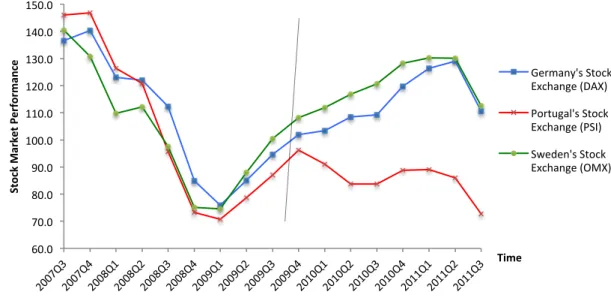
Furthermore, the European countries that were heavily indebted in early 2010 saw another massive decline and increased volatility in the stock prices when the debt crisis took off. Countries that managed a more stable debt saw a milder decline in the stock prices or not even notable movements in stock prices at all (Samiei, 2012). Figure (2) plots Portugal’s, Germany’s and Sweden’s most traded domestic stock index performance over the time period 2007:Q3 - 2011:Q3. One can clearly observe that the stock markets reacted in a similar way for all three stock indexes during the financial crisis; however, when the debt crisis started in 2010 the stock indexes performance is more diverse (Eurostat, 2012). The dashed line in Figure (2) indicates the approximate period where the debt crisis took its start.
Figure 2 Stock Market Performance (2007:Q3-2011:Q3)
Drawn from Figure (2), one can see that the Portuguese stock index (PSI) reacted more dramatically than the German stock index (DAX) and the Swedish stock index (OMX) to the debt crisis in Europe. However, it is also notable that the German stock market index saw a small ease in the growth rate as the crisis started, while the Swedish stock market performance was more stable (Eurostat, 2012). Moreover, the fact that the Portuguese stock index recovered slightly in 2011 could possibly be due to the bailout packages that were given to Portugal (Joao, 2012).
Nevertheless, the European stock markets witnessed their most volatile period in 2011 since the financial crisis in 2008. European banks feared another credit crisis, which forced them to turn to the European Central Bank (ECB) for support and advice. During 2011 it was agreed upon to give the ECB more funds to address the crisis in Europe to ease the position of other central banks as well as the stock market pressure. Moreover, as the debt crisis remains throughout Europe, the stock market continues to drop and the debt levels seem to rise (The Economist, 2011).
As illustrated it should be emphasised that not all of the European countries face similar trends in either their domestic stock market performance or in their debt level trends (Eurostat, 2012). 60.0 70.0 80.0 90.0 100.0 110.0 120.0 130.0 140.0 150.0 St oc k Ma rke t P er fo rm an ce Time Germany's Stock Exchange (DAX) Portugal's Stock Exchange (PSI) Sweden's Stock Exchange (OMX)
4 Theoretical Framework
This section will provide theory that could support the idea that government debt changes could influence stock market performance. The first subsection (4.1 Efficient Market Hypothesis) will provide evidence that support the idea by the means of the EMH and the second subsection (4.2 Budget Deficits, High Government Debt Levels, and Standard Security Evaluation Model) will give the reader insights of how debt could affect the economy and therefore also the stock market performance.
4.1
Efficient Market Hypothesis
There are many theories that aim to explain stock market movements, but they are subjective. This means that there are no objective laws that govern the financial behaviour of stocks; however, there are several ideas that attempt to explain the movements and one of the ideas is the EMH. According to Fama (1969) an efficient market is defined as the following:
‘In general terms, the ideal is a market in which prices provide accurate signals for resource allocation: that is, a market in which firms can make production-investment decisions, and investors can choose among the securities that represent ownership of firms' activities under the assumption that security prices
at any time "fully reflect" all available information. A market in which prices always "fully reflect,” available information is called "efficient."’
(Fama, 1969, p. 383) The EMH is a theory of that asset prices fully incorporate and reflect all relevant information immediately into its prices. Thus, the market price of an asset is an unbiased estimate of its true value. Under this theory, the stock prices are always characterized by their true value, meaning that assets are traded at their fair value and that it is impossible for investors to outperform the overall market. Assets cannot be purchased either through undervalued or inflated prices. According to McDowell et al. (2009) the stock prices do not only depend on the future earnings of companies but also on how investors estimate them. Moreover, investors are concerned about current earnings, the prospects of industries, the economic health of an economy and a hand full of other factors (MacDowell et al. 2009).
The EMH can be categorized into three different versions where the information reflected differs.
• The weak form of EMH states that current asset price fully reflect all the past prices of the asset. This makes it impossible to find an undervalued asset by using technical analysis that only reflects past prices of the asset.
• The semi-strong form of EMH states that prices efficiently adjust to not only past prices but also to all public available information. Publicly available information refers to new reports, financial announcements, stock splits etc. to paraphrase, this means that corporations financial statements or announcements cannot yield any valuable information about under or overvalued asset prices.
• The third category is called strong form of EMH and states that all information is reflected by the assets prices both private and public. It does not matter if investors or a company’s management have monopolistic access to inside information that could be relevant for the price of the asset since its price already reflect this material (Hagin, 1979).
By concluding, it can be stated that if variables are relevant to affect stock prices they do so without any delay depending on if the stock market is efficient or not (Fama, 1969). Hence, in case of an efficient market, if government debt levels are relevant to affect the stock market performance they do so, without any delay.
4.2
Budget Deficits, High Government Debt Levels, and
Standard Security Evaluation Model
As mentioned earlier, government debt is a term used for the accumulated past borrowing of a country. According to studies conducted by Zimmerman (1997), budget deficit appears either because
‘tax revenues fail to keep up with government spending or because tax cuts outpace cuts in government
spending’
(Zimmerman, 1997, p.65) In other words when a country cannot balance its fiscal budget and is therefor running a deficit.
However, in contrast to this stands the assumption that if a government is receiving more than it spends it is running a surplus. The budget can be illustrated as following expression: (T - G), whereas the T stands for the state’s taxation income and the G for the government spending (unemployment benefits, health care etc.). Thus, when a sovereign state is running a budget deficit it is adding up to government debt (Mankiw, 2003). It is recognized that in order to obtain sustainable economic growth in a country, a stable sound macroeconomic framework is needed. In such a framework fiscal policy plays a crucial role (Fischer & Easterly, 1990). Since borrowing finances deficits, debt will increase continuously if the state’s deficit endures over a long period, meaning that the debt will increase along with the financing of the deficits. This raises questions concerning debt sustainability and the impact on the economy of high debt levels (Macdowell et al. 2009).
High debt levels raise investors’ concerns about default. As outlined earlier, a government defaults when it cannot pay interest or principal on scheduled time. If investors fear that a government is facing higher default risk they demand higher returns or choose to allocate their investment somewhere else. This could lead to unaffordable interest rates for governments and financial market losses. If the government cannot access the financial market, it would need to use radical fiscal policies to obtain funds. Such fiscal policies could be harmful for the economic activity within the country and could eventually lead to a government debt crisis. Depending on the level of external and internal debt, such crisis could spread to foreign holds and cause crisis abroad, but only if large funds are invested in the indebted country. However, deficits may also increase the dependence on foreign lenders, which might not have the best interest for the country (Nelson, 2012).
Moreover, high debt levels can also make a country more vulnerable to crises. When a crisis hits, the government must access funds to address the crisis and if the debt level already is high, it is costly or impossible to finance the crisis by issuing more debt. In that case the country must find other ways to handle the crisis e.g. through international support or via other policy tools (Nelson, 2012).
Studies conducted by Rogoff and Reinhard (2010) find that the correlation between real GDP and debt levels differ for advanced and emerging economies. They also indicate that for a moderate level of debt-to-GDP ratio there is a weak relationship to real growth rates. However, Rogoff and Reinhard (2010) argue that indebtedness can become a threat to economic growth in the long run and the stability of a country as the debt-to-GDP ratio reaches higher levels. The researchers find that the advanced economies’ median growths are generally one percentage lower and average growth rates are several percentages lower when a government faces a debt-to-GDP ratio over 90%. Moreover, when emerging markets external debt-to-GDP ratios extend to 60%, growth rates decline by about 2% annually. Finally, as the debt burden of a country is carried forward to the next generation the government debt-to-GDP ratio depends on the new
work force. If the new generation consists of fewer labourers than the previous one the debt becomes harder to repay, i.e. they are left with a higher debt burden per capita (Nelson, 2012).
A simple security-pricing model can be helpful in explaining how the fiscal policies and a government’s finance decisions can be reflected by stock prices (Darrat, 1981). Stock prices can be calculated according to the following Equation (1).
Equation (1):
𝑃𝑉
!=
!!!
(!!!!!!!)! !
!!!
,
where 𝑃𝑉! stands for the current price of a stock and 𝐸!! symbolizes the expected earnings at time t. The 𝑖! is reflecting the risk free interest rate at time t and the 𝑟! is the
risk premium at time t.
As explained previously, MacDowell et al. (2009) argue that the expected earnings of an asset depends upon the future earnings and investor estimations, thus depending on what factors that investors are considering while investing, they affect the stock prices. MacDowell et al. (2009), state that an economy’s health is an important factor, which could influence the stock prices. In Equation (1) the estimations of the economy’s prospects and health could be included in the expected earning variable. When predictions favour the growth of an economy, the stock market reflects this growth trajectory and the stock prices would be bid up due to the expectation that future earnings will rise (Foresti, 2006).
Moreover, there are numerous factors that could be reflected in the expected earnings variable at time t that have connections to a country’s government debt level. Several researchers argue that deficits and large debt levels affect growth, investments and aggregate demand (Feldstein, 1982; Rogoff & Reinhardt, 2010; Mankiw, 2003). Investments and demand are important determinants of stock market performance since they affect a country’s economic situation. Thus, if deficits and debt levels are growing significantly then this will affect the stock market performance through the expected earnings variable (Mankiw, 2003). Moreover, Reinhardt and Rogoff (2010) argue that a high enough government debt level will cause the GDP growth to decline, which in return affects the stock market performance since it is related to an economy’s health. An economy must generate necessary revenue to afford investments that can strengthen the economy in the long run. Williams (2012) argues that countries need to generate the revenue in a transparent and equitable manner. This indicates that how a country chooses to finance its budget matters for the economy’s prospects. The variable representing expected earnings at time t in the Equation (1) could once again possibly reflect the economy’s budget decision. However, the risk premium variable would then also be affected by these variables since fiscal policies can affect the state of an economy and reflect domestic market risk (Williams, 2012). Furthermore, according to Mankiw (2003), fiscal policies also exert an influence on the risk free interest rate. When a government is running a deficit, thus increasing its debt level, the market for loanable fund will decrease causing higher interest rates and vice versa, as the government is running a surplus, the market for loanable funds will increase causing lower interest rates (Mankiw, 2003). To summarize, fiscal policies and high government debt levels could affect all the variables in Equation (1). The two theories that are provided in this section support the idea of that government debt changes could possibly affect stock prices. However, in the following section (5. Empirical Research) where the relationship between stock market performance and government debt changes will empirically be investigated, the EMH will be considered. The fact that the EMH simultaneously investigates whether government debt level changes are relevant to affect the stock market performance and
5
Empirical Research
The following subsection (5.1 Data, Variables and Descriptive Statistics) explains which variables that are used as indicators of government debt changes and stock market performance in the two empirical tests for each country. It also explains which variables that are chosen as control variables for the Ordinary Least Square regression and end with some comments on the descriptive statistics table that can be found in Table (1). To explore a possible relationship between stock prices and government debt, an Ordinary Least Square regression with time series data have been conducted for three different countries that face diverse general government debt levels as percentage of GDP over a given time period. However, since the study aims to answer whether changes in debt levels precede changes in the stock market, a causality test developed by Granger is conducted for all three countries. The results can be found in the second subsection (5.2 Empirics).
5.1
Data, Variables and Descriptive Statistics
All data series are compiled from Eurostat database (2012) over the time period 2000:Q2 - 2011:Q2. A quarterly frequency is used since it is most applicable given the need to observe debt level changes. As mentioned in previous section, the countries that are chosen for this empirical analysis are respectively: Germany, Portugal and Sweden. The countries selected are EU members that face different debt level trends for the chosen period.
• Germany’s government debt level faced an upward trend from under 60% of GDP in the beginning of 2000 to a debt level slightly under 90% of GDP in 2011 • Portugal faced a sharper increase in its government debt level over the chosen
period starting at 50% of GDP in 2000 up to a debt level over 100% of GDP in 2011.
• Sweden faced a decreasing debt level over the same period. In 2000 Sweden faced a debt level of 60% of GDP decreasing to only 40% of GDP in 2011 (Eurostat, 2012).
Moreover, a commonly used expression for a country’s debt is as a percentage of GDP. The three countries differ in economic size and therefore can manage different debt levels. The gross domestic product indicates the size of the economy and by expressing the debt as a percentage of the GDP one can use this to determine a country’s relative debt burden and changes (Nelson, 2012).
Moreover, the debt levels can be reported in several different ways. The two most common ones are the central government debt only or the total government debt (general government debt) including all the levels of government (e.g. central/federal, province/state, local) (Nelson, 2012). This empirical analysis measures the general debt level as a percentage of GDP.
Furthermore, a stock index indicates the performance of a number of stocks as a group. There are several stock indexes on different markets and most countries have their own stock index to measure the average performance of the country’s stock market (Gough, 2011). The most traded stock index within each domestic market has been chosen as an indicator of the stock market performance in this empirical research. These stock market indexes have been mentioned previously in this thesis, however, for clarification they are described further. Germany’s most traded stock market index is the Deutscher Aktien Index (DAX), and it is a total return index for 30 companies traded on the Frankfurt Stock Exchange (Bloomberg, a, N/d). Portugal’s most traded stock market index is the Portuguese Stock Index (PSI) and contains 20 stock listed companies on the Lisbon Stock Exchange (Bloomberg, b, N/d). To measure Sweden’s stock market
performance the OMX Stockholm 30 (OMX) will be used. The index is computed of 30 stock listed companies and is traded on the Stockholm Stock Exchange (Bloomberg, c, N/d).
5.1.1 Control Variables
The variables GDP, unemployment, interest rate and each country’s lagged stock index have been chosen as control variables for each country’s Ordinary Least Square regression. As outlined in the literature review, these variables were significant in pervious research and therefore chosen be included in the regression.
The GDP variable is measured at market price and is both adapted seasonally and by working days. Interest rate is the three-month interest rate at the money market. It has the same values for all EMU members, thus values for Portugal and Germany are the same. The unemployment rate is measured to be the quarterly average and is seasonal adjusted. All the time series data have been transformed into growth rates as changes from previous quarter to avoid the problem of non-stationary data.
5.1.2 Descriptive Statistics
A descriptive statistics table is given in Table (1). It gives a summary of the data set that is used in this empirical analysis.
Table (1) Descriptive Statistics
Sweden DEBT% GDP DEBT% GDP(-1) DEBT% GDP(-2) DEBT% GDP(-3) GDP STOCK INX(-1) STOCK INX UNEMPL- OYMENT INTERE- STRATE Mean -1.100 -1.107 -1.007 -1.097 0.600 -0.387 -0.380 0.496 -1.087 Median -0.990 -1.078 -0.990 -1.078 0.700 1.697 1.470 0.000 1.206 Maximum 6.127 6.127 6.127 6.127 2.300 16.654 16.654 12.862 49.430 Minimum -8.880 -8.880 -8.880 -8.880 -3.900 -27.642 -27.642 -7.551 -93.322 Std. Dev. 3.614 3.656 3.637 3.631 1.106 10.057 9.942 4.631 23.244 Observation s 45 44 43 42 45 44 45 45 45 Portugal Mean 1.663 1.431 1.435 1.409 0.129 -1.197 -1.249 2.145 -2.046 Median 1.450 1.364 1.450 1.264 0.100 0.214 0.090 2.198 0.966 Maximum 11.849 9.056 9.056 9.056 2.200 13.934 13.934 15.906 25.741 Minimum -2.632 -2.632 -2.632 -2.632 -2.300 -26.802 -26.802 -9.309 -73.933 Std. Dev. 2.819 2.380 2.408 2.431 0.829 9.459 9.357 4.798 17.524 Observation s 45 44 43 42 45 44 45 45 45 Germany
Mean 0.643 0.663 N/A N/A 0.287 -0.150 0.136 -0.694 -2.046 Median 0.291 0.299 N/A N/A 0.300 1.431 1.461 -1.258 0.966 Maximum 9.447 9.447 N/A N/A 1.900 11.441 11.441 5.407 25.741 Minimum -2.558 -2.558 N/A N/A -4.000 -27.970 -27.970 -6.714 -73.933 Std. Dev. 1.934 1.952 N/A N/A 0.963 9.914 9.153 3.292 17.524 Observation
s 45 44 N/A N/A 45 44 45 45 45
If one looks at the standard deviation values that measure the spread of observations around its mean (Gujarati, 2009), one can observe that the values for each country’s stock market index is high, meaning that the stock markets are very volatile. However,
each country. If the interest rate has a high standard deviation it means that there is high variability and consequently a higher risk connected to them (Sill, 1996).
However, looking at the mean of the government debt changes as percentage of GDP for each country, which indicates the average movement of the debt level changes, one can see that the debt change for Sweden is negative while for Germany and Portugal its positive. However it is notable to point out that the Portuguese mean value is significantly higher than the German value.
The mean value for the unemployment variable of Sweden is positive, thus the unemployment level has increased on average. It is worth stressing that Portugal’s mean value for the variable is significantly higher, meaning that Portugal saw a sharper increase in its unemployment rate. In contrast to Sweden and Portugal, the mean value of the unemployment variable for Germany is negative, which indicates that the average unemployment level has decreased over the period.
Moreover, the mean value for the GDP variable for Sweden is higher than for Germany and Portugal. This indicates that Sweden on average saw a relatively higher GDP growth for the period of interest. However, Germany saw approximately twice as much average growth of GDP than Portugal.
The overall values seem to be satisfying and in line with the economic situation of these countries. However, there are large difference between some of the variables’ mean values and median values, which could indicate that there are outliers. When plotting these values, they did not seem to be abnormal and for the stock market performance extreme values are not unusual since they are very volatile and highly speculative.
5.2
Empirics
This subsection provides the reader results from the Ordinary Least Square regressions and the results from the Granger Causality test for each country set.
5.2.1 Ordinary Least Square
The Ordinary Least Square method is one of the most popular methods used in regression analysis. The regression equation is set up of a dependent part and an independent part. If an independent variable is significant, an increase in the variable, given that all other variables are constant, will lead to an increase or decrease in the dependent variable by the independent variable’s coefficient estimate (Gujarati, 2009). Equation (2) is used for each country set in Eviews, to obtain the outputs for the Ordinary Least Squares method. However, the two variables “Debt%GDP(-2)” and “Debt%GDP(-3)” are not included in the independent part in the regression for Germany since the Akaike information criterion (AIC) are lower in Germany’s output excluding these variables.
Equation (2):
𝑆𝑡𝑜𝑐𝑘 𝐼𝑛𝑑𝑒𝑥 = 𝛽!+ 𝛽! 𝐷𝑒𝑏𝑡%𝐺𝐷𝑃 + 𝛽! 𝐷𝑒𝑏𝑡%𝐺𝐷𝑃(−1) + 𝛽! 𝐷𝑒𝑏𝑡%𝐺𝐷𝑃(−2) +
𝛽! 𝐷𝑒𝑏𝑡%𝐺𝐷(−3) + 𝛽! 𝐺𝐷𝑃 + 𝛽! 𝐼𝑛𝑡𝑒𝑟𝑒𝑠𝑡 𝑟𝑎𝑡𝑒 + 𝛽! 𝑈𝑛𝑒𝑚𝑝𝑙𝑜𝑦𝑚𝑒𝑛𝑡 + 𝛽! 𝑆𝑡𝑜𝑐𝑘 𝐼𝑁𝑋(−1) + 𝜀
Table (2) presents the empirical result of Equation (2) for each country with its domestic stock market index as the dependent variable.
In the case of Germany only three variables are significant. The variable quarterly changes in debt, as a percentage of GDP is significant at a 5% level and has a positive relation to the DAX. The control variable GDP also has a positive relation to the DAX and is significant at 5% level. Another control variable, the lagged values of the DAX is also significant at a 5% level and has a positive relation to the dependent variable. All other variables seem to be insignificant.
If one looks at the regression output for Sweden, it can be seen that only three control variables are significant and none of the quarterly changes in debt as a percentage of GDP with different lags are significant. The p-values for each one of them are high and therefore the null hypothesis of being insignificant cannot be rejected. However, quarterly changes in GDP, interest rate and lagged values of OMX Stockholm index are significant at a 5% level. The GDP and lagged OMX variables have a positive relation to the dependent variable and quarterly changes in the interest rate has a negative relation to the dependent variable. The other variable quarterly change in unemployment is insignificant.
In the regression output for Portugal one can observe that three variables are significant; the first one is the quarterly debt changes as a percentage of GDP when lagged twice. It is significant at a 1% level and has a positive relation to the quarterly changes in PSI. The other two variables, quarterly changes in GDP and lagged values of the quarterly changes in the PSI are control variables and both are significant on a 10% level. They have a positive relation the dependent variable. All other variables are insignificant.
To conclude the results, only in the outputs of Germany and Portugal the quarterly debt level changes as a percentage of GDP are significant, although with different lags. Moreover, the German quarterly stock index changes are correlated with the quarterly debt level changes without any lags for the observed period while the Portuguese stock index is correlated while two lags are included in the quarterly debt changes as a percentage of GDP. The stock indexes have a positive relation to the government debt changes. However, for the case of Sweden’s stock market index it does not have a correlation with any of the quarterly debt level changes at different lags.
5.2.2 Robustness – Ordinary Least Squares Output
In order to ensure statistical efficiency, each output has been analysed using several tests. All the variables in all three outputs have been tested for the existence of a unit root.
Table (1) Ordinary Least Square Outputs Deutcher Aktien Index
Sample: 2000:Q3-2011:Q2 OMX Stockholm Index Sample: 2001:Q1-2011:Q2 Portuguese Stock Index Sample: 2001:Q1-2011:Q2
Independent Variables
Coefficient Std. Error Coefficient Std. Error Coefficient Std. Error
Constant -2.232 (1.385) -1.955 (2.270) -5.194 (2.125) GDP 3.496** (1.680) 3.708** (1.753) 3.402* (1.916) Interest rate -0.045 (0.095) -0.196** (0.085) -0.051 (0.079) Unemployment -0.113 (0.455) -0.286 (0.419) 0.222 (0.324) STOCK INX(-1) 0.346** (0.157) 0.385** (0.149) 0.350* (0.190) Debt%GDP 1.409** (0.630) -1.156 (0.446) -0.128 (0.499) Debt%GDP(-1) 0.608 (0.654) 0.076 (0.410) 0.436 (0.557)
Debt%GDP(-2) N/A N/A 0.098 (0.460) 1.716*** (0.571)
Debt%GDP(-3) N/A N/A 0.014 (0.420) 0.426 (0.631)
R2 0.443 0.468 0.503
N 44 42 42
***- Indicates significance at a 1% level ** - Indicates significance at a 5% level * - Indicates significance at a 10% level
This is done by the Augmented Dickey-Fuller test, which shows that for each variable one can reject the null hypothesis of the existence of a unit root. Moreover, each output has been tested for autocorrelation with help of the Breusch Godfrey Serial Correlation Test. In all three cases the null hypothesis of no autocorrelation cannot be rejected. Furthermore, the data in the three outputs have been tested with a Jarque-Bera Normality test to ensure that the residuals are normally distributed. In all three cases the null hypothesis of the residuals being normal cannot be rejected. The outputs for each test from Eviews can be found in the Appendix (Table 4-7).
Each R2 in the regressions outputs for the countries lies between 0.43 and 0.50 (can be seen in Table (2)). In these cases the R2s are high enough since dealing with stock prices, which are considered to be highly unpredictable.
5.2.3 Granger Causality Test
A regression analysis discussed above indicates the dependence of one variable on other independent variables and does not necessarily mean that the independent variables cause the dependent variable. In other words, a relationship proved in an Ordinary Least Square does not imply causality. If a variable is proved to Granger-cause another variable then changes is the causing variable should precede changes in the other (Gujarati, 2009). The Granger Causality test can be illustrated for each country (j) by the following Equation (3). Equation (3): 𝑆𝑡𝑜𝑐𝑘 𝑀𝑎𝑟𝑘𝑒𝑡 𝐼𝑛𝑑𝑒𝑥!!= 𝜆! ! !!! 𝑆𝑡𝑜𝑐𝑘 𝑀𝑎𝑟𝑘𝑒𝑡 𝐼𝑛𝑑𝑒𝑥!!!! + 𝛿! ! !!! 𝐺𝑜𝑣. 𝐷𝑒𝑏𝑡!!!! + 𝑢!!
The Equation (3) indicates that the current stock price index is related to its past values as well as that of the public debt changes. The hypothesis test that is used to determine if general government debt Granger-cause the stock market is stated as followed:
H0: General government debt changes do not Granger-cause the stock market
H1: General government debt changes do Granger-cause the stock market
As Equation (3) illustrates the test is examining whether the growth rates of debt as a percentage of GDP causes the growth rates of the stock market index. The procedure starts with a restricted regression where the stock market index is regressed on its past values only. From this one obtains the sum of squared residuals (RSSR). Then a second regression is computed called unrestricted regression where the lagged debt as a percentage of GDP is included thereof one obtains the unrestricted sum of squared residuals (RSSUR). The F-statistics is calculated by the following Equation (4).
Equation (4):
𝐹 = (𝑅𝑆𝑆! − 𝑅𝑆𝑆!") 𝑚 𝑅𝑆𝑆!" (𝑛 − 𝑘)
As mentioned earlier, the null hypothesis is implying that the debt as a percentage of GDP does not Granger-cause the stock market performance. The F-test follows a distribution with m and (n-k) degrees of freedom where m represents the number lags of debt as percentage of GDP and k is representing the number of parameters estimated in the unrestricted regression. The results in Table (3) are conducted with help of Eviews for each country set.
The F-statistics for Germany and Sweden cannot be rejected with 90% confidence. However, if one look at the p-values given in the Table (3), one can see that they are very small and close to 0.10. For the case of Sweden the p-value is 0.108 and for Germany it is 0.149. If one should be consistent with the outcome of the output there seems to be no Granger-causality from the debt levels of Germany and Sweden to its respectively stock market.
In contrast to Sweden and Germany, Portugal’s F-value can be rejected with 99% confidence and its p-value is 0.007. This implies that the Portuguese general government debt granger causes the Portuguese Stock Market Index. It is proved that the past values of Portugal’s general government debt contribute to the prediction of the present value of the Portuguese Stock Market as well as its past values of itself.
5.2.4 Robustness – Granger Causality Tests
Granger Causality test requires stationary data, which the data already was tested for in previous section (Augmented Dickey-Fuller results can be found in Appendix, Table 4). Moreover, the Granger-causality test is sensitive to the choice of lag length and to avoid any limitations, a Vector Auto Regression estimate is conducted for each country set to determine the optimal lag length (Gujarati, 2009). This is done with help of AIC and the optimal lag is chosen base on the lowest AIC-value (Values can be found in Table (3)). However, other lag lengths were also tested during the analysis to evaluate the differences in the output given different lag length. However, they gave similar results.
Table (2) Granger Causality Test
Country Null Hypothesis Lag Obs. P-value F-stat. Decision
Germany Debt%GDP Does Not Granger Cause DAX 1 44 0.149 2.161 Not Rejected Portugal Debt%GDP Does Not Granger Cause PSI 2 43 0.007 5.766* Reject Sweden Debt%GDP Does Not Granger Cause OMX 2 43 0.108 2.363 Not Rejected * - Indicates significance at a 1% level
6
Discussion of Empirical Results
Since the p-values for Germany and Sweden in the Granger Causality test are insignificant the results show that the quarterly debt changes as a percentage of GDP do not Granger-cause its domestic stock market changes given the lags values. However, one should keep in mind that the values are small and close to be significant at a 10% level. Since the p-values are questionably low, the outcome of the Granger-causality test is doubtful and the interpretation of these values could be ambiguous.
The Ordinary Least Square output for Sweden shows that the quarterly debt level changes, as a percentage of GDP, do not have any correlation with the quarterly stock index changes at any lag length tested. The Granger Causality test shows that the quarterly government debt changes, as a percentage of GDP, do not Granger-cause the quarterly stock market performance given consistency with the number drawn from the result in Table (2). Based on these test one cannot see a relationship between the two variables for the case of Sweden.
As aforementioned, Fama (1969) argues that if a market is efficient, its stock prices should reflect all relevant information as soon as they occur. The empirical results show that the past values of the government debt changes do not affect the stock market performance. However, the Granger Causality test requires time lags (Gujarati, 2009), and therefore the test is limited to further evaluate the relationship given the quarterly data. One can neither reject nor accept the EMH presented by Fama (1969) in regards to government debt level changes for Sweden. Controversy, the p-value from the Granger Causality test is small and close to significant at 10% level, which could give support to reject the hypothesis presented by Fama (1969) given government debt changes. If so, then the government debt changes do Granger-cause its stock market performance with two lags lengths. Moreover, Fama (1969) declares that only if variables are relevant to affect stock market prices and do so without any delay, the market is efficient. From the Ordinary Least Square method the findings that are presented do not indicate any correlation between the government debt changes and the stock market performance for Sweden. This could possibly also strengthen the idea that the EMH should be rejected with respect to government debt changes, and that the two variables have no relationship at all.
However, Bergman (2011) claims that Sweden has been running a strict fiscal budget and their main objective was to attain fiscal stability. Moreover, the fact presented in a report by the U.S Department of Commerce (2011) reveals that the Swedish State has sold out state owned assets in order to keep its debt level down during the last five years. The Swedish government is thus stressing to keep the debt level low and this policy might have affected the outputs for Sweden given the observed period. Table (1) Descriptive Statistics also confirms the decreasing debt level that Sweden faced during the period of interest, since the mean value of government debt changes variable is negative.
Similar results are found in the outputs for Germany. The Granger Causality test was conducted with one lag and the null hypothesis could not be rejected if one should be consistent with the numbers given in the output. Therefore, the evidence could be interpreted, as if the German government debt level cannot Granger-cause the domestic stock market performance given the observed period. However, since the p-value from the output is small and close to be significant at a 10% level, this could potentially support the idea of rejecting the EMH given government debt changes. As in the case of Sweden, one can neither reject nor accept the EMH presented by Fama (1969), hence the ambiguous interpretation of the small p-value.
However, the Ordinary Least Square output showed that the quarterly debt level changes are correlated with the domestic stock market performance without any lags, thus
instantaneous correlation is found. This fact could on the other hand, possibly strengthen the idea that the German stock market is an efficient market. One could possibly conclude that if one uses a smaller frequency of the data the relationship should be clearer, hence the instantaneous correlation.
In regards to Sweden and Germany it is unclear whether their stock markets are efficient, thus, whether debt level changes could possibly affect the domestic stock market immediately as it increases or decreases. However, if one should be consistent with the p-values given in the outputs, there seem to be no Granger-causality between the two variables and it is very doubtful to assume that the Swedish and the Germany stock markets are efficient without any lags given government debt changes.
In contrast to Sweden and Germany, the evidence found in the empirical results for Portugal shows that the Portuguese government debt changes Granger-cause the domestic stock market performance with two lags. This does not correspond to what Fama (1969) outlines as an efficient market. The government debt level changes seem to affect the stock market performance, i.e. its changes are relevant, but it first affects the stock market when lagged twice. The results however, correspond to what Darrat (1990a) finds in his research regarding the United States’ government debt level changes and the domestic stock market performance. Darrat (1990a) explains that government debt changes Granger-cause the stock market with two lags, and therefore Darrat (1990a), rejects the hypothesis of the stock market being an efficient market for the United States during the observed period. Furthermore, the results from the Ordinary Least Square regression for Portugal also support the idea to reject that the Portuguese stock market is an efficient market in regards to the government debt changes. The results from the Ordinary Least Square output indicate that the Portuguese government debt changes had a positive correlation with the stock market performance when lagged twice. To clarify, the stock prices do not reflect the quarterly government debt changes immediately as they increased or decreased for Portugal, thus meaning that one should not reject that the Portuguese stock market is an inefficient market. The fact that the Portuguese stock market is Granger-caused by its quarterly government changes with two lags means that the debt level changes six months earlier Granger-cause the stock market. One could possibly think that this might be due to the inefficiency of the spread of information regarding deficit reports. However, this grows concerns regarding to monitor the Portuguese debt level changes as soon as they occur, hence it will Granger-cause the domestic stock market performance six months later according to the findings. This corresponds to what Ewing (1997) found for Australia and France. Ewing’s (1997), important conclusion implied that past deficits can aid the prediction of future movements of the stock market for both countries. This could also be the case for Portugal. One should therefore not use the stock market performance as a possible indicator of Portugal’s economic conditions as suggested by Mankiw (2003). However, this could only be supported with respect to government debt instability in the case of Portugal.
The output for Portugal is the only country that gives clear results from the Granger-causality test that also are consistent with the Ordinary Least Square regression. However, Portugal has seen the largest debt increase over the period relative to the two other countries investigated (Eurostat, 2012). The descriptive statistics table computed from the data also confirms this hence the high mean value of the government debt changes. Moreover as Samiei (2012) argues, Portugal faced fiscal imbalance and struggled with their debt management during the debt crisis. One could therefore think that the aggregated debt level plays a role in the Granger-causality. As previous research outlined by Rogoff and Reinhardt (2009), that finds that when the aggregated debt, as a percentage of GDP, reached a certain level it affected the domestic GDP growth. This could possibly be the