Interest risk in Inter-bank market in
China based on VaR model
Master thesis in economics, 15 ECTS
Programme: Economics trade and policy Author: Qing Gu, 881006-T328 Tutor: Pär Sjölander
1
Acknowledgements
I want to thank my wonderful supervisor Pär Sjölander for his help, comments and patience while working with me throughout this process.
Also I want to thanks my opponent and co-examiner for suggestions and to thanks the other students attending the thesis presentation for providing me with helpful feedback
2
Abstract
Considered as the core of financial market, commercial banks rely on the interest income. The financial market in China are more and more complete since the economic reform in 1978, in this case, measuring and preventing the interest risk become very important. This paper seeks to analyse whether Value-at-Risk (VaR) model is appropriate to measure the risk in inter-bank market in China by using the overnight Shibor from 2013-01-01 to 2014-12-31. The forecasting capabilities of various VaR models are evaluated using conditional heteroscedasticity models such as GARCH, EWMA, GARCH-M, TGARCH and EGARCH (under various distributions). It concluded that the EGARCH model (under GED distribution) most accurately explains the volatility of the Shibor (Shanghai interbank offered rate). The VaR out-of-sample forecasts constitute about-10% of the return of the Shibor. If the final model is accurate, our results indicate that the inter-bank market in China is relatively stable in the analysed and forecasted period. This suggests that the Chinese commercial banks face interest risk which cannot be defined as high.
Keywords:
3
Contents
Acknowledgements...1 Abstract ...2 1 Introduction ...5 1.1 Purpose ...6 1.2 Research questions ...7 1.3 Method ...7 2 Background ...82.1 The development of commercial banks of China ...8
2.2 Interest rate liberalizing progress in China...8
2.3 The role of Shibor ...9
3 Theoretical framework ... 11
3.1 Interest rate “gap” management... 11
3.2 Duration method ... 12
3.3 VaR methods ... 12
4 Empirical framework ... 14
4.1 Parameter VaR... 14
4.2 Models measuring for conditional variance ... 14
4.3 Forecast VaR model ... 16
4.4 The residual distribution ... 16
4.5 Back-testing of VaR ... 17 4.6 Data description ... 18 4.7 Methodology ... 19 5 Diagnostic tests ... 21 5.1 Normality test ... 21 5.2 Stationary test ... 21 5.3 Autocorrelation test... 22
4
5.4 Conditional heteroscedasticity test. ... 22
6 Empirical result ... 24
6.1 Result of GARCH family models ... 24
6.2 Result of VaR... 26 6.3 Forecast VaR... 27 7 Conclusion ... 28 References ... 29 Appendix ... 32 Table 6.1.1 ... 32 Table 6.1.2 ... 33 Table 6.1.3 ... 34 Figure 6.2.1... 35 Figure 6.2.2... 35 Figure 6.2.3... 35 Figure 6.2.4... 36 Figure 6.2.5... 36
5
1 Introduction
China financial system has experienced a great growth after the reform and opening policy in 19781, since then commercial banks of China began the process of
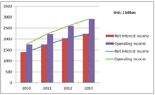
marketization. For the reason that interest income is the major income for the commercial banks in China, interest rate risk plays the most significant role in the risk management of commercial banks. It is shown in Figure 1.1 that net interest income of 16 listed commercial banks2 occupies 74.8% of their operating income in average, and its
net interest income is 1403 billion Yuan in 2010 and this number grew to 2238 billion Yuan in 2013 which increased by 59%. In this case, commercial banks‟ operation in China mainly depended on the interest income, so the series issues of interest rate management and measurement has become inevitable.
Interbank markets are of most importance in the financial system, allowing liquidity to be readily transferred from banks with a surplus to banks with a deficit (Allen et al. 2009). Interbank markets received relatively little academic attention until the financial crisis in 2007 (Alexius et al. 2014). The result of subprime mortgage crisis in 2007 was that the interbank interest rates rose sharply for all the major currencies then fell rapidly following aggressive easing by the main central banks, and then the interest rate of unsecured and secured deposits became extremely high and volatile, moreover the
1 Economic Reform and Openness Policy, implemented by Deng Xiaoping in 1978, attracted the foreign trade and investment, which brought China from centralized planning economy into market-based economy.
2 16 listed commercial banks are: Agricultural Bank of China, Bank of China, China Construction Bank, Industrial and Commercial Bank of China, China Everbright Bank, Hua Xia Bank, Nanjing Bank, China Merchants Bank, Bank of Communications, Shanghai Pudong Development Bank, Minsheng Banking Corp, Industrial Bank Co, Pin An Bank, Bank of Ningbo, China Citic Bank, Bank of Beijing.
Figure 1.1 The comparison between net interest income and operating income. Source: The date comes from the financial statements of 16 listed commercial banks.
6 default of Lehman Brothers shock the markets again (Paolo et al. 2011). On this circumstance, interbank markets have been put under the spotlight in recent years. The interbank market in China developed relatively late compared to the developed country. People‟s Bank of China3 had not established the interbank market until 1996.
China interbank market offered rate, Chibor, was formed at that time. This opened the door of market-based form of interest rates. In 1997 government released some restriction and opened the interbank bond market. In the year of 2006, Shanghai interbank market offered rate, Shibor, was established, and it has been 19 years from now since interest rate marketization process.
Benchmark rate is the basis of interest rate system of whole country, it represents the lowest interest rate, and it responses to the changes of economy. The governments in different countries want to adjust the monetary policy and interest rate policy through the benchmark rate. Different countries have different benchmark rates, United State regards federal funds rate which is interbank lending rate as their benchmark rate, United Kingdom, adopts the base rate or the official bank rate set by the Bank of England as the benchmark rate, Tokyo Interbank offered rate (Tibor) is the benchmark rate in Japan, and Germany and France use Repo rate as their bench mark rate. Another rate-London Interbank offered rate (Libor) as the benchmark rate generally used in the world. After the series policies introduced by governments to promote interest rate liberalization, many researches took attention on what rates (Chibor, Shibor, Repo rate and so on) China would select as benchmark rate. Many researchers such as Xiang and Li (2014), Fang and Hua (2009), Guang and Ke (2012) indicated that compared with the other interest rate, Shibor is more suitable to be the benchmark rate.
In this case, measure and forecast the risk through the volatility of Shibor is very important for the banks - especially the banks in China that largely rely on the interest income to manage their risk, and moreover put more attention on interest risk can keep the health of the bank system.
1.1 Purpose
In the early days, because the volatility of interest rate controlled by governments, it has been only 19 years after first step of interest liberalization. Commercial banks do less work on management of interest risk and lack of the experience of interest risk management. For the reason that the governments and the whole society pay attention on the problem of bad loan, the problem of interest risk is overlooked. Commercial banks of China always use qualitative analysis to measure the interest risk rather than quantitative analysis.
3 People‟s Bank of China is part of state council of China, which is macroeconomic regulation and control department.
7 In this paper, I apply various conditional heteroscedasticity models in order to evaluate the forecasting capabilities of various VaR (value at risk) models. Furthermore I measure the distribution pattern of interest risk, and provide a quantative measure of the interest rate risk of commercial banks of China. The purpose is to evaluate whether the VaR model is suitable to measure interest risk in China, or if commercial banks in China face too high risks in the future.
1.2 Research questions
There are three main questions in this paper:
1. Can the VaR models accurately and adequately measure the interest rate risks in China?
2. Do Chinese commercial banks face considerably large interest rate risks? 3. Forecast the future VaR.
1.3 Method
The main method of this paper is to calculate the interest risk which is one of market risks by using the parameter relative VaR model introduced by Jorion (2007). Because current volatility is the key variable in VaR model, and financial time series have the characteristic of fat tail, I choose GARCH family models from Duffile (1997) and Agnelidis et al. (2004).
8
2 Background
2.1 The development of commercial banks of China
The banking system in China began from 1949 when People‟s Bank of China (PBOC) was established. Before 1978, the Chinese financial system followed a mono-bank system where banks were part of an executive agency. After then banking reforms had been the central subject in China‟s transformation from a command economy in to a market-oriented economy (Chen et al. 2005). There were three steps of the reform of banking system. First step was from 1979 to 1988, which focused on changing the structure and function of banking system, and PBOC released its functions into four specialized state-owned banks4 (Chen et al. 2005). In that period, PBOC changed its role
to central bank, and a supervision organization. Second step was from 1988 to1994, which established three specialist policy banks5. This reform aimed to separate the policy
banks and commercial banks. The policies after 1994 can be regarded as the third step. During this period, marketization of commercial banks was gradually improved. With Central Bank law published at 1995, banking legislation was then in accord with the provisions of the Basel Committee on Banking Supervision (Chen et al. 2005). Chen et al. (2005) also point out that the separation between policy banks and commercial banks was far from complete commercial banks system of China that commercial banks had to followed policy from PBOC such as lending to the local government regardless of return.
2.2 Interest rate liberalizing progress in China
China has already made substantial progress in liberalizing its financial markets, and its interest rates in particular (Tarhan et al., 2009). The idea of interest marketization was proposed in 1993, but no progress had been made until 1995. In the year of 1996, interbank market was built and China interbank offered rate (Chibor) was opened. In the following year, government established interbank bond market, and liberalized interbank repo rate. In 2000, governments liberalized foreign lending rates, and in the year of 2004, ceiling on all lending rates has been removed. In the year of 2006, because of the subtle influence of Chibor to the financial market, the government opened the Shanghai interbank market and hoped Shanghai interbank offered rate (Shibor) can be the benchmark interest. The pricing mechanism of Shibor6 which is similar to the Libor, can
4 Agriculture Bank of China, Industrial and Commercial Bank of China
5 China Development Bank, Export-Import Bank of China, Agricultural Development Bank of China.
6 Shibor formed by quote price of 18 banks, which contains 5 state owned commercial banks and 8 joint-equity commercial banks, 2 city commercial banks, 2 foreign commercial banks and 1 policy commercial bank. The price of Shibor is based on the quote price of these 18 banks every trading day, excluding 2 highest price and 2 lowest prices and then calculate the mathematic average of the rest 14 price.
9 help the internationalization progress of financial market in China, and develop the interest rate liberalization.
The liberalizing of interest rate was largely developed the banking system. Liberalizing the deposit rate allows banks an additional channel to compete for deposits, and therefore funds their lending operations (Tarhan et al., 2009). After the year 2007, the trading volume in interbank market grew sharply that interbank market trading volume of overnight interbank offered rate7 was 8030.5 billion Yuan in the year 2007, and this
number in 2014 reached 29498.3 billion Yuan which was more than 3 times to the number in 20078.
2.3 The role of Shibor
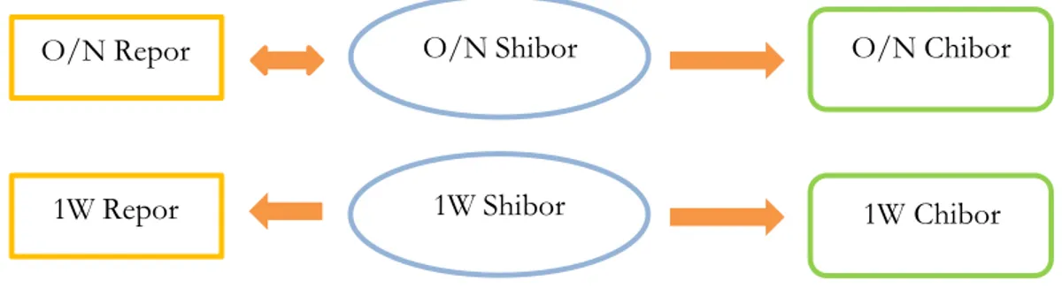
Benchmark interest plays a leading role in the interest rate system, which will not only influence the monetary policy, but also is the basis pricing elements in derivative products in financial market (Fang and Hua, 2009). It has been 9 years since Shibor was introduced by government for the first time. So many researchers in China pointed out that Shibor can be the benchmark interest in their study (Fang and Hua, 2009, Shi and Gao 2012, Peng and lu, 2010, Xiang and Li, 2014). However, there was a great debate in the literature on if Shibor can take the role of benchmark interest after 2007. The major topic of the debate was which rate (interbank offered rate or interbank repo rate) could be the benchmark rate in China. Figure 2.1 shows that the relationship of Shibor, Chibor and Repor that overnight Shibor and overnight Repor is influenced by each other, and change in overnight Shibor influenced the overnight Chibor, and overnight Chibor will not be influenced by overnight Repor. And 1 week Shibor will influence the both 1 week Repor and 1 week Chibor, and 1 week Repor independent of each other (Fang and Hua,
2009, Xiang and Li, 2014). Xiang and Li (2014) also pointed that the price of Shibor reflects the liquidity of financial market and quoted by 18 commercial banks, which are
7 There are 8 types of interbank offered rate that are overnight, 1week , 2weeks , 1month, 3 month, 6 month, 9 month, and 1 year interbank offered rate. Banks preferred the high speed of capital flow, so the overnight trading volume occupied 80% of the whole interbank market.
8 Data sources: http://www.pbc.gov.cn/publish/english/963/index.html.
O/N Repor O/N Shibor O/N Chibor
1W Repor 1W Chibor
Figure 2.1 the relationship between Repor, Shibor and Chibor.
10 high level credit rating banks that consist of state owned commercial banks, joint-equity commercial banks, city banks and foreign commercial banks. PBOC (People‟s Bank of China) signed 1670 billion Swaps, based on Shibor in 2008. So Shibor gradually influenced the price of financial products, and other interest rates.
11
3 Theoretical framework
Interest risk is one of the relative market risks, which is measured by a benchmark interest rate index (Jorion, 2007). The recent growth of interest risk management industry can be traced back to 1970s, due to the increased volatility of financial markets (Jorion, 2007). Controlled by the governments, the volatility of interest rate was relatively stable before 1970s. Since then as the progress of interest rate liberalization, many researchers pay attention to the interest rate risk management. Interest rate risk plays a role whenever agents are choosing between assets of different maturities, and poses an important problem for banks that take in short-term funds and financial long-term investment (Martin Hellwig, 1993). Martin Hellwig (1993) also points out that interest rate risk is insufficiently diversified.
Regulator has responded to increasing financial disasters that required banks and other institutions to carry enough capital to provide a buffer against unexpected losses (Jorion, 2007). The landmark Basel Capital Accord of 1988 was the first step to banks risk measurement, but it was only against credit risk, not concerned about other financial risks such as market risk, liquidity risk and operational risk. This agreement then was modified and amended to includ the market risks-interest risk in 1996. The Basel Ⅱ Accord was finalized in 2004 and implemented in 2006, which minimized the capital requirements with the regulation for at least 8% of capital in risk-weighted assets, expanded role for bank regulators, and emphasized market discipline which helped the banks to enhance their business safety and encouraged banks to publish information about their exposure risks.
3.1 Interest rate “gap” management
Mark and Chiristiopher (1984) invented a model to measure the bank interest rate sensitivity and they found that cross-sectional variation in the interest rate sensitivity measure is significantly related to the maturity mismatch of the bank assets and liabilities. In the year of 1985, Brewer introduced the interest “gap” management in which the interest income is less than interest expense, to unexpected changes in market interest rates. Banks have recognized the importance of gap management in reducing interest rate risk, achieving acceptable bank performance, and controlling size of gaps is an important function of bank funds management, and he found that the size of the gap has a major impact on the volatility (Brewer, 1985). But interest “gap” management only concerns the value in the balance sheets and ignore the change of value over time, so researchers measured many other methods and regarded interest “gap” management basic assistant method.
12
3.2 Duration method
Macaulay (1938)9 first introduced duration method to deal with the relationship between
the fixed income portfolio and the interest rate in order to measure the sensitivity of risk value of portfolio to interest rate volatility. Regardless restrictions in Macaulay duration method, researchers improved the duration method in the following years. Brewer (1985) compared different methods of interest “gap” management to found out that duration gap model is more efficient than other gap models. The difference between duration analysis and modified duration analysis is that the duration of a financial instrument is the weighted average matured of the instrument‟s total cash flow in present value terms, and modified duration can be viewed as an elasticity that estimates the percentage change in the value of an instrument for each percentage point change in market interest rates (Houpt and Embersit, 1991). Gloria (2004) pointed out that the current research on duration models offer of a succession of new models that generally use the traditional model as the only benchmark, and he tested if there are significant differences between the models. He gives the suggestion that it will get a better result when risk factors are less than three.
3.3 VaR methods
Jorion (2007) gave the definition of VaR: VaR summarized the worst loss over a target horizon that will not be exceeded with a given level of confidence. VaR method can be traced back to Markowitz‟s (1952) and in 1993, the report of G-3010 “Derivatives:
Practices and principles” first access financial risks with VaR. J.P Morgan11 introducing
RiskMetrics which is a new risk management system to calculate market risks. Basel Commission allowed banks to use VaR method to calculate the risk in 1994. The potential for gains and losses can attribute to two sources, one is exposures and the other is the movements in the risk factors (Jorion, 2007). There are many approaches of VaR to measure the market index risk, and each of them has their advantage and disadvantages.
1. Historical simulation
Historical simulation requires relatively few assumptions about the statistical distributions of the underlying market factors (Thomas and Neil, 2000). Historical simulation only needs the hypothesis that the distribution of future return is similar to the distribution of return in target horizon. If history tends to repeat, through the historical simulation, the
9 http://econpapers.repec.org/bookchap/nbrnberbk/maca38-1.htm.
10 G-30: an organization consist of top banks, financiers, and institutes from leading industrial nations. 11 https://www.jpmorgan.com/pages/jpmorgan.
13 distribution of future return can be created. Historical simulation is easy to implement and understand, but its result relies on the quality of sample in the target horizon.
2. Monte Carlo simulation
The Monte Carlo simulation can estimate VaR accurately, given enough computing resources, by Monte Carlo simulation, assuming of course that one knows the “correct” behaviour of the underlying prices and has accurate derivative-pricing models (Duffie and Pan, 1997). But if choose the wrong model, Monte Carlo simulation will fail to forecast the distribution of return, in other words, Monte Carlo simulation will have a high model risk.
3. Variance-covariance approach
The variance-covariance approach is based on the assumption that the underlying market factors have a multivariate Normal distribution (Thomas and Neil, 1996). Once the distribution of possible portfolio profits and losses has been obtained, standard mathematical properties of the normal distribution are used to determine the loss that will be equalled or exceeded X% of the time (Thomas and Neil, 1996).
The key element to VaR models is the estimation of current volatility for each underlying market (Duffie, 1997). Duffie (1997) concentrate on market risks by using VaR method, who pointed out that stochastic volatility of time series data with the properties of persistence which means that relatively high recent volatility implies relatively high forecast of volatility in the near future. Many researchers such as Orhan and Köksal (2012), Hartz et al. (2006), Anglidis et al. (2004) accurate the VaR based on GARCH family models with different distributions. Vendataraman (1997) used mixture of normal distributions, which is fat tailed and able to capture the extreme events compared to the “classical” approaches more easily. Anglidis et al. (2004) suggested that in the VaR framework the leptokurtic distributions and especially the Student‟s-t distribution with the EGARCH model is more accurate to forecast in the VaR estimation in the majority of the markets. Li and Ma (2007) used VaR method to estimate the daily Chibor, and found that VaR calculated by Student‟s-t distribution is larger than normal distribution and GED distribution. Student‟s-t distribution is not suited for China interbank market, because the GED distribution is a better method of the volatility of daily Chibor. Li (2009) calculated the VaR of Shibor from 2006 to 2007 and found out that there will be a good result under GED distribution, and that VaR method is inaccurate to measure the “right tail” of Shibor for the high volatility in the financial market at that time.
14
4 Empirical framework
4.1 Parameter VaR
Value-at-Risk (Var) is the maximum loss of an asset or asset portfolio cover a target horizon and for a given confidence level (Jorion, 2007), which is an estimation of the tails of empirical distribution (Timotheos, et al., 2004). VaR can be expressed in the function that:
( ) ( ) (1) is the loss of an asset or asset portfolio in a target period, is the confidence level and is the significant level.
For a signal asset, if the return is normally distributed, VaR can be calculated as:
( ) (2) is the quantile under X% confidence level.
Normal distribution is too simple to explain the fat tail and heteroscedasticity, but this approach is widely used because VaR is simple to calculate.
4.2 Models measuring for conditional variance
A key to measuring VaR is obtaining an estimate of the current volatility for each underlying market (Duffle and Pan, 1997). So three GARCH models that GARCH, EGARCH, TGARCH are used in this thesis to measure .
1. GARCH model
Engle (1982) introduced ARCH (q) model to estimate the volatility of financial time series data. Bollerslev (1986) proposed a generalization of the ARCH (q) model to GARCH (p q) model, the conditional variance model of GARCH (p q) model is given by:
∑ ∑ (3)
Where , and is covariance stationary if ∑ ∑ .
One special case of GARCH (1 1) model is EWMA (Exponentially Weighted Moving Average) model that ( ) ,in EWMA model parameter
15 determines the “decay” that high means slow decay. RiskMetrics only use one decay factor for all series that for daily data and for monthly data.
The GARCH (p q) model has some advantages that can successfully capture the thick tailed returns and volatility clustering of financial time series (Timotheos et al., 2004), but it cannot capture the asymmetry in volatility and cannot explain the leverage effect in time series.
The theory of GARCH in mean suggested that the mean return would be related to the variance of return. The GARCH (1 1)-in-mean is characterized by:
(4) (5)
(6) The effect that higher perceived variability of has on the level of is captured by the parameter .
2. EGARCH model
Nelson (1991) introduced the EGARCH (exponential GARCH) model, no restriction need to be imposed on the model estimation, since the logarithmic transformation ensures that the forecasts of the variance are non-negative (Timotheos et al., 2004). So the variance equation of EGARCH (p q) model can be expressed as:
( ) ∑ . | |
/ ∑ ( )
(7)
The parameters allow for the asymmetric effect and it captures the leverage effect of volatility. If , the model is symmetric. If , the good news generate less volatility than bad news. If , the good news generate more volatility than bad news.
3. TGARCH model
TGARCH (threshold GARCH) model is widely used to explain the leverage effect of time series. Zakaran (1990) express the variance equation model as:
∑ ∑ (8)
If and then otherwise , If , the leverage effect exist in time series. The good news have an impact of and bad news have an impact of . If , there is a leverage effect and if the impact of news is asymmetric.
16
4.3 Forecast VaR model
For Angelidis et al. (2004), one –step- ahead VaR forecast function can be written as: | ( ) ̂ | (9)
is the quantile under confidence level12 95%, 99% of the assumed distribution,
| is the forecast conditional standard deviation at time t+1 given the information at
time t.
For the one-step-ahead conditional variance forecast, GARCH (p q) model |
equals:
̂ | ∑ ∑ (10)
For the one-step-ahead conditional variance forecast, EGARCH (p q) model |
equals: ( ̂ | ) ∑ . | | / ∑ ( ) (11)
For the one-step-ahead conditional variance forecast, TGARCH (p q) model
equals:
̂ ∑ ∑ (12)
4.4 The residual distribution
The unpredictable component can be express as (Timotheos et al., 2004):
(13)
Where is assumed to be normal distributed based on Engle (1982).
But Bollerslev (1986) proposed the standardized t-distribution with degrees of freedom with a density given by:
( ) . / . /√ ( )( ) (14)
17 Where ( ) ∫ is the gamma function and is the parameter which described the thickness of the distribution tails.
Nelson (1991) introduced another fat-tail distribution GED (generalized error distribution) with the density equal to:
( ) ( | . | )
/ ( ) (15)
Where is the tail-thickness parameter and
[ ( )
( )]
(16)
when , GED is standard normally distributed. when , GED is fat-tail distributed, when , GED is thinner-tail distributed.
4.5 Back-testing of VaR
Value-at-Risk (VaR) is the maximum loss of an asset cover a target horizon. If the loss of a day exceed the VaR, which means the VaR model fail to estimate the loss of the asset. So Kupiec (1995) introduced the back-testing to test if VaR model is efficient. The hypothesis of beck-testing is:
Where is significant level, is confidence level, m is observed number of days, n is failure of days, and is failure ratio.
To construction a statistics that:
,( ) - * 0 . /1 ( ) + (17)
Where N is the day of fail, T is the number of sample, p is the probability.
LR follow the ( ), when LR is significant larger than the quantile under certain confidence level, then reject the null hypothesis otherwise accept the null hypothesis. Through the observed number of days-m, I can get the refuse interval and the accept interval. So the key factor to test the efficiency of VaR is the failure day-n.
18
4.6 Data description
In this thesis, I choose the data of overnight Shibor in periods from 1st January 2013 to
31th December of 2014 with the sample size 501 days. Let (
)
denote the continuously compound rate of return from time t-1 to t.
In the figure 4.5.1, there is a rapid growth of interbank market trading volume since the middle of 2006 when Shibor was established. It is shown in the yearly trading volume that the trading volume was steady around 270 billion Yuan since 2011, although there is a jumped in 2012.
Figure 4.5.1 Overnight Interbank lending trading volume from 2001 to 2014 and Interbank lending trading volume from 200201 to 201411. Data source: Statistics and Analysis Department of The people's bank of China
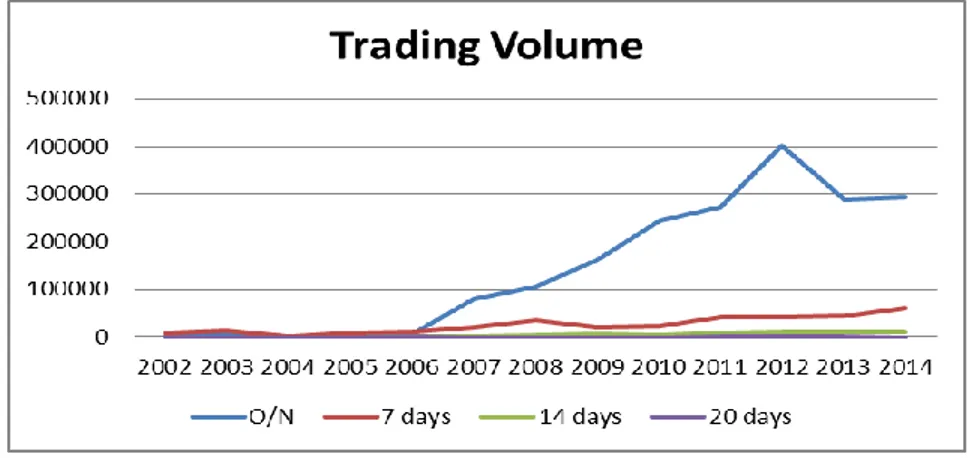
Figure 4.5.2 overnight/ 7days/ 14days/ 20days interbank lending trading volume from 2002 to 2014. Data source: Statistics and Analysis Department of The people's bank of China
19 It is shown in Figure 4.5.2 that the overnight interbank trading volume is much larger than the other types such as 7 days trading volume, 14 days trading volume and 20 days trading volume. There is a huge increase since 2006 in overnight trading volume, and it is obvious from Figure 4.5.2 that overnight trading volume occupied the interbank market. I choose the data from 2013-01-01 to 2014-12-31, for this target horizon avoid the finance crisis of 2007, which will increase the unexpected loss in the “tail”, so the VaR in this period will be more reliable. Commercial banks in China rely on the interest income, and as the different of monetary policy, Shibor may be shocked and with the different fluctuation compared to the last period, for example, if governments what to recover the economy, PBOC will adopt the policy of reduction of interest13, so Shibor will reduce for
this decision. In this case, short-term one day VaR will be more accurate than the long-term one day VaR. For the other reason, it has been 9 years since Shibor was introduced in 2006, overnight trading volume has the largest trading volume in the interbank market, and has a rapid growth after 2007 and tend to be stable in recent years. The bulk of data is sourced from The People‟s Bank of China14.
4.7 Methodology
My paper is based on the model introduced by Duffie (1997) and Angelidis et al. (2004). In this paper I will use parameter method to calculate VaR. and estimate relative VaR under three distribution assumptions that normal distribution, t distribution and GED distribution.
Let ( ) as the continuously compound rate of return of Shibor from time t-1 to t.
VaR function can be written as:
( ) (18) is the quantile under confidence level15 95%, 99% of the assumed distribution,
is the conditional standard deviation at time t.
AR (1)-GARCH (1 1) specification is most frequently applied model to empirical studies (Angelidis et al. 2004, Orhan and Köksal, 2012, Mike and Philip, 2006). So I will use AR (1)-GARCH (1 1) model to measure the fluctuation of Shibor.
AR (1) as its mean equation:
(19)
13 Reduction of interest rate is the policy used by government to change the cash flow. 14 http://www.pbc.gov.cn/publish/diaochatongjisi/126/index.html.
20 I use GARCH (1 1), EWMA, GARCH (1 1)-M, EGARCH (1 1) and TGARCH (1 1) to estimate conditional variance.
For GARCH (1 1) model equals:
(20) For EWMA model equals:
( ) (21) For GARCH (1 1)-M
(22)
(23) For TGARCH (1 1) model equals:
(24)
For EGARCH (1 1) model equals: ( ) . |
|
/ ( ) (25)
In order to measure the future, I need to measure the future first. The method
introduced by Angelidis et al. (2004) that one-step-ahead conditional variance |
which means the variance in the next day based on the massage of the variance today. After determining the by using three different distribution (normal, student-t, and GED), I use the VaR model show in equation (11) to estimate the dynamic VaR, and compare it to the (the return of Shibor), I can find the failure day that VaR exceeds the real loss of that day. In the final step I will calculate the LR statistics (equation 11) to see that whether parameter VaR works to estimate the risk of Shibor, and find out which member of the GARCH family models (with which distribution) are the most suitable model using in China interbank market.
21
5 Diagnostic tests
5.1 Normality test
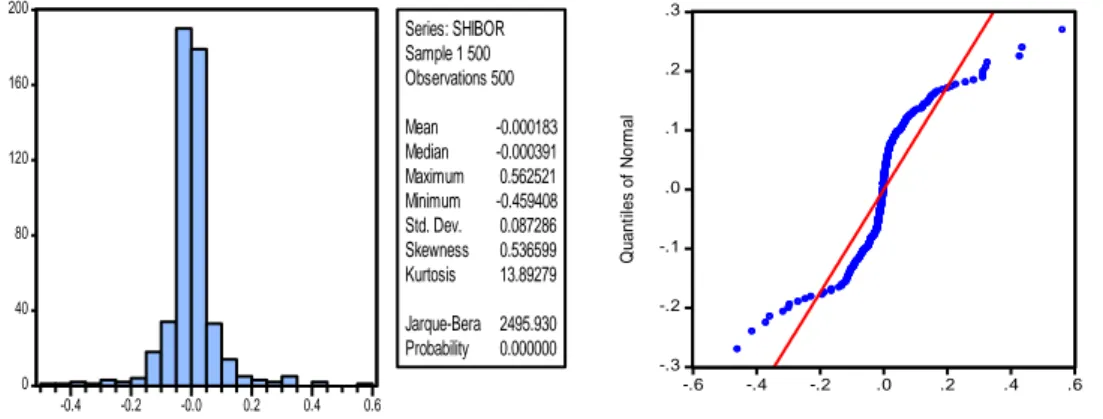
If the return is normally distributed, VaR can be simply calculated, otherwise, other tests to define the fluctuation of the data are needed. The Figure 5.1.1 shows that the mean of the return of the Shibor is -0.0001, the standard deviation is 0.087, the skewness is 0.536, and the kurtosis is 13.89, which shows the distribution can be better described as the peak and right-skewed. If the data is normally distributed, JB statistic will be smaller than the critical value of Chi-square distribution under the confidence level of 95% (5.99), but the JB statistic is 2495.930 which are much larger than the 5.99 with the probability 0, so the return of Shibor does not match the normal distribution.
From the Figure 5.2.1 shows that the line of the data does not match the line of normal distribution, but like the „S‟. So the sample of return of Shibor is not normally distributed, and with the character of peak and fat-tail.
5.2 Stationary test
I use ADF test to test the stationary of return of Shibor, from the Table 5.2.1, I can see that the result of ADF test is -18.399, and is smaller than the critical value under significance level 1%, 5% and 10% with the probability 0, so I can reject the null hypothesis. The data of return of Shibor is stationary.
Table 5.2.1 The result of ADF test. Critical Values of 1% level is -3.44, of 5% level is -2.86, of 10% level is -2.56.
t-Statistic Prob.
ADF test statistic -18.399 0.000
0 40 80 120 160 200 -0.4 -0.2 -0.0 0.2 0.4 0.6 Series: SHIBOR Sample 1 500 Observations 500 Mean -0.000183 Median -0.000391 Maximum 0.562521 Minimum -0.459408 Std. Dev. 0.087286 Skewness 0.536599 Kurtosis 13.89279 Jarque-Bera 2495.930 Probability 0.000000
Figure 5.1.1 The descriptive Statistics.
-.3 -.2 -.1 .0 .1 .2 .3 -.6 -.4 -.2 .0 .2 .4 .6 Quantiles of SHIBOR Q u a n ti le s o f N o rm a l
22
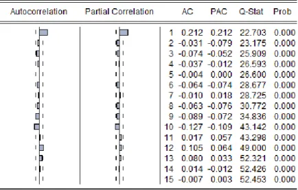
5.3 Autocorrelation test.
It shows in Figure 5.3.1 that the data has the autocorrelation problem since the AC and PAC are both different from zero. And since all the LBQ p-values are less than 5%. So I can see there is autocorrelation in the return of Shibor. In this case, I establish an AR-GARCH model that mean equation use AR model and variance model use GARCH family models to measure the conditional variance.
Because the data of return of Shibor has the problem of autocorrelation, after having comparing the AIC and SC in table 5.3.2 I can see that AIC is smallest when p=1 and q=2 and SC is smallest when p=1 and q=0, because the difference is very small. AR(1)-GARCH(1 1) is appropriate in this case.
5.4 Conditional heteroscedasticity test.
After defining the mean value model, I need to find if the model have the ARCH effect. I use ARCH-LM Test to find if the sample has the heteroscedasticity problem. It is shown in Table 5.4.1 that the ARCH-LM statistic is 68.331 with the probability equal 0,
Figure 5.3.1 Autocorrelation of return of Shibor.
23 which is smaller than 0.05 (significant level), so there is a heteroscedasticity problem in the sample. In 1982, Engle first used ARCH model to research on the variance of time series data, and Bollerslev (1986) generalized ARCH model to GARCH model.
Table5.4.1 The result of ARCH-LM test.
Heteroskedasticity Test: ARCH
F-statistic 68.331 Prob. F (1, 497) 0.000
24
6 Empirical result
The this paper I use AR(1)-GARCH(11),AR(1)-EWMA, AR(1)-GARCH(11)-M, AR(1)-EGARCH(11) and AR(1)-TGARCH(11) in three different distributions that normal distribution, Student‟s t distribution and GED distribution respectively to measure the fluctuate of Shibor. I also used AR (n)-GARCH family (1 1) to see if there can be the better result, but they cannot show the better result compare than AR (1)-GARCH family (1 1) models.
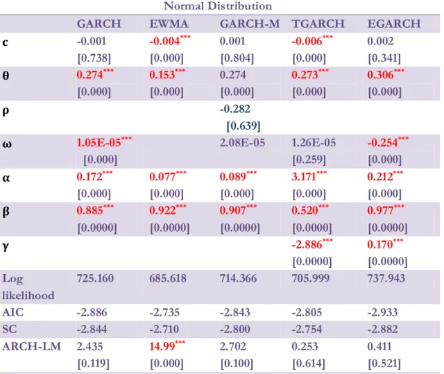
6.1 Result of GARCH family models
It is shown in Table 6.1.1 that the result of GARCH, EWMA, GARCH-M, TGARCH and EGARCH model under normal distribution. Most of the parameters are significant under 99% confidence level. And most of the models pass the ARCH-LM test except EWMA model, which mean without EWMA model the residual in other models don‟t have the problem of heteroscedasticity. So EWMA model is not suit for measure the volatility of Shibor. Although the most of the parameters in GARCH model is significant in 1% level, but the result cannot satisfied the restriction , in this case, the result of conditional variance is not stationary. Compare to the GARCH and EWMA model, GARCH-M, TGARCH and EGARCH model can explain the volatility of Shibor better. in GARCH-M, TGARCH, EGARCH models is 0.907, 0.520 and 0.977 respectively, which means that the volatility in the last period will influence much in this period, and there is a high sensitivity of interbank market with the high frequency trading. This is matching the characteristics interbank market of one day Shibor. And for is -2.886 in TGARCH model and 0.170 in EGARCH model, so it is obvious leverage effect in interbank market, which bad information will bring small fluctuation and good information will bring big fluctuation in other words the decrease (increase) of interest rate yield will lead the decrease (increase) of fluctuation of interest rate. The parameter is the risk premium coefficient shows the relationship between the return and risk, and is generally positive in financial market, which means the high risk corresponding to the high return. The in inter-bank of China is -0.282 but is insignificant.
It is shown in Table 6.1.2 that the result of GARCH, EWMA, GAECH-M, TGARCH and EGARCH model under Student‟s t distribution. Most of the coefficients are insignificant under given confidence level. But EGARCH model show a better result compare to the other model under Student‟s t distribution. It should be noted that parameter is significant under 99% confidence level in EGARCH model given the number of 0.974, which means the volatility of daily Shibor in the day before have a continuous shock on the volatility in current day. in EGARCH model is 0.181 > 0 that means the market is more sensitivity for good news than bad news. Degrees of freedom is little bigger than 2 that means the Student‟s t distribution can describes the
25 fat-tail in time series of Shibor. Although Student‟s t distribution can better describe the fat-tail, but the most of the coefficients are insignificant so Student‟s t distribution is not suit to describe the fluctuation of return of Shibor.
Table 6.1.3 shows the result of GARCH, EWMA, GARCH-M, TGARCH and EGARCH model under GED distribution. Like the result in normal distribution, the most of the coefficients are significant in GED distribution. But as the same result in GARCH and EWMA under normal distribution, GARCH model cannot satisfied the stationary and EWMA model have the ARCH-LM effect, GARCH and EWMA model cannot explain the volatility of return of Shibor in a good way. And the same result of that previous fluctuation influence much in the current fluctuation and will decay slowly. is -0.744 in TGARCH model and is 0.135 in EGARCH model which indicate that there is a leverage effects in one day Shibor, and asymmetric information on the market, under this circumstance, good news influence more than bad news. The log likelihood in GED distribution is bigger than in normal distribution and Student‟s t distribution and AIC and SC is smallest in three distributions. So GED distribution can better describe the distribution feature of one day Shibor. GED parameters are less than 2 in three models which mean GED distribution can better describe the leptokurtosis and fat-tail in return distribution of Shibor. The coefficient in GARCH-M model is negative and is significant under 1% significant level, which means the more the risk the lower the interest return, which shows the immaturity of inter-bank market in China. To sum up, compared to normal distribution and Student‟s t distribution, GED distribution can better describe the leptokurtosis and fat-tail in return distribution of one day Shibor. Compared to the GARCH and EWMA model, GARCH-M, TGARCH and EGARCH can explain the fluctuation of return of Shibor better. As showing in the result, previous shock has a significant impact on current fluctuation and will decay slowly. Different from other financial market, interbank market in China has different a leverage effect that good new influence market more than the bad news, and shows the asymmetric information on the market. Furthermore, coefficient is significant under 99% confidence level in EGARCH model under GED distribution, which shows the immaturity circumstance in inter-bank market of China. But many coefficients under Student‟s t distribution are insignificant, so Student‟s t distribution is no suits to measure the characteristics in interbank market in China, and GARCH and EWMA model cannot measure the fluctuation of interest rate return at any of the distributions (normal distribution, Student‟s t distribution and GED distribution), so I will use the GARCH-M model under GED distribution, TGARCH and EGARCH model under normal distribution and under GED distribution respectively to estimate the VaR.
26
6.2 Result of VaR
The result of VaR showing from Figure 6.2.1 to Figure 6.2.5 in 99% confidence16 level
with 3 different models that GARCH-M under GED distribution, TGARCH and EGARCH models under normal distribution and under GED distribution respectively. It is clearly shown that the maximize VaR based on TGARCH model under normal distribution and GED distribution similar to the maximize VaR based on GARCH-M model under GED distribution are much larger than the VaR based on EGARCH model under normal distribution and under GED distribution. The fluctuation of VaR based on GARCH-M model under GED distribution is far away from the fluctuation of return of one day Shibor. Fluctuation of VaR in EGARCH model under normal distribution and under GED distribution is close to the fluctuation of return of one day Shibor, moreover VaR in EGARCH model under normal distribution and under GED distribution has the smallest maximize value. All in all, compare from the Figure 6.2.1 to the Figure 6.2.5, VaR estimate based on EGARCH under GED distribution show the best result.
In order to judge the effectiveness of VaR I will use back-testing model introduced by Kupiec (1995).
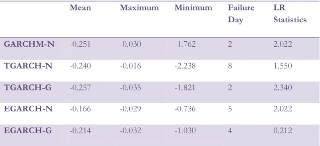
Mean Maximum Minimum Failure
Day LR Statistics GARCHM-N -0.251 -0.030 -1.762 2 2.022 TGARCH-N -0.240 -0.016 -2.238 8 1.550 TGARCH-G -0.257 -0.035 -1.821 2 2.340 EGARCH-N -0.166 -0.029 -0.736 5 2.022 EGARCH-G -0.214 -0.032 -1.030 4 0.212
Table 6.2.1 Result of VaR and Back-testing. The quantile of chi square distribution under 99% confidence level is 6.635. If LR statistics less than 6.635, It will say the model pass the Back-testing.
According to Table 6.2.1 all of the models pass the back-testing that means GARCH-M model, TGARCH model and EGARCH model under normal distribution and under GED distribution is good to predict risk in interbank market of China. More precisely, the maximum loss based on GARCH-M model under GED distribution, TGARCH
16 The quantile of normal distribution 99% confidence level is 2.326348. The quantile of GED distribution under 99% confidence level in GARCH-M model is 3.069228, in GARCH model is 3.05856, in TGARCH model is 3.066388, in EGARCH model is 3.053881.
27 model under normal distribution, TGARCH model under GED distribution are much larger than 1, which means the banks will loss more than 100% of their returns. The maximum loss based on EGARCH model is much smaller compare to the rest of the models, the maximum loss based on EGARCH under GED distribution is 100.3% and the loss under normal distribution is 73.5% of their return. Result of mean VaR in EGARCH under GED distribution is 21.4%, and under normal distribution is 16.6%. In this case, although all the models pass the Back-testing, the VaR in EGARCH model can predict the loss better than the rest of the models. And this shows the same result to the Figures. But for the GED distribution has better the characteristics of peak and fat tail of the fluctuation of Shibor. So I will use EGARCH-G model to predict the future VaR.
6.3 Forecast VaR
For my data is from 1st January 2013 to 31th December 2014, with the sample size 500,
and I will predict VaR of next 59 days to 30th March 2015. The method is to calculate
one-step-ahead conditional covariance based on Angelidis (2004). The result can be show as follows:
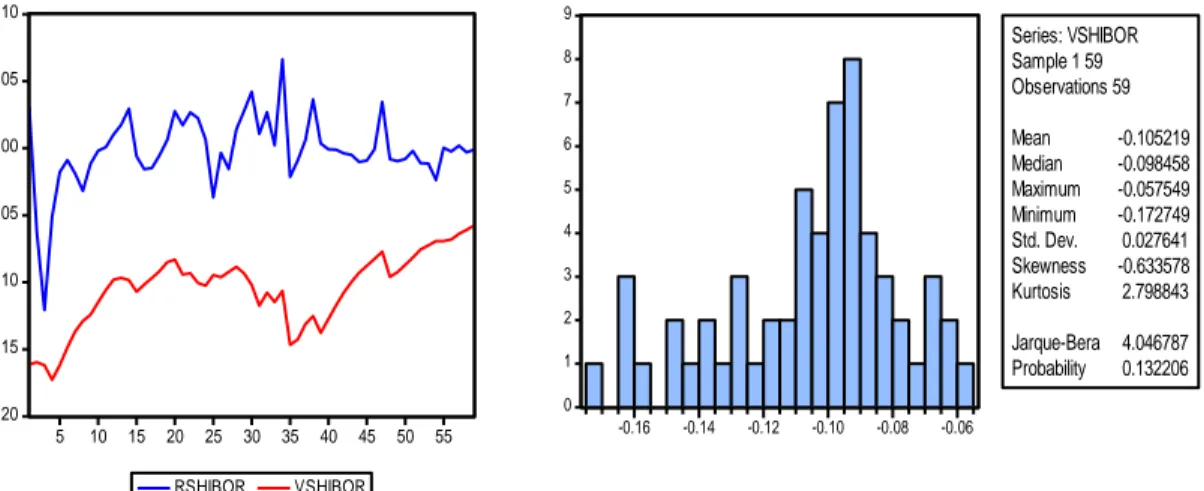
It can be seen in Figure 6.3.1 and Figure 6.3.2 that the forecast VaR can measure the risk of Shibor properly. The real loss in Figure 6.3.1 is not exceeding the VaR, and the fluctuation of VaR close to the fluctuation of return of Shibor. The maximum loss is 17.2% of the return and the average loss is 10% of the return, and the standard deviation is 0.027 which means the bank will not pay much on the prepare for the uncertain loss. So as the forecast I can say under 99% confidence level, average loss of return of Shibor will not exceed 10% in the period 1th January 2015 to 30th March 2015.
-.20 -.15 -.10 -.05 .00 .05 .10 5 10 15 20 25 30 35 40 45 50 55 RSHIBOR VSHIBOR
Figure 6.3.1 Forecast VaR. RSHIBOR is real fluctuation in return of Shibor, VSHIBOR is forecast VaR.
0 1 2 3 4 5 6 7 8 9 -0.16 -0.14 -0.12 -0.10 -0.08 -0.06 Series: VSHIBOR Sample 1 59 Observations 59 Mean -0.105219 Median -0.098458 Maximum -0.057549 Minimum -0.172749 Std. Dev. 0.027641 Skewness -0.633578 Kurtosis 2.798843 Jarque-Bera 4.046787 Probability 0.132206
28
7 Conclusion
This paper used the VaR method based on GARCH family models under normal distribution, Student‟s t distribution and GED distribution to estimate the interest risk faced by commercial banks by using the data of overnight Shibor from 2013-01-01 to 2014-12-31.
The result shows that the fluctuation of return of Shibor does not follow the normal distribution, and it has the character of peak and fat-tail. The EGARH model under GED distribution can describe the characteristics of interest rate return in appropriate way. It suggests that the historical variance of EGARCH model has a significant influence on variance right now, and the coefficient of historical term is close to one, which means the influence of historical variance is persistent and decay slowly. There is a leverage effect and asymmetric information on the inter-bank market that good news has a greater influence on fluctuation of Shibor than the bad news. Moreover, the parameter of risk premium is negative in the GARCH-M model which shows the high risk is not compensated by the high return, so the inter-bank market in China is immaturity.
By using the conditional covariance as the key factor in the VaR method, I get five different VaR series based on GARCH-M model under GED distribution, TGARCH model under normal and GED distribution individually and EGARCH model under normal and GED distribution respectively. Compare to the these five VaR series, the VaR series from EGARCH model under GED distribution and under normal distribution is close to the fluctuation of return of Shibor. From the out of sample data based on GARCH model under GED distribution, I found that the VaR method is sufficient to calculate the loss of the interest rate fluctuation from 2015-01-01 to 2015-03-31. The result indicates the interest risk faced by commercial banks cannot be defined as high.
Many researchers extend the VaR method to focus the fluctuation in the “tails” such as conditional VaR, which can describe the extreme loss in the tails (the loss larger than the loss in the confidence level), by different technologies such as Monte Carlo simulation and stress testing that can calculate the more precise VaR.
Lastly, the VaR method will loss effectiveness under extreme financial circumstance such as the financial crisis in 2007, so I suggest the VaR method will not cover a long time will help the commercial banks for their interest risk managemet.
29
References
Alexius, A., Birenstam, H., Eklund, J., 2014. The interbank market risk premium, central bank interventions, and measures of market liquidity, Journal of International Money and Finance 48 (2014) 202-217.
Allen, F., Carletti, E., Gale, D., 2009. Interbank market liquidity and central bank intervention, Journal of Monetary Economics 56 (2009) 639-652.
Angelidis, T., Benos, A., Degiannakis, S., 2004. The use of GARCH models in VaR estimation, Statistical Methodology 1 (2004) 105-128.
Brewer, E. 1985. Bank gap management and the use of financial futures. FRB Chicago Economic Perspectives, 12-12.
Bollerslev, T., 1986. Generalized autoregressive conditional heteroscedasticity, Journal of Econometrics 31 (1986) 307-327.
Chen, X., Skully, M., Brown, K., 2005. Banking efficiency in China: Application of DEA to pre- and post-deregulation eras: 1993-2000, China Economic Review 16 (2005) 229-245.
Duffle, D., Pan, J., 1997. An overview of value at risk, Journal of Derivaties, Vol. 4, No. 3, 1997, pp. 7-49.
Engle, R. F., 1982. Autoregressive conditional heterosedasticity with estimates of the variance of U.K. inflation, Econometrica 50 (1982) 987-1008.
Gloria, M. S., 2004. Duration models and IRR management: A question of dimensions?, Journal of Banking and Finance 28 (2004) 1089-1110.
Hartz, C., Mittnik, S., Paolella, M., 2006. Accurate value-at-risk forecasting based on the normal-GARCH model, Computational Statistic and Data Analysis 51 (2006) 2295-2312. Hellwig, M., 1994. Liquidity provision, banking, and the allocation of interest rate risk, European Economic Review 38 (1994) 1363-1389. North-Holland.
Houpt, J. V., Embersit, J. A., 1991. A method of evaluating interest rate risk in U.S. commercial banks, Federal Reserve Bulletin, 1991 August, 625-637.
Jorion, P., 2007. Value at risk: the mew benchmark for managing financial risk, New York: McGraw-Hill, 3 edition, ISBN: 0-07-146495-6 (inb.).
Kupiec, P. H., 1995. Techniques for verifying the accuracy of risk measurement model, The Journal of Derivatives 3 (1995) 73-84.
30 Fang, X., Huan, M., 2009. Can Shibor become the benchmark interest rate of China’s monetary market?-Empirical analysis based on Shibor data during the period of Jan. 2007-Mar.2008. Economist, 2009-01.
Li, L., 2009. The effectiveness of VaR model on Shibor, Financial Research, No.9, 2009, General No. 351.
Li, C., Ma, G., 2007. The application of VaR model in the interbank market of China. Financial Research, No. 5, 2007, General No. 323.
Macaulay, F. R., 1938. Some theoretical problems suggested by the movements of interest rates, bond yields and stock prices in the United States since 1856. NBER Books, 1938.
Mark, J. F., Christopher, M. J., 1984. The effect of interest rate changes on the common stock returns of financial institutions, The Journal Of Finance, Vol, XXXX, No.4.
Markowitz, H. M., 1952. Portfolio selection. Journal of Finance, 1952, 7(1):77-91.
Nelson, D., 1991. Conditional heteroskedasticity in asset returns: a new approach, Econometrica 59 (1991) 347-370.
Orhan, M., Köksal, B., 2012. Acomparison of GARCH models for VaR estimation, Expert System with Application 39 (2012) 3582-3592.
Paolo, A., Andrea, N., Cristina, P., 2009. The interbank market after August 2007: what has changed, and why?, Journal of money, credit and banking, Vol. 43, No.5.
Peng, H., Lu, W., 2010. Research on interbank interest in financial market of China, Management world, 11th 2010.
RiskMetrics, 1995. Technical Document, J.P. Morgan, New York, USA.
Shi, G., Gao, K., 2012, Effective test of Shibor as the benchmark interest in China, Financial science, 2/287.
Tarhan, F., Porter, N., Takats, E., 2009. Interest rate liberalization in China, IMF Working Paper, WP/09/171.
Thomas, J. L., Neil, D. P., 2000. Value at risk. Financial Analysts Journal, March/April 2000, Volume 56 issue 2.
Thomas, J. L., Neil, D. P., 1996. Risk measurement: an introduction to Value at Risk, in Finance 960906, Economics working paper archive EconWPA.
Venkataraman, S., 1997. Value at risk for a mixture of normal distributions: the use of quasi-Bayesian estimation techniques, in: Economic Perspectives, Federal Reserve Bank of Chicago, PP. 2-13.
31 Xiang, W., Li, H., 2014. The characteristics of money market benchmark rate and empirical study of shibor, Economic review, 1th 2014.
32
Appendix
Table 6.1.1The result of GARCH, EWMA, GARCH-M, TGARCH and EGARCH model under normal distribution.
Normal Distribution
GARCH EWMA GARCH-M TGARCH EGARCH
-0.001 [0.738] -0.004*** [0.000] 0.001 [0.804] -0.006*** [0.000] 0.002 [0.341] 0.274*** [0.000] 0.153*** [0.000] 0.274 [0.000] 0.273*** [0.000] 0.306*** [0.000] -0.282 [0.639] 1.05E-05*** [0.000] 2.08E-05 1.26E-05 [0.259] -0.254*** [0.000] 0.172*** [0.000] 0.077*** [0.000] 0.089*** [0.000] 3.171*** [0.000] 0.212*** [0.000] 0.885*** [0.0000] 0.922*** [0.0000] 0.907*** [0.0000] 0.520*** [0.0000] 0.977*** [0.0000] -2.886*** [0.0000] 0.170*** [0.0000] Log likelihood 725.160 685.618 714.366 705.999 737.943 AIC -2.886 -2.735 -2.843 -2.805 -2.933 SC -2.844 -2.710 -2.800 -2.754 -2.882 ARCH-LM 2.435 [0.119] 14.99*** [0.000] 2.702 [0.100] 0.253 [0.614] 0.411 [0.521] p-value within brackets. *** significant on 1% level, **significant on 5% level, * significant on 10% level.
AR(1) model defined in equation (19), GARCH(1 1) model defined in equation (20), EWMA model defined in equation (21), GARCH-M model defined in equation (23), TGARCH model defined in equation (24), EGARCH model defined in equation (25).
Restriction for GARCH (11) model: . Restriction for TGARCH (11) model:
33
Table 6.1.2 The result of GARCH, EWMA, GARCH-M, TGARCH and EGARCH model under Student‟s t distribution.
Student’s t Distribution
GARCH EWMA GARCH-M TGARCH EGARCH
-0.0006 [0.506] -0.0001 [0.835] 0.001 [0.779] -0.0003 [0.752] -0.0003 [0.700] 0.256*** [0.000] 0.253*** [0.000] 0.258*** [0.000] 0.290*** [0.000] 0.256*** [0.000] -0.003 [0.990] 0.026 [0.997] 0.028 [0.995] 0.077 [0.999] -0.346*** [0.000] 380.580 [0.997] 0.08459*** [0.000] 476.312 [0.995] 2105.494 [0.999] 0.613* [0.062] 0.643*** [0.000] 0.915*** [0.000] 0.620*** [0.000] 0.584*** [0.000] 0.974*** [0.000] -1456.073 [0.999] 0.181* [0.088] Student’s t 2.000618 2.615302 2.000562 2.000242 2.136224 Log likelihood 900.6737 883.8249 904.2780 905.2093 901.4654 AIC -3.585 -3.526 -3.596 -3.600 -3.585 SC -3.535 -3.492 -3.537 -3.540 -3.525 ARCH-LM 0.001 [0.972] 19.55*** [0.000] 0.001 [0.967] 0.000 [0.983] 0.022 [0.880] p-value within brackets. *** significant on 1% level, **significant on 5% level, * significant on 10% level.
AR(1) model defined in equation (19), GARCH(1 1) model defined in equation (20), EWMA model defined in equation (21), GARCH-M model defined in equation (23), TGARCH model defined in equation (24), EGARCH model defined in equation (25).
Restriction for GARCH (11) model: . Restriction for TGARCH (11) model:
34
Table 6.1.3 The result of GARCH, EWMA, GARCH-M, TGARCH and EGARCH model under GED distribution.
GED Distribution
GARCH EWMA GARCH-M TGARCH EGARCH
7.62E-09 [0.329] 3.18E-05 [0.884] 0.0006*** [0.001] 0.0001 [0.706] 0.0001 [0.638] 0.268*** [0.000] 0.230*** [0.000] 0.253*** [0.000] 0.270*** [0.000] 0.252*** [0.000] -0.192*** [0.001] 2.84E-05 [0.104] 2.99E-05** [0.084] 4.10E-05** [0.045] -0.314*** [0.000] 0.406*** [0.000] 0.089*** [0.000] 0.506*** [0.000] 1.066*** [0.000] 0.294*** [0.000] 0.756*** [0.000] 0.910*** [0.000] 0.721*** [0.000] 0.665*** [0.000] 0.978*** [0.000] -0.744** [0.019] 0.135** [0.014] GED 0.598598 0.631931 0.586045 0.586178 0.605789 Log likelihood 906.9345 900.5376 908.7424 908.8298 912.7504 AIC -3.610 -3.593 -3.614 -3.614 -3.630 SC -3.560 -3.559 -3.555 -3.555 -3.571 ARCH-LM 0.002 [0.964] 19.27*** [0.000] 0.013 [0.908] 0.027 [0.869] 0.074 [0.785] p-value within brackets. *** significant on 1% level, **significant on 5% level, * significant on 10% level.
AR(1) model defined in equation (19), GARCH(1 1) model defined in equation (20), EWMA model defined in equation (21), GARCH-M model defined in equation (23), TGARCH model defined in equation (24), EGARCH model defined in equation (25).
Restriction for GARCH (11) model: . Restriction for TGARCH (11) model:
35 -2.0 -1.6 -1.2 -0.8 -0.4 0.0 0.4 0.8 50 100 150 200 250 300 350 400 450 500 SHIBOR GARCHMGED
Figure 6.2.1 Result of VaR by using GARCH-M model under GED distribution.
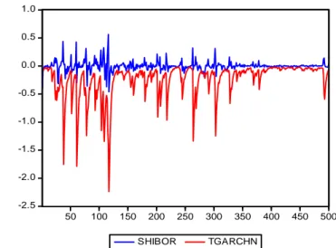
-2.5 -2.0 -1.5 -1.0 -0.5 0.0 0.5 1.0 50 100 150 200 250 300 350 400 450 500 SHIBOR TGARCHN
Figure 6.2.2Result of VaR by using TGARCH model under normal distribution
-.8 -.6 -.4 -.2 .0 .2 .4 .6 50 100 150 200 250 300 350 400 450 500 SHIBOR EGARCHN
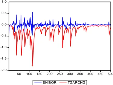
36 -2.0 -1.5 -1.0 -0.5 0.0 0.5 1.0 50 100 150 200 250 300 350 400 450 500 SHIBOR TGARCHG
Figure 6.2.4Result of VaR by using TGARCH model under GED distribution.
-1.2 -0.8 -0.4 0.0 0.4 0.8 50 100 150 200 250 300 350 400 450 500 SHIBOR EGARCHG