A STUDY OF MODELLING THE
ENERGY SYSTEM OF AN ICE RINK
SPORTS FACILITY
Modelling the heating and cooling of ABB arena syd and implementation of
renewable energy sources using TRNSYS
PHILIP LIND
School of Business, Society and Engineering Course: Degree project energy engineering Course code: ERA403
Credits: 30hp
Program: Master of science in engineering energy systems
Supervisor: Maher Azaza Examinor: Ioanna Aslanidou Costumer: Maher Azaza, MDH Date: 2018-06-07
Email:
ABSTRACT
Environmental issues are important challenges for today’s society. Lots of the energy used by humans comes from fossil energy sources resulting in the environmental threats. A
considerable amount of this energy is used in the building sector. Industrial buildings and sports facilities are large users of energy and thus becomes very interesting in an
optimization point of view. Modelling of the systems allows for cheap and effective optimizing of the energy usage and effectivity measures can be investigated and
implemented. This study creates a model of the indoor ice rink arena of ABB arena syd in Västerås using TRNSYS as the main software for simulation. Focus is placed on the heating of the arena through heat pumps and district heating, and cooling of the ice in the arena using cooling machines. The effect of PV as well as a battery storage in the arena is also investigated as an effectiveness scenario. The results from the study revealed that it is possible to simulate the heating demand for the arena, accurately identifying the normal demand as well as the instances when the demand peaks and the magnitude of the peaks. It is also possible to simulate the cooling demand for the ice over extended time periods. However, this study could not identify the peaks for cooling demand. It is also beneficial for the system to install PV, but not a battery storage. With current price levels for electricity it is however not a very beneficial deal. With higher electricity prices the investment is preferable. The study also concludes that TRNSYS can be used for modelling an ice rink sports arena, however it leaves room for improvement on that aspect.
PREFACE
This study is a master thesis work at the program “Master of Science in Engineering- Energy systems though at Mälardalen University in Västerås.
It is created to be used to investigate the energy system of ABB arena syd and do energy efficiency measures to the arena and other arenas similar to it.
Special thanks to Björn Sandvall working at Arvid Svensson which are the owners of the arena. Björn has helped med a great deal by showing the facility, explaining how it works and providing med with information.
My gratitudes to Anton Eskilsson for providing me with consumption data for the arena as well as additional information about the arena and its events.
I want to thank Maher Azaza for support throughout this study. Help with simulations and usage of the software amongst much else
Ioanna Aslanidou for her support and input.
And finally, Douglas Eriksson with his sister project. He has been an invaluable asset when it comes to discussing ideas and concepts.
Västerås in June 2018 Philip Lind
SUMMARY
The world needs to change the way energy is used to meet the present and developing environmental threats in the world. The building sector is a large user of energy on a global scale. To effectively analyse the energy flows and the effects of different energy efficiency measures in an economical way it is necessary to have a simulation model of the building and its components. One software for doing these kinds of simulations is TRNSYS.
Industrial buildings with high demands on heating and cooling for different purposes are very interesting building types to investigate due to their large loads. Similarly, sports facilities such as indoor ice rinks have large energy demands for purposes such as having a quality ice situated in an area which should be pleasant for an audience.
ABB arena syd is such a facility located in the Swedish town of Västerås.
The goal of this study is to analyse if TRNSYS is a good software for doing models of sport facilities with ice rinks using ABB arena syd as a template. The other goal of this study is to investigate and propose energy efficiency measures for the facility in form of renewable energy sources and energy storage units.
Using information about the arena from a previous energy mapping study as well as contact with the manager of facility a template for the model and its specifications is created. A model of the system is designed in Sketchup with TRNSYS extension, TRNbuild and TRNSYS. Emphasis is placed on the cooling machines and the heating to match the
magnitude and behaviour of the simulated consumption to measured values. A radiant floor is used to transfer heat away from the ice floor by flowing a brine through it. The brine goes to cooling machinery which transfers the heat either to a nearby river or (when there is heating demand in the building) to a heat pump which is used for heating of the arena. The heat pump is complemented with district heating in radiators. The district heating is also used to hot tap water as well as heating of the floor under the ice to prevent permafrost. Simulations are done for the model and the results are compared to the measured values. The model is then modified to match the actual demands in the arena.
When the model is created the simulated consumption-data is used in conjunction with the simulated PV data to optimize the amount of PV power to be installed and the capacity of the battery for electricity storage.
The showed showed that it is possible to model an ice rink sports facility using TRNSYS, however it is not an optimal tool for the purpose. The model could replicate the heating demand for the arena to a large degree. Also cooling of the ice was possible to simulate with accurate results for monthly and yearly values. However daily values showed a much larger variance. This is expected to be due to different unforeseen loads on the ice in shape of refurbishing of the ice, human activities heating the ice as well as thermodynamic properties of the ice and the surrounding air.
Installing PV has a positive economic impact on the system, especially if electricity prices will increase. However, the study concluded that installing a battery is not beneficial.
CONTENT
1 INTRODUCTION ... 1 1.1 Background ... 1 1.2 Aim ... 2 1.3 Research questions ... 3 1.4 Delimitation ... 3 2 METHOD ... 4 2.1 Literature study ... 42.2 Contact and visits ... 4
2.3 Data analysis ... 4
2.4 Modelling ... 4
2.5 Validation ... 5
2.6 Economy and sizing of the PV and battery... 5
3 THEORETICAL FRAMEWORK/ LITERATURE STUDY ... 5
3.1 Ice rinks and building simulation ... 6
3.1.1 Validation of simulation ... 7
3.2 Heat pumps ... 8
3.3 PV ... 8
3.4 PV and HP system combination ... Fel! Bokmärket är inte definierat. 3.5 Energy storage and peak shaving ... 9
3.6 Energy in Västerås ... 9
3.6.1 Electricity ... 9
3.6.2 District heating ... 10
3.6.3 TRNSYS ... 10
4 CURRENT STUDY ...10
4.1 ABB arena syd ... 10
4.1.1 Cooling ... 12
4.1.2 Heating ... 12
4.1.3 Ventilation ... 12
4.1.4 Scheduling ... 13
4.2.1 The building ... 13
4.2.2 Weather ... 15
4.2.3 District heating system ... 15
4.2.3.1. HOT WATER ...16
4.2.3.2. FLOOR HEATING ...16
4.2.4 Ice rink cooling system ... 16
4.2.5 Heat pump ... 16
4.2.6 Ventilation ... 16
4.2.7 Electrical appliances ... 17
4.2.8 Scheduling of different activities ... 17
4.2.9 Model validation ... 17
4.3 Applications of energy optimization ... 17
4.3.1 PV ... 18
4.3.2 Battery ... 19
4.4 TRNSYS model and components ... 20
4.5 Economical optimization of the PV and battery ... 21
5 RESULTS ...22
5.1 Validation of model ... 23
5.1.1 Simulation of total heating ... 23
5.1.2 Simulation of Cooling machine power ... 27
5.1.3 Net cash flow of PV investment... 30
6 DISCUSSION ...32
6.1 Model validation ... 32
6.1.1 Heating ... 33
6.1.2 Cooling ... 33
6.2 Evaluation of the PV and the battery ... 33
6.2.1 PV ... 34
6.2.2 Battery ... 34
6.3 Evaluation of TRNSYS ... 34
7 CONCLUSIONS ...35
8 SUGGESTIONS FOR FURTHER WORK ...35
REFERENCES ...36
LIST OF FIGURES
Figure 1 Outside the arena ... 11
Figure 2 Model exterior ...14
Figure 3 Model interior ... 15
Figure 4 TRNSYS model ... 20
Figure 5 Temperatures 2015 ... 22
Figure 6 Temperatures 2016 ... 22
Figure 7 Heating 2015 ... 23
Figure 8 Monthly heating comparison 2015 ... 24
Figure 9 Heating 2016 ... 25
Figure 10 Monthly heating comparison 2016 ... 26
Figure 11 Cooling 2015 ... 27
Figure 12 Monthly cooling comparison 2015 ... 27
Figure 13 Cooling 2016 ... 28
Figure 14 Monthly cooling comparison 2016 ... 29
Figure 15 Cash flow standard ... 30
Figure 16 Cash flow increased electricity price ... 30
Figure 17 Cash flow decreased initial investment ... 31
Figure 18 Cash flow decreased investment increased electricity price ... 31
Figure 19 Cash flow interest rate ... 32
LIST OF TABLES
Table 1 Electricity price 2016 ... 13Table 2 Model dimensions ... 13
Table 3 PV data ... 18
Table 4 Electricity certificate 2015 ... 18
Table 5 Electricity certificate 2016 ...19
Table 6 Monthly heating comparison 2015 percentage ... 24
Table 7 Monthly heating comparison 2016 percentage ... 26
Table 8 Monthly cooling comparison 2015 percentage ... 28
NOMENCLATURE
Symbol Description Unit
E Energy kWh P Power W Q Heat kJ/kg W Work kJ/kg
ABBREVIATIONS
Abbreviation DescriptionCaCl Calcium Chloride- Cooling media used in ice rinks
COP Coefficient of performance
CVRMSE Coefficient of Root Mean Square Error
EPBT Energy Payback time- A KPI indicating how long it takes for an energy harvesting unit to supply the equivalent amount of energy necessary for its production
EU European Union
GHP Ground-source heat pump
HP Heat Pump
KPI Key Performance Indicator
MBE Mean Bias Error
MToe Mega tones oil equivalents- Energy unit related to the energy content in oil.
PV Photo voltaic- the process which converts the energy from solar radiation into electricity, also known as solar power.
1 INTRODUCTION
This study will investigate the energy system of ABB arena in Västerås. Initially a model of the system will be constructed in TRNSYS. The model is to behave like the real building. This will be followed by implementation of renewable energy in terms of solar panels as well as ground source heat pumps.
1.1 Background
Earth is threatened by numerous hazards such as deforestation, pollution and climate change amongst others. This is caused by human overconsumption of its resources (WWF, 2018a). At present humans use 150% percent of earths capacity to regenerate its resources (WWF, 2018b) one of the many things that is overconsumed by the human race is energy (Giljum et al., 2009). In 2016 the total energy consumption in the world was 13276 Mega tones oil equivalents (MToe), where only 1330 MToe originated from renewables (including hydropower). This is only 10 % of the total (BP, 2017).
Due to the ongoing climate changes of the world the Paris agreement was created with the initial goal to cap the global warming to 2 degrees Celsius above the global average
temperature in pre-industrial age. A further goal is set to limit that temperature to 1.5 degrees (UNFCCC, 2018). Other projects are simultaneously fighting the environmental effects of dirty energy use in the world by trying to achieve net zero buildings by 2050. Net zero buildings are buildings that has a total of net zero carbon emissions. By the definition a net zero building is “A highly energy-efficient building with all remaining operational energy use from renewable energy, preferably on-site but also off-site production, to achieve net zero carbon emissions annually in operation” (WorldGBC, 2018). It is possible to utilize the
beforementioned applications on a wide range of building, from residential to industrial types of buildings (Swinter, 2016)
With the building sector being the largest fraction of the worlds energy usage it is of great importance to properly be able to forecast the buildings energy demand and plan accordingly (Lü, Lu, Kibert, & Viljanen, 2015). The study by Lü et al. investigates a method of using a combination of physical properties of the building and statistical consumption data from the building to be able to predict the energy demand more accurate for a sports facility in Finland which amongst other houses ice hockey and swimming pools. Another study made by
Grolinger et al (2016) also concentrates on building energy prediction. However, this study uses smart meter data and the building type investigated is event-based facilities. Using smart metering and data learning the study could predict the energy demand to a large extent.
With annual consumptions ranging from 800 000- 2 400 000 kWh/year for cooling, heating, etc. with the normal being about 1 500 000 kWh/year (Nichols, 2009) ice rink arenas are very energy intensive types of buildings where optimization of the system can have a large impact on the energy consumption. Most energy used in these systems is used for heating and refrigeration. For systems of lesser efficiency, it is observed that the heating is the major user of energy with a demand of 42% of the total with 23% demand for the refrigeration. In more efficient system the refrigeration stands for 42% of the total energy demand with heating at 11% and lighting 21%. The cooling and heating demand is interconnected in the system, with a higher ambient temperature in the arena it is necessary to have a larger refrigerant load in order for the ice not to melt, whilst the inverse obviously applies (MGE, 2018).
A study done by Kuyumcu and Yumrutas (2017) showed that the waste heat from an ice rink system was able to act as a heating source for large swimming pools. The study also discussed the pros and cons of higher COP, with higher COPs it is found that the cooling of the ice rink was not necessarily sufficient to meet the heating demands of the swimming pools. The study also gave input to ice rink arena optimization considering the roof. The optimal ceiling insulation was found to be of 3 cm and it was suggested to coat the ceiling with aluminium foil or paint it with metallic paint to decrease the emissivity of the ceiling.
With all these challenges for the future it is necessary to manage our energy usage and behaviour. One of the tools for this challenge is being able to predict the energy demand for our buildings. One way to do so is by creating models of the buildings in simulation software. Further on, with well-made models it is possible to investigate the potential for different energy optimization actions and energy production units. Ice hockey rinks with large demands on heating, cooling and ventilation are very energy intensive types of buildings, in some ways very similar to industrial buildings. Buildings with these characteristics offers great potential for optimization which is necessary to maintain and improve the life standards of future population of the world.
1.2 Aim
The purpose of this study is to develop a model capable of simulating the behaviour of a sports arena with an ice rink using the software TRNSYS.
Further investigations are to be made on implementation of renewable energy and energy efficiency measures to the system, resulting in a lower operating cost with profit for the environment as well.
The model is also to be able to be used as a framework model for further investigations on the arena, similar arenas and also industrial buildings och similar charcteristics.
1.3 Research questions
How can an ice rink arena be modelled effectively using TRNSYS?
What source/combination of sources of renewable energy and storages will benefit the studied system the most?
1.4 Delimitation
This study is limited to investigations on ABB arena syd. The new instalments that will be investigated are limited to photo voltaic (PV) and a battery storage for electricity. The focus of modelling the system components will be on the cooling of the ice as well as the heating of the building. The simulations will be conducted on hourly intervals of an entire year for both 2015 and 2016. The data will then be summarized and investigated for daily basis. The study is limited by the timeframe of the work.
2 METHOD
The methods used in this study is divided in literature study, contacts and visits at the facility, modelling, simulation and data treatment.
2.1 Literature study
The method used in this study is initially a literature study conducted to obtain crucial detail information about the subject investigated as well as investigating what current research is conducted on the subject.
2.2 Contact and visits
Björn Sandvall working at Arvid Svensson which are the owners of the facilities and handles the operation of the arena was contacted and consulted throughout this study to obtain more detailed information about the facility. Further on a visit to the arena was made to obtain a better understanding of the facility, the visit was guided by Björn. Björn also provided the study with blueprints of the arena as well as relevant case studies conducted at the arena and its systems.
2.3 Data analysis
Data is obtained for the historical consumption of the facility through Anton Eskilsson that has previously been studying the arena. The data is composed of heating consumption, electricity consumption for cooling and electricity consumption for other appliances. The data is used as reference to the simulation data allowing for validation of the final results. Further on the data is used to indicate what the max loads, min loads and operational periods are.
2.4 Modelling
A model of the building is created in Sketchup with the TRNSYS 3d plugin where emphasis lies on the interaction of the ice rink with its surroundings as well as the shell of the arena. The model is exported to Simulation studio in the TRNSYS software for further
modifications. Using TRNBuild the physical characteristics of all zones and their construction elements are specified.
The building model is then used in TRNSYS and other components are connected to it. A concrete slab for cooling is used to transfer heat to the iced area inside the arena. This slab is cooled by a heat pumps created according to specifications of the actual heat pumps. These
are the cooling machines in the system. The working media for the cooling of these slabs are calcium chloride. The waste heat from the heat pumps cooling the ice is used to a second heat pump that is used for heating the arena. A separate heating system using district heating used for supplemental heating of the locker room and providing extra heating power to the system is installed as well. For specific events with higher temperature demands the heating in the arena is increased to a temperature setpoint of indoor climate, which is the same as in the changing rooms.
The input to the model is supplied through an energy plus weather file with temperatures and solar irradiation to the building.
PV is also installed to the system as well as a battery and inverters to simulate the impact of implementing this scenario.
2.5 Validation
By comparing the demand for the simulated system to the actual consumption data the model is further modified to replicate the behaviour of the real arena. To increase the accuracy of the model the technical specifications of the machinery is modified.
2.6 Economy and sizing of the PV and battery
The final step of the work is top optimize the sizing of the PV with economic constraints. Using the production output for the PV from TRNSYS the sizing is done in Excel. By
accounting for the prices for bought and sold electricity, the load, the production, and other economic aspects such as economic support for the PV installation and production is accounted for.
The value of the investment is then calculated using the net present method and an objective function is created to maximize the revenue of the system by changing the amount of
installed PV power as well as battery capacity.
3 THEORETICAL FRAMEWORK/ LITERATURE STUDY
3.1 Ice rinks and building simulation
Karampour gives an extensive overview of the construction and equipment in ice rinks as well as investigations on energy efficiency measures of the systems (Karampour, 2011). On
average the major consumer in an ice rink facility is the ice machine which uses 43 % of the total energy. The cooling demand is followed by the heating demand which on average is 26 % of the energy. In third place is lighting with 10 %. There are different ways of cooling the ice, either using a direct system or indirect or a combination of them both. The Direct system directly uses the area cooled by the ice as an evaporator before being compressed in the heat pump again. The indirect system uses two separate circuits for cooling. The traditional heat carrying media is used limited in the heat pump. The evaporator is a heat exchanger
connected to a secondary fluid system which is the one cooling the ice. The benefit of using the indirect system is that it limits the amount of cooling media used by the heat pump. This is good since this media usually is very harmful to human health and/or the environment. For the indirect system a heat carrier called brine is used in the loop adjacent to the ice. The brine solution is usually made of either calcium chloride or frezium. The heat transferred from the ice can be utilized to a large extent with clever energy efficiency measures reutilizing the heat to the ventilation or floor heating, to mention some applications. The ice sheet and corresponding slab and floor characteristics have several different layers. On top there’s the ice which is cooled by a concrete slab directly below it. It is in this concrete slab that the brine passes through. Under the cooled concrete slab there’s a layer of insulation. Below the
insulation there’s a heated concrete slab. This is installed to avoid permafrost under the ice. The heated concrete slab lies on top of a base layer of sand and gravel. The bottommost part is a water drain.
There’s several different types of heat transfer on the ice according to Karampour. Convection to the surrounding air (which is usually warmer than the ice) is a main contributor. The amount of convection is dependent on several factors, such as temperature difference between the two layers, wind speed and humidity. The humidity leads to the next heat transfer, condensation. The moisture in the air condensates to the colder ice sheet, thus releasing heat to the ice. Radiation is also an important factor for heat transfer. A lot of radiation comes from lighting in the arena, but also the emissivity of the ceiling in the arena have large impact. The final part of the heat transfers is conduction of different origins. Ice resurfacing (when the ice surfacing machines are applying hot water to the ice), brine pump work and skaters are some of the factors leading to increased cooling demand of the ice due to conduction.
Considering the indoor climate of the arena there are dehumidification units. There’s two common methods for dehumidification according to Karampour. The first lowers the
temperature of the air below the dewpoint of the moisture in the air, thus condensing it away. The other method utilizes some type of chemical, silica gel for example, that absorbs the moisture from the air.
Mun and Krarti (2011) creates two simulation models for controlling the ice temperature of an ice rink. The two methods used are brine temperature control and ice temperature control. The brine temperature control shows a small saving in energy, but the desired ice
temperature fluctuates more. To validate the simulation models conducted in Energy plus the authors creates a reference system operated laboratory conditions. The study concludes that the, very small, gain from using brine temperature control is diminished by the gain of the constant quality of the ice obtained through ice temperature control. This is in line with the normal practices in newer ice rinks where ice temperature control is most commonly used. Good et al (2007) investigated a multisport facility with several ice rinks in Canada. Excess heat from the cooling of the ice rinks was used in an additional heat pump to harvest more usable heat. The study came up with several different energy efficiency measures such as using a buffer tank for the heat from the heat pumps, correct dimensioning of the heat pumps, potential for building envelope as well as lighting upgrades to mention some.
3.1.1 Validation of simulation
Coakley et al investigates how to match simulated values for a buildings energy usage to actual data of the usage. The study gives guidelines for calibrating the model and calculating KPIs to be used to validate the accuracy of the model according to different standards.
Amongst others it uses the ASHRAE guideline for Means Bias Error (MBE) (Coakley, Raftery, & Keane, 2014).
𝑀𝐵𝐸 =∑ (𝑠 − 𝑚 )
∑ 𝑚
The Study concludes that the uncertainties in simulation models can be derived to the following points.
Standards- There’s a lack of modelling standards and how to handle the uncertainties arising with modelling.
Expense- It requires a lot of time and instruments to measure, create and validate a model.
Simplification- To create a perfect model there’s an astonishing amount of data necessary as input, these can be hard to find, if even possible. Thus, resulting in simplifications of the model instead.
Inputs- Due to the reasons mentioned in the simplification section the modeler needs to make good assumptions of the input to create a valid model.
Uncertainty- Due to assumptions made for each specification, it is hard to precise where the model turned faulty, due to errors accumulating and eliminating each other.
Identification- When modelling there’s numerous tweaks made by the programmer in based on judgement and/or expert knowledge. This procedure is often not very well documented.
Automation- Due to the vast amount of human input it is recommended to use automatic programming. However, due to the needs of a lot of factual knowledge it might not be so easily done.
Egan et al tried to precise how to be able to diminish the variation from simulation models and real life examples by defining a useful minimal-set of input data for the models (Egan et al., 2018). The study emphasizes on Irish residential buildings ranging from detached houses to apartments. The input is weighted in accordance to impact for the different buildings, thus the most important in one case is not necessarily the most important factor in another case. The study aims to diminish the element of uncertainty in models due to assumptions by informing which parameters are most important for each specific case. For the cases studied it is observed that the setpoint temperature and air change rate is major contributors and crucial to get correct for an accurate model of a residential building. Hong et al came up with a different solution to the same problem, using an optimization algorithm to calibrate the model (Hong, Kim, Jeong, Lee, & Ji, 2017). This resulted in a decrease in the CVRMSE from 18.10 to 12.62 %.
3.2 Heat pumps
Urone et al gives the following explanation to the basics of heat pumps (Urone, Hinrichs, Dirks, & Sharma, 2018). The basics of a heat pump (HP) is a closed system with a cooling media as the working fluid. The fluid enters a hot reservoir at low pressure. The working media has a very low evaporating temperature compared to water, thus it is possible to achieve evaporation and superheating at very low hot reservoir temperatures. The media is then compressed through a compressor before entering the condenser where heat is
extracted to the surrounding cold reservoir. After the condenser the media passes through an expansion valve to decrease the pressure before entering the evaporator once again. Due to the free energy obtained from the hot reservoir (usually from the outside) the system can create a larger energy flow to the area of heating than what is applied to the system through the compressor (which is the energy payed for). The energy gained for each unit of energy inserted to the system through the compressor is called COP (Coefficient of performance) which is a KPI of the system performance, it is calculated accordingly.
𝐶𝑂𝑃 =𝑄 𝑊
3.3 PV
PV installations have shown a beneficial energy payback time (EPBT) of 2-6 years in china depending on where the installations where made (Y. Fu, Liu, & Yuan, 2015). This is based on the results of the primary energy input in the production of the PV which is 12.61 MJ/kWp. Kannan et. al. (2005) concluded that PV is not economically preferable compared to fossil fuel alternatives in Singapore. However, with an environmental aspect included in the investigation the PV would stand a much better chance. It is also pressed on the fact that fossil prices and political aspects concerning the environment might change this.
By combining electricity obtained through a PV system to drive a HP system it is possible to obtain a very efficient system for heating, especially compared to electrical heaters (Omer, 2008).
3.4 Energy storage and peak shaving
Peak shaving is a topic which becomes more and more interesting. It is a way of distributing your energy demand from periods of high demand to periods with lower demand. The result of this can be substantial monetary savings for the consumer. It is discovered that 25% of commercial energy costumers in the united stated would benefit from different peak shaving actions. Some of the tools available for peak shaving is utilizing storage units to shift the load from one instance to another (MicrogridNews&Insights, 2017). Further on the use of storages allows for lesser dependency on the grid in case of sudden supply disruptions (Dunn,
Kamath, & Tarascon, 2011) Battery storages are usually configured either for power or for energy. When configured for power the batteries can release a large amount of energy very quickly, this demands a high inverter to battery ratio. When configured for energy instead the batteries release an even stream of energy for a longer duration and the inverter to battery ratio is then low (GE, 2018). At present there are three different types of thermal storage partially available to the power sector. They are sensible heat storage (which is the presently most available types), latent energy storage and thermal-chemical heat storages (Harvey, 2017).
3.5 Energy in Västerås
Mälarenergi is the main supplier of energy in the city of Västerås (Mälarenergi, 2018b). The company profiles itself as an environmental conscious company with the goal of reaching 0% use of oil and coal in their district heating by 2020 (Mälarenergi, 2018a).
3.5.1 Electricity
Mälarenergi offers four types of electricity packages for their customers. The hydropower package, which consists of 100% hydropower (Mälarenergi, 2018c). The wind power package which consist of 100% wind power. The renewable package which consists of 100%
renewable, however not defined what this exactly consists of. The last package is a mix of fossil energy including peat which corresponds to 48% of the energy, nuclear power for 35% of the energy and 17% percent comes from renewable energy. All packages except the last emits 0g CO2/kWh and no nuclear fuel. The last emits 349,1 g CO2/kWh and produces 1,06 mg nuclear waste/kWh. The total mix for the electricity production consists of 54%
renewable energy, 27% fossil energy including peat and 19% nuclear energy. The corresponding emissions are 192,5 g CO2/kWh and 0,58 mg nuclear waste/kWh.
3.5.2 District heating
The energy mix of the district heating that Mälarenergi provides consists of 57% recycled waste, 35% renewable energy, 4% fossil energy and 4% peat. The resulting CO2 emissions from the district heating is 85,6g CO2/kWh (Mälarenergi, 2018d)
3.5.3 TRNSYS
TRNSYS is according to the corporation itself a flexible simulation software primarily used for investigation of the performance of thermal and electrical energy systems. The software is comprised of two different parts with the first being the engine that utilizes the input to solve the problem. The second is the large library of precomposed models of units ranging from small components such as pumps to entire multizone buildings. The models are user modifiable to match the demand of the user (TRNSYS, 2018).
4 CURRENT STUDY
In the following section the investigated system will be described. It is followed by the
modelling done in the study. The last part is the validation method used for the data obtained through the simulations.
4.1 ABB arena syd
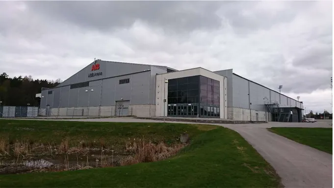
ABB arena syd, Figure 1, is one of the most modern arenas for bandy in Sweden. It is located just outside central Västerås in Sweden in a sports arena complex called Rocklunda
Figure 1 Outside the arena
The arena is 136 meters long 100 meters wide and 21 meters. The heart of the arena is the ice rink, which is cooled to a temperature of -7.5 degrees Celsius (Sandvall, 2018a). The ice sheet is approximately 3-4 cm thick. Depending on the actions going on the ice there is different cooling loads, for example when the ice is refurbished hot water is applied to the surface of the ice which increases the overall temperature. This needs to be countered with increased cooling. The cooling is supplied with three cooling machines of indirect type. The cooling machines are heat pumps using ammonia as working media. The system is of indirect type, which means a separate heat carrier is cooled at a heat exchanger from the cooling machines which in turn cools down the ice. The working media in the secondary circuit is calcium chloride (CaCl). Pipes are installed underthe ice in plastic tubes carrying the CaCl. The temperature inside the arena is set to 6 degrees Celsius. In the changing rooms the temperature is to be at room temperature, 16-20 degrees (Sandvall, 2018a). The locker rooms are the only actual closed rooms in the arena, all else is a big open zone. There’s also a loge which has heating, the loge is however totally open and exposed to the rest of the arena. Heating in the arena is through the ventilation which is applied through ducts running along audience platform (Sandvall, 2018a). In the past the heating was supplied through district heating. However, a heat pump was recently installed which reciprocates the heat from the cooling machines to heat the building. The district heating is still in use for peak loads as well as for heating the cafeteria.
Attempts have been made with installing PV on the building roof. However, the structure is not able to handle the increased weight load of the PV panels, thus rendering it impossible with PV installation there.
4.1.1 Cooling
Cooling in the arena takes place in form of cooling the ice (Pikkarainen, 2014). This system utilizes the indirect system of cooling with a solution of 25% CaCl (75% water) acting towards the ice. The media is then cooled in cooling machines, heat pumps, acting as the hot
reservoir.
The cooling system is composed of three identical heat pumps using ammonia (R717) as working media (Pikkarainen, 2014). The model of the machines is REF Technology RCA717. The cooling power is 633 kW for each one and the combined condenser power is 2436 kW. The dimensioned heat carrying temperature is 20/27
4.1.2 Heating
The heating to the arena is supplied through district heating as well as reutilization of the waste heat from the cooling machines. The waste heat from the cooling machines are used in an additional heat pump to achieve temperatures suitable for the desired heating
applications. The heat is distributed throughout the sports facility complex, thus not being exclusive to the studied arena. About 50% of the heat from the heat pump goes to heating the air in the ventilation system of ABB arena syd and 5 % goes to preheating the water in the arena. The rest of the energy from the heat pump goes to other buildings in the area. The heat pump is of model FOCS/W/H04101-9604 and uses R134-a as working media (Pikkarainen, 2014). The dimensioned power of the system 1125 kW with a heat carrying temperature of 25/35 with a COP of 5 however, the system is operated at a higher
temperature range of 45/50 and obtaining a COP of about 4.
Under the ice there is floor heating to prevent the occurrence of permafrost in the ground. The power supplied to the floor heating is about 50 kW.
The heat pump has been operated in different manners throughout its lifetime. The initial thought of the heat pump was to deliver the heat necessary for heating ABB arena syd (Pikkarainen, 2014). However, when it was taken into action it was instead mainly used to heat a nearby football arena and keep the field snow free during the winter. This has changed to a present setting of about 50% heat from the heat pump to ABB arena syd and the rest goes to other nearby facilities.
District heating is used for heating tap water, floor heating, heating of the cafeteria and the changing rooms. The district heating also acts as the peak load and backup if the heat from the heat pump is insufficient or not working properly.
4.1.3 Ventilation
The ventilation of the arena is made up of several different ventilation systems. What they all have in common is being FTX systems (Pikkarainen, 2014). The efficiencies of these system are about 70 %.
4.1.4 Scheduling
The arena is mainly used for bandy, this is an activity which does not demand high
temperature in the arena. However, the arena is occasionally used for different activities such as fairs, concerts and other sport activities such as handball, football and e-sport. These activities demand a higher indoor temperature than the usual environment of the arena.
4.1.5 Energy prices
The electricity price for 2016 is given in Table 1 (Sandvall, 2018b). The electricity price includes the electricity price, energy tax and transfer fee.
Table 1 Electricity price 2016 Month Total electricity
price [SEK/MWh] January 729,8 February 633,2 March 655,2 April 582,1 May 607,8 June 726,1 July 647,5 August 656,8 September 648,9 October 690,8 November 708,3 December 669,2
4.2 Modelling
The framework building model is created in Sketchup with the TRNSYS plugin. This model is the modified in detail in TRNBuild. The corresponding loads, mechanics and components of the building is created in Simulation studio.
4.2.1 The building
Using Sketchup and the corresponding TRNSYS plugin the frame for the building is created. The model is created in scale and made up of 5 different zones described in in Table 2. Table 2 Model dimensions
Zone Length [m] Width [m] Height [m] Description
Shell 136 100 20.9/13.5 The exterior of
includes the entire system
Ice sheet 105 64 0.1 Zone
representing the ice on the floor of the shell zone
2 x Changing
rooms 40 9 2 Two changing rooms located
on each long-side of the ice on the shell floor
Ground sheet 136 100 0.1 Additional floor
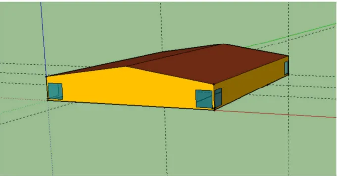
component under the shell Figure 2 shows the exterior of the model created in SketchUp
Figure 2 Model exterior
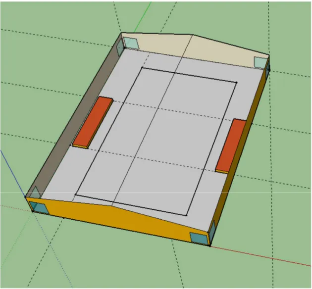
Figure 3 shows the interior of the SketchUp model where the ice rink is visible in the middle of the building and the two heated changing rooms are shown on the sides.
Figure 3 Model interior
The building is then opened in TRNSYS as a “3d Building project”. The properties of the zones are modified. The zone for the ice sheet is given the properties of ice.
The external walls are measured to have a thickness of 30 cm from the blueprints and the wall type is set to be of concrete. The changing rooms wall and ceiling have a thickness of 10cm and constructed of concrete as well.
4.2.2 Weather
Weather data for the current location for the current time of investigation is obtained through shinyapps (2018) in energyplus format. Weather data is only available to March 28 2017.
4.2.3 District heating system
To simulate the district heating demand radiator components are used. These are supplied by a flow of warm water using pumps. The control of the pumps is supplied by PID-regulators.
the temperature drops below the set temperature the pumps are activated and heating of the zones occur.
4.2.3.1.
Hot water
To simulate the hot water usage the consumption data for June (when the cooling machines are turned off and no heating should be necessary) is used. The average daily value during this period is assumed to be representative of the daily tap water usage throughout the year and used as a base load.
4.2.3.2.
Floor heating
The floor heating is assumed to be a constant value of 50 kW. It is a base load solely used during the operational time of the cooling machines when the risk of permafrost is present.
4.2.4 Ice rink cooling system
To allow cooling of the ice a simplified radiant floor (TYPE653) is used as a cooling platform. It is connected to the arena (TYPE56) to fit in between the ice and the slab under the ice. Using a brine of Water and CaCl as working media for the radiant floor.
This cooling circuit is used as the heat reservoir to a cooling machine (TYPE927) which cools the brine cooling the ice floor. The unit is modified in accordance with the data of the actual cooling machines in the arena.
The control of the cooling machines is divided into two different controllers. The seasonal controller which is the dominant controller. This turns the cooling system of when the season is over, and turns it back on when the season starts again. The other controller is a PID controller measuring the temperature in the ice. The setpoint for the ice is as stated -7.5 degrees Celsius. When higher than this the cooling machines starts and cools the ice.
4.2.5 Heat pump
The cooling machine is connected to another heat pump (TYPE927) and transfers the out-data from the cooling machine as in-out-data to the heat pump. The heat pump utilizes the heat to the building and is controlled by a PID controller which is set to 7 degrees Celsius
When heating is deactivated the flow from the heat pumps stops and instead a flow representing outdoor conditions for water is instead used as the hot side for the cooling machine which needs to operate for an extended period of time compared to the heat pump
4.2.6 Ventilation
In the building file ventilation is activated, thus creating an input consisting of the entering temperature of the fresh air. In the simulation studio an equation is created to give the
entering air temperature and acting as a heat exchanger. The temperature difference of the leaving air and the outside air is taken. The difference is multiplied with the efficiency of the FTX which is assumed to have a constant value of X. This is added to the outside temperature creating the temperature of the entering air and the input to the building file.
4.2.7 Electrical appliances
Several electrical appliances except for the heat pump and cooling machines are present in the arena such as ventilation and lighting. Separate data is available for the cooling machines and the lighting, however the ventilation is lumped together with the consumption of TVs etcetera
4.2.8 Scheduling of different activities
Due to the different activities in the arena it is necessary to model a schedule for different operating conditions. The start case is modest normal activity, meaning it’s not a game day nor any other specific activities demanding a higher temperature.
The two scheduled types of cases are the hot and the cold cases. The cold cases are activities with a higher activity than normal for the arena, these are mainly game days for the bandy teams utilizing the arena and other bandy events. The hot events are when activities that demands a higher indoor temperature occurs. For the hot events the temperature setpoint in the building increases to 18 degrees for the day of activity. For the cold events the ventilation is increased.
4.2.9 Model validation
A comparison is made from the simulated data and the actual consumption data of the system to analyse how good of a fit it is.
The initial step of validation is to analyse if the simulated consumption baseline is in the same level as the baseline of the actual consumption data.
The second part is to observe if the curves match each other’s characteristics with increasing and decreasing loads at simultaneous instances.
To obtain a better model the u value of the exterior walls is changed in order for the curves of the simulated values and the actual values to a larger degree match each other.
4.3 Applications of energy optimization
In the following section the data used for creating the PV and battery components are presented as well as how the actual implementation is done.
4.3.1 PV
A PV system (TYPE94a) is created connected to a battery storage (TYPE47a) and an inverter (TYPE48b) who is also in control of charging and discharging the battery.
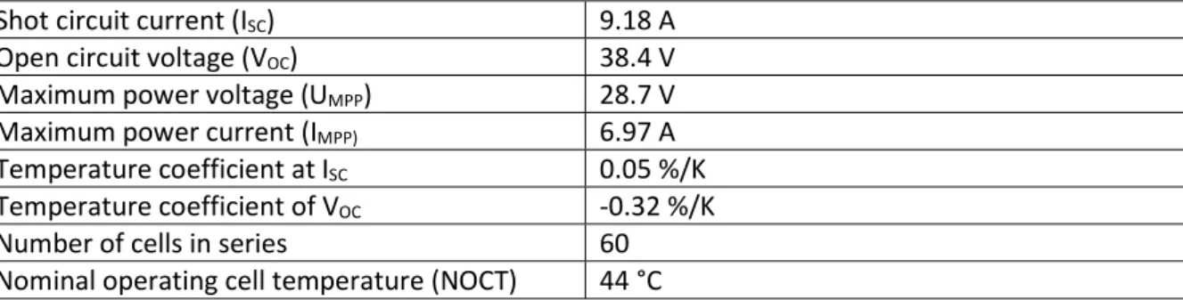
The pv module chosen as a template for the TRNSYS model is the Trinasolar TSM-270PD05 which is a poly-crystalline PV module (Swedensol, 2018). The stats of the module is given by the data sheet (Trinasolar, 2017) and shown in Table 3. The manufacturer guarantees a power output of 80% of the initial value after 25 years.
Table 3 PV data
Shot circuit current (ISC) 9.18 A
Open circuit voltage (VOC) 38.4 V
Maximum power voltage (UMPP) 28.7 V
Maximum power current (IMPP) 6.97 A
Temperature coefficient at ISC 0.05 %/K
Temperature coefficient of VOC -0.32 %/K
Number of cells in series 60
Nominal operating cell temperature (NOCT) 44 °C
The installation cost of the PV varies depending on size of the installation for example. 100 000 SEK is given as key number to the total investment cost for 5 kW of PV
(GreenMatch, 2018). This is in the size of typical household installations. A study conducted at national renewable energy laboratory benchmarking the investment costs for PV of Q1 2017 investigated the different costs for different sizes of facilities (R. Fu, Feldman, Margolis, Woodhouse, & Ardani, 2017). For commercial use with PV installations ranging from 10-2000kW the price was 1.85 USD/Wdc or 2.13 USD/Wac. For utility scale installations (installed power over 2MW) the prices are 1.03 USD/Wac or 1.34 USD/Wdc.
It is possible to obtain an investment benefit for PV installations, of 30% of the total cost, but at most 1,200,000 SEK (Energimyndigheten, 2018a). Electricity certificates is another economical support for production of renewable energy, such as solar power
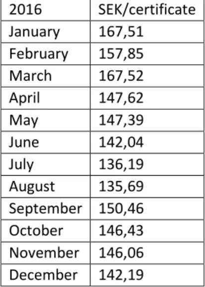
(Energimyndigheten, 2017). The producer is awarded 1 certificate/MWh produced electricity. The certificates can then be sold. Average monthly prices for the electricity certificates is obtained from Energimyndigheten (2018b) and shown in Table 4 and Table 5 for 2015 and 2016.
Table 4 Electricity certificate 2015 2015 SEK/certificate January 172,33 February 164,77 March 187,74 April 153,47 May 152,97 June 155,07 July 153,34 August 151,96
September 160,46 October 168,81 November 169,15 December 164,57
Table 5 Electricity certificate 2016 2016 SEK/certificate January 167,51 February 157,85 March 167,52 April 147,62 May 147,39 June 142,04 July 136,19 August 135,69 September 150,46 October 146,43 November 146,06 December 142,19 4.3.2 Battery
There’s different types of batteries available for use with PV (Energysage, 2018b) . There’s lead batteries, lithium batteries and a new technology of saltwater batteries. Salt water batteries are at present quite untested, being a new technology, but shows significant positive environmental benefits compared to the older counterparts since they do not use any heavy metals. This has given saltwater batteries a high cradle to cradle certification (Solar electric supply, inc., 2018).
Tesla provides a comparatively cheap battery for PV production with an inbuilt inverter with a $/P price of just over 400 USD/kWh (Energysage, 2018a). The tesla Powerwall is lithium ion battery (Energysage, 2018c). The Tesla Powerwall has a capacity of 13.5 kWh for each unit. The maximum discharge is 100% and its in-/out efficiency is 90%. It’s able to handle power flows of 7 kW for short periods and 5 kW for continuous operation (Tesla, 2018)
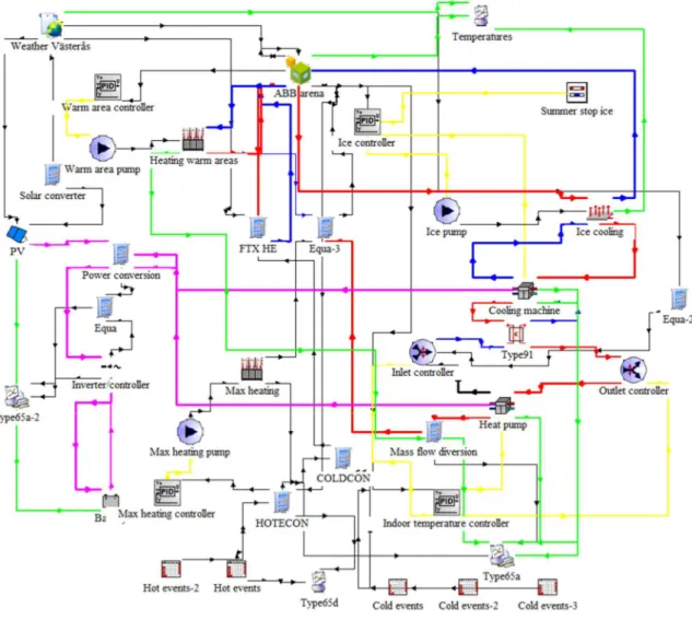
4.4 TRNSYS model and components
The TRNSYS model created of the bandy arena is shown in Figure 4. A list of the different component types is shown in Appendix 1.
Figure 4 TRNSYS model
The models are modified from the actual datasheets to calibrate the model to the consumption data. The modifications will be accounted for in the following section.
The cooling machine is downscaled, however the power to condenser ratio remains the same. The condenser is given the capacity of 812 kW and the corresponding power to the cooling machine is 162 kW.
The cooling slab is dimensioned to fit under the ice rink with a length of 100 m and a width of 60 m. The slab is created of concrete according to the ASHRAE standards.
The heat pump power condenser remains the same of 1125 kW. The power to the heat pump is calculated for a COP of 4 giving 281 kW of electricity.
The heating of the warm spaces which is conducted using a radiator is set to have 15 kW of heating capacity for each of the two changing rooms. The water in the radiators have an incoming temperature of 60 degrees Celsius. The radiators are controlled by the incoming flow of water from a pump. The pump is controlled by a PID regulator that measures the temperature in the changing rooms and operates the pump to reach the setpoint of 20 degrees Celsius.
The auxiliary heating of the arena to support if the heat pump is not sufficient is done by a radiator supplied with district heating water. The control of the auxiliary heating is set to be activated when the temperature drops below 5 degrees Celsius or when it is triggered by the warm events. This is controlled with an equation which then sends the values for heating set point as well as control to a PID regulator which operates the pump supplying warm water to the radiator which has a total capacity of 300 kW.
4.5 Economical optimization of the PV and battery
An excel file is created with input for the load of the system and the PV production exported from TRNSYS. The price that is paid for electricity at Rocklunda arena is obtained from Björn Sandvall and the price for bought electricity is obtained from Nordpol.
The PV adds electricity to the load solely if the load is larger than the PV production. When the PV production is larger than the load the PV charges the battery to the designed
maximum level. However, the charging is not to exceed the maximum charging speed for the design. If there is surplus of electricity it is sold.
The battery is limited by its capacity, its maximum charging and discharging speed as well as maximum and minimum SOC. When the PV is not able to supply enough energy to the load and the battery has an above minimum content the battery is used to supply energy to the load. However, it is not allowed for the battery to discharge faster than the design permits and it is not to have a lower SOC than designed.
The sold electricity is multiplied with the corresponding electricity price as is the bought electricity. The bought electricity is subtracted by the sold electricity giving a result for the electricity expenses.
The profit of PV on an annual basis is calculated and used as a template for all years to come. The profit however decreases in a linear fashion according to the manufacturer (20% drop for 25 years). The incomes are also recalculated according to the net present value. After 15 years a new inverter is installed, the net present value of the expense is calculated. The sum of all the incomes are subtracted by the sum of the incomes giving a total value of the investment An objective function is created to maximize the revenue after 30 years by changing the number of batteries as well as PV modules using numerical solving with the solver in Microsoft Excel.
5 RESULTS
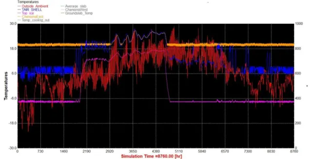
The results from the simulations are shown in the following sections. Figure 5 shows the simulation results of the temperatures, in degrees Celsius, from TRNSYS for the 2015 simulation. The blue line represents the temperature of the air inside the arena. The red represents the outside temperature. Pink is the ice temperature and orange is the temperature in the heated areas.
Figure 5 Temperatures 2015
Figure 6 shows the same results as Figure 5 but for the year of 2016. The colour coding is the same.
5.1 Validation of model
In the following section the validation results for the model will be presented. The measured consumption data will be shown side by side with the simulated values for the investigated areas of the study.
5.1.1 Simulation of total heating
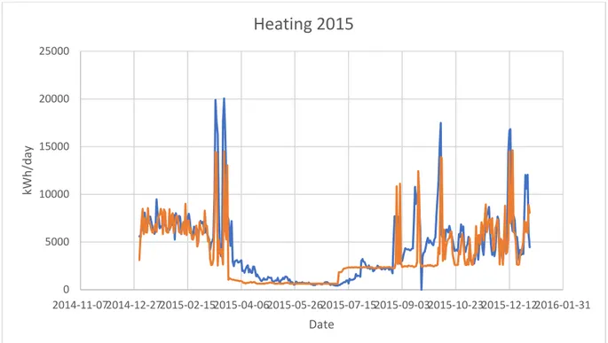
Figure 7 shows the applied heat to the building in the year 2015. The measured values are mainly from district heating with a minor input from the heat pump in late autumn. The heating values include except from heating of the areas heated tap water as well as heating under the ice rink to prevent permafrost.
Figure 7 Heating 2015
Figure 8 also shows the applied heat to the system in the same manner as Figure 7. However, the data is sorted on monthly intervals giving a clearer indication of where the simulation corresponds most to the actual data and where it differs most.
0 5000 10000 15000 20000 25000 2014-11-072014-12-272015-02-152015-04-062015-05-262015-07-152015-09-032015-10-232015-12-122016-01-31 kW h/ da y Date
Heating 2015
Figure 8 Monthly heating comparison 2015
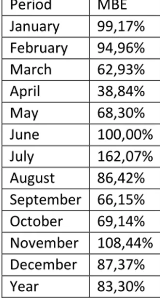
Table 6 Shows the MBE on monthly intervals as a compliment to Figure 8 giving actual numbers on the difference. 100% equals a perfect match. Lower or higher values represent the percentage bellow or above the measured values that the simulated values are. The yearly heat usage for the simulation is only 83 % of the actual demand for the building.
Table 6 Monthly heating comparison 2015 percentage
Period MBE January 99,17% February 94,96% March 62,93% April 38,84% May 68,30% June 100,00% July 162,07% August 86,42% September 66,15% October 69,14% November 108,44% December 87,37% Year 83,30% 0 50000 100000 150000 200000 250000 300000 kW h Month
Monthly heating comparison 2015
The heating for 2016 is shown in Figure 9. The heating for the measured data is supplied through the district heating consumption as well as from the heat pump which is operational by know. The heat pump is however not supporting the heating of ABB arena syd at its full potential. Thus, there’s still a substantial amount of district heating still used in the system. The measured data for the district heating is only available for the first half of the year. Thus, the low to non-present result for the second half of the year for the measured data.
Figure 9 Heating 2016
The heating data sorted for monthly intervals of 2016 is shown in Figure 10.
0 2000 4000 6000 8000 10000 12000 14000 16000 18000 20000 2015-12-122016-01-312016-03-212016-05-102016-06-292016-08-182016-10-072016-11-262017-01-152017-03-06 kWh/day Da te
Heating 2016
Figure 10 Monthly heating comparison 2016
The monthly and yearly overall values for the heating shown in numbers for the MBE is presented in Table 7. The value for the period of January to May is also shown. This is the time before the missing data for the district heating. For this period the simulation only uses 75% of the measured values for the period.
Table 7 Monthly heating comparison 2016 percentage
Period MBE January 82,49% February 100,08% March 79,01% April 77,89% May 83,49% June 237,10% July 2444,13% August - September - October 1307,82% November 262,79% December 209,29% Year 154,18% Jan-May 85,36% 0 50000 100000 150000 200000 250000 300000 kW h Month
Monthly heating comparisson 2016
5.1.2 Simulation of Cooling machine power
The electrical power to the cooling machine in 2015 is shown Figure 11.
Figure 11 Cooling 2015
Also the data for the cooling machine is divided into monthly values to pinpoint where the model is accurate and where it deviates the most. This is shown for 2015 in Figure 12.
0 2000 4000 6000 8000 10000 12000 14000 16000 18000 2014-11-072014-12-272015-02-152015-04-062015-05-262015-07-152015-09-032015-10-232015-12-122016-01-31 kW h/ da y Date
Cooling 2015
Measured data Simulation
0 50000 100000 150000 200000 250000 300000 350000 kW h Month
Monthly cooling comparison 2015
The MBE for the monthly values as well as the yearly overall is shown in Table 8. The total yearly MBE shows that the simulation uses 14% more electricity than what was actually used that year.
Table 8 Monthly cooling comparison 2015 percentage
Period MBE January 188,22% February 113,24% March 0,00% April 0,00% May 0,00% June 131,49% July 82,42% August 89,39% September 89,39% October 96,64% November 140,94% December 126,07% Year 114,44%
The electricity consumption of the cooling machines in 2016 is shown in Figure 13.
Figure 13 Cooling 2016
The monthly division of the data for the cooling machines is shown in Figure 14.
0 2000 4000 6000 8000 10000 12000 14000 16000 2015-12-122016-01-312016-03-212016-05-102016-06-292016-08-182016-10-072016-11-262017-01-152017-03-06 kW h/ da y Date
Cooling 2016
Figure 14 Monthly cooling comparison 2016
The MBE values for the cooling machines is seen in Table 9. For 2016 the total electricity used by the cooling machines is only 5% higher than the measured consumption.
Table 9 Monthly cooling comparison 2016 percentage
Period MBE January 110,71% February 123,99% March 110,34% April 0,00% May 0,00% June 0,00% July 99,76% August 91,67% September 85,23% October 97,07% November 123,53% December 138,11% Year 104,68% 0 50000 100000 150000 200000 250000 kW h Month
Monthly cooling comparison 2016
5.1.3 Net cash flow of PV investment
The sizing optimization of the PV and solar showed that there’s not a benefit of installing a battery in the investigated scenario using yearly net charging for the electricity. Neither was it beneficial with the profit of the PV coming directly from Nordpol spot prices.
The optimization of the PV resulted in the optimal installed power to the system would be 70kW with an installation price of 15.73 SEK/kW using present electricity price and no interest. The cash flow shown in Figure 15 shows that the profit would be marginal with a profit of 2933 SEK over 30 years with an initial investment cost of 1.1 MSEK.
Figure 15 Cash flow standard
With an increase of the electricity price with 50% to an average price of 0.995 SEK/kWh the same system turns out to be more profitable with a revenue of 427,631 SEK over the 30-year period. The result is seen in Figure 16.
Figure 16 Cash flow increased electricity price
-900000 -800000 -700000 -600000 -500000 -400000 -300000 -200000 -100000 0 100000 0 1 2 3 4 5 6 7 8 9 101112131415161718192021222324252627282930 SE K Year
Cash flow
-1000000 -800000 -600000 -400000 -200000 0 200000 400000 600000 0 2 4 6 8 10 12 14 16 18 20 22 24 26 28 30 SE K YearBy decreasing the initial investment to 11,39 SEK/kW and a new sizing optimisation suggested a new installed power of 351 kW to a prize of 4,000,000 SEK to maximize the profit to 920,000 SEK for the period of 30 years. The corresponding cash flow can be seen in Figure 17.
Figure 17 Cash flow decreased initial investment
Increasing the electricity price in addition to the cheaper system further increased the profit to 3,050,000 SEK over the investigated period. It also sped up the payback time of the system as seen in Figure 18.
Figure 18 Cash flow decreased investment increased electricity price
With the beforementioned system utilizing the decreased investment cost and increased electricity price the interest was increased to 6%. With this interest the system is still creating a revenue of 68,000 SEK seen in Figure 19.
-3000000 -2500000 -2000000 -1500000 -1000000 -500000 0 500000 1000000 1500000 0 2 4 6 8 10 12 14 16 18 20 22 24 26 28 30 SE K Year
Cash flow: Decreased initial investment
-4000000 -3000000 -2000000 -1000000 0 1000000 2000000 3000000 4000000 0 2 4 6 8 10 12 14 16 18 20 22 24 26 28 30 SE K Year
Cash flow: Decreased initial investment,
increased electricty price
Figure 19 Cash flow interest rate
6 DISCUSSION
A major problem the study faced was incomplete datasets for each respective year as well as operating conditions of the heat pump was drastically changing throughout the different years, from non-existent, to supplying some heat to the studied system, and at present supplying a large amount of heat to the system.
The studied system is a very complex one considering the timeframe. Some aspects of the system were necessary to leave out due to time/complexity constraints. In combination with the large impact of human behaviour to the system and different operating conditions and cases the results shown are not perfectly calibrated to actual consumption. However, this study be a stepping stone for further investigations of the system and further improvements of the model will most likely result in a higher accuracy.
However, the study is not solely about creating a model for the system. It is also about investigating the software TRNSYS and how suitable it is for modelling a sports facility system.
6.1 Model validation
The model created in TRNSYS shows significant resemblance to the framework system. Especially for total demands for longer time periods. The heating is the most accurate simulation regarding the pattern of the consumption.
-3000000 -2500000 -2000000 -1500000 -1000000 -500000 0 500000 0 2 4 6 8 10 12 14 16 18 20 22 24 26 28 30 SE K Year
6.1.1 Heating
Viewing the results for the heating and looking at Table 6 and Table 7 one might argue that the overall U-value for the building is to low, since the simulation model is on a yearly basis constantly under the measured values. I would however argue the opposite. Investigating Figure 7 and Figure 9 the overall trend of simulation is in line with what is going on in the arena. I would argue that the main reason for the error is caused by the operation of the arena. For the autumn of 2015 the simulation model does not apply any significant space heating except when there are warm events occurring and remains over or at the set temperature. However, investigating the consumption data at these events it is noticeable that heat consumption right after an event drops down to range of the simulated values, however, there’s right after this an increase in heating. This latter increases most likely because the actual temperature in the arena is increased for some reason.
The results for the first part of 2016 gives quite a large deviation from the simulated values. At the instances of the deviations there’s events going on in the arena. However, it is bandy events, which does not demand high indoor temperature as the warm events. However, the pattern of the curve indicates that the arena is repeatedly heated to normal indoor
temperature since the magnitude of the peaks is in the range of the peaks when warm events occurs.
6.1.2 Cooling
The cooling proved hard to give instantaneous correct results with a large degree of
fluctuation going on. One of the problems with the cooling is that it is constantly subject to different heat loads which can be very hard to replicate. The ice sheet is constantly
refurbished, which is achieved with the application of hot water to the surface. This results in an increased demand for cooling of the ice to counteract the heat.
However, the cooling results for 2016 was the only results which are proof of a calibrated model according to ASHRAE.
6.2 Evaluation of the PV and the battery
With the present set of conditions, the PV can be a slight positive impact on the economy of the system. However, if the price level of electricity remains on this low level throughout the life time of the PV, one might suggest that the money could be invested in something with a larger profit. But the present price level of electricity is very low, and the trend of PV prices is negative. Looking at the other economical scenarios it becomes more advisable to use the PV. There’s also the environmental aspect of the PV reducing the emissions otherwise produced in the energy system of Västerås.
6.2.1 PV
The benefit of installing PV is at present unexpectedly low. This is believed to be caused by the quite low cost for buying electricity from the grid. This decreases the incitement for PV installations. However, it is profitable. Especially when investigating scenarios with increased electricity prices. But the manageable interest rate makes it less of an attractive choice if looking at pure monetary revenue. However, since the bought electricity is not of purely renewable origin it is of environmental positive impact with the investment. As shown in other studies PV investments have a relatively low EPBT. And since the investment is profitable it can be considered as an act for the environment as well as being good PR with companies acting for a cleaner energy future, both globally and locally.
6.2.2 Battery
With the concept of net charging for the electricity that Mälarenergi uses it is not a big surprise that using batteries is not beneficial since the storage obtained through the battery has a significant cost, while with net charging the storage is almost unlimited for free. The investigated system really prospers with this kind of system since it produces the most during the summers where there’s not that large of a consumption of electricity in the system. The ability to save the value of this production to the winter months makes the whole concept feasible.
6.3 Evaluation of TRNSYS
TRNSYS with the TESS plugin provides an extensive library of different components to ease the efforts needed for simulation. It takes quite some time to learn how to handle TRNSYS, but when the initial learning is finished it offers a smooth simulation software. All
components come with a detailed description about what they do and how, including the built-in equations in every component. Thus, it is possible to easily verify and replicate the components when wanted to.
What could be better in TRNSYS is that one cannot search for specific components in the library, but you must manually go into the library through several folders to find any specific component. This is initially very time consuming, especially when you are not fully aware where any specific component is located, and some similar components are in different folders. Thus, it is easy to miss components and lose the full potential of the software. Another personal feeling is that the software from time to time appears buggy. It freezes up and shuts down on some instances so you must make sure to always save your work before initializing a simulation. The troubleshooting features of the software leaves a lot left to be asked for as well. The most disturbing is when a simulation starts with getting an error and stops and it is not always possible to open the listing file to see where the error occurs and why. If you have only made one change in the model before the last simulation it is easy to go back and change that specific parameter and the problem should be solved. But when there’s several parameters and perhaps different components involved in between simulations the
problem gets a much larger magnitude. However, this usually does not occur and seems to just be some sort of bug that will be fixed.
One obvious flaw of TRNSYS is that it does not handle the phase change of materials (the ice) which is a crucial component in the system. This should affect the possibilities to create accurate simulation of the ice for example.
7 CONCLUSIONS
The study has been modelling the energy system of ABB arenas syd using TRNSYS. The focus was placed on the heating of the arena as well as cooling of the ice. The potential for installing PV on the arena was also investigated. The conclusions drawn from this study is that TRNSYS can be used to simulate the heating and cooling demand for an ice rink sports facility. The accuracy of the model created in the given timeframe is not to be considered a validated model as much as an indication of the demands for the arena. The complexity of the building and the non-standardized operating procedures of the arena as well as unforeseen events is considered to have played a large factor considering the accuracy of the model. Since a system like this is very complex it is necessary to take emphasis on all details and inputs of the system to create an accurate model. The largest obstacle is the impact of human
behaviour on the system, such as change in operating procedures (when the arena is to be heated for activities demanding a warmer indoor climate) as well as sudden loads which can be hard to predict, such as refurbishing of the ice and its impact on the cooling of the ice. It is concluded that installing PV is most beneficial with high electricity prices. A PV module produces a specific amount of electricity for each year. The higher the electricity price, the higher the benefit of the PV. It is also concluded that using battery storage for the electricity is not beneficial. Especially with the case of yearly net pay for the electricity as is the case in Västerås with Mälarenergi. The system would benefit from the installation of PV however, with present price levels the gain would not be that significant.
8 SUGGESTIONS FOR FURTHER WORK
Further calibration of the system is advisable. Utilizing more inputs is suggested to enhance the accuracy of the model for a better match.