Internalisation of External
Effects in European Freight
Corridors
10
Discussion Paper 2013 • 10
Anna Mellin, Asa Wikberg,
Inge Vierth, Rune Karlsson
VTI, SwedenInternalisation of external effects in
European freight corridors
Discussion Paper No. 2013-10
Anna MELLIN
VTI – The Swedish National Road and Transport Research Institute, Stockholm,
Sweden
Åsa WIKBERG
VTI – The Swedish National Road and Transport Research Institute, Borlänge,
Sweden
Inge VIERTH
VTI – The Swedish National Road and Transport Research Institute, Stockholm,
Sweden
Rune KARLSSON
VTI – The Swedish National Road and Transport Research Institute, Linköping,
Sweden
THE INTERNATIONAL TRANSPORT FORUM
The International Transport Forum at the OECD is an intergovernmental organisation with 54 member countries. It acts as a strategic think-tank, with the objective of helping shape the transport policy agenda on a global level and ensuring that it contributes to economic growth, environmental protection, social inclusion and the preservation of human life and well-being. The International Transport Forum organises an annual summit of Ministers along with leading representatives from industry, civil society and academia.
The International Transport Forum was created under a Declaration issued by the Council of Ministers of the ECMT (European Conference of Ministers of Transport) at its Ministerial Session in May 2006 under the legal authority of the Protocol of the ECMT, signed in Brussels on 17 October 1953, and legal instruments of the OECD.
The Members of the Forum are: Albania, Armenia, Australia, Austria, Azerbaijan, Belarus, Belgium, Bosnia-Herzegovina, Bulgaria, Canada, Chile, China, Croatia, the Czech
Republic, Denmark, Estonia, Finland, France, FYROM, Georgia, Germany, Greece, Hungary, Iceland, India, Ireland, Italy, Japan, Korea, Latvia, Liechtenstein, Lithuania, Luxembourg, Malta, Mexico, Moldova, Montenegro, the Netherlands, New Zealand, Norway, Poland, Portugal, Romania, Russia, Serbia, Slovakia, Slovenia, Spain, Sweden, Switzerland, Turkey, Ukraine, the United Kingdom and the United States.
The International Transport Forum’s Research Centre gathers statistics and conducts co-operative research programmes addressing all modes of transport. Its findings are widely disseminated and support policymaking in Member countries as well as
contributing to the annual summit.
Discussion Papers
The International Transport Forum’s Discussion Paper Series makes economic research, commissioned or carried out at its Research Centre, available to researchers and
practitioners. The aim is to contribute to the understanding of the transport sector and to provide inputs to transport policy design. The Discussion Papers are not edited by the International Transport Forum and they reflect the author's opinions alone.
The Discussion Papers can be downloaded from:
www.internationaltransportforum.org/jtrc/DiscussionPapers/jtrcpapers.html
The International Transport Forum’s website is at: www.internationaltransportforum.org
For further information on the Discussion Papers and other JTRC activities, please email:
TABLE OF CONTENTS
PREFACE ... 4
1. INTRODUCTION ... 4
1.2 Method and limitations ... 5
2. DESCRIPTION OF THE CORRIDORS ... 11
2.1. Oslo–Rotterdam ... 11
2.2 Narvik-Naples ... 13
3. EXTERNAL COSTS BY MODE... 17
3.1 Road ... 17
3.2 Rail ... 18
3.3 Sea ... 19
4. CHARGES AND TAXES BY MODE ... 21
4.1 Road ... 21
4.2 Rail ... 22
4.3 Sea ... 23
5. RESULTS - RATE OF INTERNALISATION BY ROUTE ... 25
5.1 Oslo - Rotterdam ... 25
5.2 Narvik – Naples ... 30
5.3 Comparison between countries ... 35
6. DISCUSSION AND CONCLUSIONS ... 36
7. REFERENCES ... 39
Published references ... 39
Websites ... 40
APPENDIX – SENSITIVITY ANALYSIS ... 42
Oslo – Rotterdam ... 42
PREFACE
This project was conducted and financed upon a request from the Swedish governmental Agency Trafikanalys (Transport Analysis), with a governmental assignment to annually report the rate of internalisation per mode for passenger and freight transport. In its 2013 report, the Agency wishes to show examples of how the marginal costs and the internalising taxes and fees vary within and between European countries. With this background, VTI was given the assignment to analyse ten freight routes in Europe within the Narvik (Norway)–Naples (Italy), and Oslo (Norway)–Rotterdam (the Netherlands) corridors. The corridors were stated in the assignment from Trafikanalys. During the project, two reference group meetings were held with the following participants: Kenneth Wåhlberg (Swedish Transport Administration), Stefan Back (TransportGruppen), Katarina Händel (Swedish Maritime Administration), Gunnar Eriksson (Trafikanalys), Rein Jüriado (Vinnova) and Anders Ljungberg (our Trafikanalys contact). Further, Glenn Håkansson (former truck driver) helped out with selecting the routes for the road transport. The authors would like to thank all participants for their helpful comments. The report was reviewed by Jan-Erik Swärdh, Ph.D., on December 5, 2012 at a public seminar at VTI. The authors made alterations to the final manuscript of the report. Any remaining errors rest with the authors.
1. INTRODUCTION
External effects or externalities “consist of the costs and benefits felt beyond or ‘external to’ those causing the effect” (Anderson, 2006). In the case of transportation, the negative externalities (costs) can take the form of air pollution, noise and accidents. Since external effects do not have a market price, external effects are a form of market failure. Wear and tear of the infrastructure is external to individual drivers and operators, and thus also included in the analysis.
External costs can be internalised in various ways e.g. through regulatory measures, technological development or taxes and charges. Some forms of taxation are more effective than others in internalising costs. For example, fuel tax is effective in reducing CO2 emissions as it will tend to promote technological change to reduce emissions per kilometre travelled as well as reducing the kilometres driven. A fixed, undifferentiated annual tax on owning a vehicle will, on the other hand, be ineffective in relation to reducing CO2 emissions. While it will have some impact on reducing vehicle ownership (and thus indirectly vehicle use), it will not affect kilometres driven by individual vehicles. In this paper the focus is on the “rate of internalisation”. This term is used to describe to what extent the marginal external costs, based on existing regulations and technology (e.g. the European Emission Trading Scheme and emissions classes for road vehicles), are compensated for through charges or taxes. Internalisation at a certain time is thus expressed as the ratio between average charges and taxes on the one hand, and marginal external costs on the other. In this case, a full rate of internalisation would imply that the transport companies are fully charged for the marginal negative effects caused by their transport. If the ratio is below 1, the taxes and charges levied are lower than the existing marginal external costs to society, i.e. there is an under-internalisation. The aim of this project is to study the rate of internalisation of external effects through taxes and charges in two European freight corridors during 2012; for road, rail, and sea transport, respectively. The study is based on two presumed freight corridors, between Norway (Narvik) and Italy (Naples), and between Norway (Oslo) and the Netherlands (Rotterdam).
The analysis is further differentiated on a national level, where each country constitutes one segment of the transport.
1.2 Method and limitations
To address the issue of rate of internalisation, there are two important components, the negative external costs associated with transportation based on existing technology and regulations, and the existing charges and taxes levied in each country on the transportations companies/consumers. Our focus will be on links; consequently, neither external costs nor taxes and charges related to nodes will be considered (ports are seen
as nodes in this study). The external costs that will be treated include air pollution1, emissions of carbon dioxide (CO2), noise, accidents, and the wear and tear of infrastructure. Due to its high level of uncertainty (see Section 1.7), congestion is only considered in our sensitivity analysis. Other external costs, such as the loss of landscape and soil and water pollution, will not be addressed here2.
The starting point is that external costs related to a specific decision should be matched by a charge or tax of the same amount, in order to achieve maximum efficiency in any given activity. In this paper, we focus primarily on the decision to transport one extra kilometre; the marginal cost is, therefore, expressed as the cost per (extra) kilometre and the charge is basically the charge per (extra) kilometre.
The marginal costs are mainly based on data presented in the Handbook on estimation of external costs in the transport sector (CE Delft, 2008), commissioned by the EU, which hereafter will be referred to as IMPACT3. In some cases, other sources are used due to missing IMPACT data. The background of the IMPACT Handbook is a request by the European Parliament in the previous version of the so-called Eurovignette Directive for the Commission to present an analysis of external costs. The report was included in the “Greening Transport Package” issued during the summer of 2008 which also included an updated version of the Eurovignette Directive in which the values presented in the IMPACT Handbook was used.
The report is limited to the use of existing infrastructure with existing vehicles under existing regulations, while the potential externalities of the use of future infrastructure, with future technology and regulations will not be considered. Further, we base our analysis on current state-of-the-art knowledge; since there is more research and knowledge in the area of road traffic, that part of the analysis will be more thorough. It is important to note that only short-term marginal costs will be considered.
The taxes and charges taken into consideration in our analysis are those that are levied depending on the usage of the infrastructure or the vehicle/vessel, i.e. either per kilometre or by the number of passages (see section “Charges and taxes by mode”). The vehicle tax, which is an annual charge, for road transport is used to analyse the difference between domestic and international transport.
The study is limited to one vehicle or vessel type for each transport mode, and the transport is assumed to be unimodal. Whenever possible, we have selected the same, or similar, vehicle types as used by the OECD/International Transport Forum (ITF) in its study on fees and taxes for road and rail (ITF, 2008a and 2008b).
The routes selected within the corridors
In settling on the routes, the considerations obviously vary for the three transport modes represented. Whereas the sea route is quite straightforward, assuming that vessels will choose a fairly straight route from point A to point B, while rail and road traffic must
1 Based on the pollutants considered in CE Delft (2008), the relevant pollutants include particulate matter
consider other factors such as the quality of road or track, which is not always in favour of the straightest route.
It is important to understand that the corridors are in some sense hypothetical, i.e. they are not chosen because these routes represent actual routes for each of the transport modes studied. This paper is an attempt to analyse the possible traffic flows along freight corridors, even though in reality, a vehicle only uses parts of the route in the freight corridor. The routes represent a selection of the main routes for Swedish goods.
Road
To specify the route for the road transport, several different tools have been used. SAMGODS is a tool for freight transport modelling, developed by the Swedish Transport Agencies (Vierth et. al., 2009). Since the Swedish segment contains a great number of details, this tool has been used to select the road routes for this segment. The Swedish routes have as far as possible been selected according to HVN-1 and HVN-2, i.e. the main freight routes as identified by the Swedish Transport Administration (Banverket et al, 2009). However, for roads in other European countries, other tools have been used, such as “Resa mellan” (“Travel in-between”) (2012), Google maps and distance tables. These tools have also been used to calculate the share of motorways and non-motorways. In the north of Sweden, it is common with 2+1 roads, especially along the coast. These roads have a fatality risk similar to motorways (Carlsson, 2009), and might, therefore, be overestimated in the external cost calculations for accidents in instances where these routes have been classified as “other roads” for purposes of using the IMPACT values. On the other hand, if classified as motorways, since the parts that only constitute one lane indicate an increased wear and tear due to rutting (Lunds Universitet, 2013), the cost of wear and tear might be underestimated.
It has also been assumed that as far as possible, the routes follow the TEN-T4 network, and discussions with a truck driver experienced in European driving have confirmed our choice of routes. For estimating the share of our routes that passes through urban and rural areas, the GIS tool developed in the ASSET (Assessing sensitiveness to transport) Project has been utilised (ASSET, 2012)5. These estimates are rather rough and are based on squares of 1km*1km, and might principally affect noise costs which depend on the population density (see Table 3).
Rail
There are currently several projects involving rail corridors in Europe. Some of these corridors already exist, while others represent future corridors (EC Mobility and Transport, 2012). In settling on freight routes, we have used some of the projects mentioned below as a reference for the track sections that are interesting from a corridor perspective. The distances have been calculated by mainly using the SAMGODS model. In cases of uncertainties, distances have been validated against other Swedish sources. The distances for all tracks outside Sweden have not been validated against other sources; hence, the uncertainties for these distances are greater.
4 Trans-European Network for Transport.
Within Europe, there are a number of different rail systems, which are hindering transnational rail traffic. The trains are sometimes forced to change locomotive and/or train driver at the borders. In order for rail not to lose market shares to other transport modes, EU has decided to institute measures to enable transnational rail traffic. The new system is called European Rail Traffic Management System (ERTMS) and is a standardized safety and train control system for European rail. The aim is to standardize all European railways through the ERTMS, but initially, focus will be on a few selected routes (Trafikverket, 2012b). Other projects involving European rail corridors include the TEN-T priority axes, RNE-corridors, CER, and TREND6. Comparing these different approaches has given us a fair idea of the prioritised and most important rail freight routes in Europe (EC Mobility and Transport, 2012).
We have chosen to follow the full extent of the ERTMS Corridor B through Denmark, Austria, Italy, and partly through Sweden and Germany. In Norway, the Netherlands, and partly in Germany, we chose the shortest route by studying rail maps. In Sweden, apart from following the ERTMS Corridor B route whenever possible, we also used common knowledge of the flows of rail freight traffic. In some cases, there were several alternative tracks between cities. In those cases, we consulted infrastructure managers in the relevant countries and studied local geographical characteristics in order to select the most likely route for our freight trains.
Sea
For sea routes, ships are assumed to take the shortest lanes and as far as possible follow the “Motorways of the Sea” routes without making any stops. Motorways of the sea is a concept developed as part of the transportation policy of the European Union to strengthen the network between Member States and to highlight the importance of sea transport. However, in some cases, it has been relevant to the analysis to add stops along the way. In these instances, the “sea-distance” web tool was used to calculate the distances (Sea distances, 2012).
Standardized vehicles, trains and ships
For road transport, the standardised vehicle is a 40 tonne, 18.75 metre long truck of the EURO Class IV, which is the EU standard for vehicle emissions. These assumptions are in line with the standardized HDV (heavy duty vehicle) featured in IMPACT and ITF (2008b). The fuel consumption is assumed to be 0.33 litres per vehicle kilometre for non-motorways and 0.26 l/vkm for non-motorways (HBEFA, 2012). These assumptions7 are used to calculate the diesel tax per vehicle kilometre. The annual amount of kilometres driven for the vehicle is set at 125,000 (ASEK, 2012), and is used to recalculate the vehicle tax and the Eurovignette into a tax per vehicle kilometre.
Following Thompson (2008), we assume a freight train with a gross tonne weight of 960 tonnes. We also assume an electrical locomotive in our main analysis. There is no consensus on how to treat the emission from electric production in the contemporary transport sector. In this study, we have used the valuations and assumptions made in IMPACT; hence, a European mix of electric production is used. For the sensitivity analysis, a diesel locomotive will also be included.
6 RNE = RailNetEurope, CER= Community of European Railways, TREND = Test of Rolling Stock
For sea transport, container feeders have been selected. Since the container can be handled by all modes, a container feeder is a common vessel in short sea shipping that is often used in comparative studies8. The size has been chosen based on two criteria, the most common ship sizes calling on both the ports of Norway and Italy (the Narvik-Naples corridor) as well as Norway, Sweden and the Netherlands (the Oslo–Rotterdam corridor) (Eurostat, 2012), as well as the common ships used in previous studies (e.g. Naturvårdsverket, 2010; Hjelle & Fridell, 2012). The characteristics of the container feeder selected are: 1000 TEU9 with a gross tonnage (GT10) of 13 000 and an assumed load factor of 70 %11. Heavy fuel oil (HFO) containing 2.7 % sulphur is assumed to be used at 80 % and 20 % HFO with a 1 % sulphur content for the Narvik to Naples route, meanwhile for the Oslo–Rotterdam route, only HFO with a 1 % sulphur is assumed to be used (due to ECA regulations on sulphur content, see Section 5.1.3). Tier 112 is assumed for the emissions of nitrogen oxides (NOx) from the vessel for both routes.
For the road routes, there is also a ferry connection in both corridors. For these routes, we assume the use of a RoRo ferry, based on available ships in the NTM13 database similar to those used by the ferry companies operating along these routes, i.e. Trelleborg-Travemünde and Trelleborg–Rostock (TT Line, 2012). The same type of ferry is assumed to operate the Rödby–Puttgarden link. The characteristics of the ferry are the following: 2,200 lane metre, 6,080 deadweight tonnes (dwt) with an assumed load factor of 44 %. HFO with a 1 % sulphur content is assumed, and Tier 1 for NOx emissions.
Sensitivity analysis
We also include sensitivity analyses to test the robustness of our analysis and to deal with such complex issues as congestion.
The following alternatives have been analysed for road and rail transport: Noise cost has been assumed for either all day or all night transport, compared to the main analysis for which an average of the cost valuation for day and night has been assumed.
Due to the specific topographical and meteorological conditions, correction factors for Alpine areas from Lindberg (2006) have been used for the total segment in Austria and 25 % of the Italian segment.
Further, for roads, the Swedish values on wear and tear from IMPACT have been analysed and compared to those for EUR27 used in the main analysis due to the fact that
8 Note that the environmental impact of short sea shipping is strongly dependent on ship type and size. For
cases when small RoRo and container vessels are among those with the worst environmental performance, see Hjelle & Fridell (2012).
9 Twenty-foot Equivalent Unit is a measurement which is equal to the size of one twenty foot container. 10 Gross tonnage= the total of all enclosed spaces within a ship expressed in tonnes, each of which is
equivalent to 100 cubic feet.
11 Conversion factor from TEU to GT is based on Chiffi et al (2007).
12 Part of the MARPOL convention and regulates the allowed levels of NOx emissions from marine engines.
Tier 2 was introduces in 2011, and Tier 3 will be introduced 2016 (IMO, 2008).
13 The Network for Transport and Environment (NTM) is a non-profit organisation, initiated in 1993, aiming
at establishing a common base of values on how to calculate the environmental performance for various modes of transport, http://www.ntmcalc.org/index.html.
IMPACT values assume that variable average costs are a good approximation of the marginal cost. However, this is not the case for countries with low traffic volumes such as Sweden (a further explanation is found in Section 3.1). Also, the lowest fuel tax for each road route has been calculated; with the rough assumption that one tank would be sufficient for the entire trip14. For sea transportation, no sensitivity analysis has been conducted.
Finally, we have addressed the issue of congestion by using different approaches for road and rail. Because congestion is a function of transport demand relative to fixed supply (i.e. traffic volumes in relation to capacity) where demand varies considerably depending on the time of the day, congestion on the roads and the scarcity of track availability is quite specific to location and time. It is common to distinguish between two congestion peaks during the day, i.e. morning and afternoon commuting. Although the peaks vary for different environments, we assume that for road traffic, they are occurring at 7-9 am and 6-8 pm (Christidis and Brons, 2010). Where peaks occur is dependent on the demand in different locations (e.g. commuter traffic in large cities) in relation to capacity (e.g. motorways). It is not obvious that highways would have less congestion than other roads and there is often a correlation between demand and capacity.
The external cost of congestion is the difference between the average time cost of road users and the marginal cost, i.e. since this road user generates delays for all the others (Button, 1993), the external cost of congestion for the last road user consists of the sum of all others. It is also valid to note that there is a congestion cost without pricing and a congestion cost incurred after implementing pricing, i.e. while drivers adjust to new prices, a lower cost relevant to the congestion cost appears. IMPACT assumes a price elasticity of 0.3 when assessing the cost of congestion that arises after a congestion price has been introduced.
To exemplify the cost of road congestion in a corridor analysis, we imagine three methods. We have chosen the first method; the other two are potential developments for future analyses:
1. We assume that a transport starts at a certain hour and after taking into account driving and rest times, it will pass through peaks in the various segments (i.e. the location is not addressed more specifically than by country) before reaching the final destination, an example of a type of transportation that takes into account the time-specific characteristic.
2. The starting hour of the vehicle can be set for several different times of a day (e.g. 06.00 - 24.00), thus making congestion arise on various routes along the corridor. By adopting a distribution of departure times by using the Monte Carlo simulation model, we can study how congestion costs occur at different points along the corridor and then calculate an average congestion cost (e.g. in a study by Christidis and Brons, 2010). 3. The third method is to co-operate with a firm using route guidance systems. Their large databases make it possible to obtain real-time, or at least decent, estimates of the exact location and time for congestion in the road network.
Similar to road congestion, rail congestion is time and location specific. It is, however, hard to find a general rule applicable to all countries. First, data are lacking on the congestion/scarcity on the European railway network. In some countries, congestion
seems to be the heaviest around major cities, while in other countries, track sections between major nodes are more congested. In the sensitivity analysis for rail congestion, we have assumed a worst case scenario in which congestion occurs along the entire route. At some locations along the route, there are special passage fees for peak hours. We assume that trains pass all such locations and are, therefore, charged the maximum congestion charges.
2. DESCRIPTION OF THE CORRIDORS
In this chapter, the two corridors will be presented, as well as the specific routes for each mode of transportation. The term corridor is used in a wider definition which includes the different routes selected for analysis in this study.
2.1. Oslo–Rotterdam
Figure 1 shows the sea, road and rail routes for the Oslo-Rotterdam corridor. The blue line represents the sea route, both for Oslo-Rotterdam and for Oslo-Gothenburg-Rotterdam. The red line represents the route by road, with the ferry connection between Trelleborg and Travemünde, as well as Rödby-Puttgarden, shown as a blue line. The green line represents the rail route, which in large parts is similar to the road route.
Figure 1. The corridor between Oslo and Rotterdam, via Gothenburg
Road
The road corridor starting in Oslo, Norway passes through Gothenburg, Sweden and then runs via either Germany alone or Denmark and Germany before reaching Rotterdam in the Netherlands. The corridor is shown in Figure 1 and is specified in Table 1. For this corridor, we have assumed two different routes. The first route is via the ferry connection between Trelleborg and Travemünde, selected because it is one of the most frequently used freight routes to and from Sweden, and because it provides some resting time for the driver. The second route via the Rödby – Puttgarden ferry link is chosen because it constitutes an interesting example for future analysis when the Fehmarn Belt Fixed Link will have been built.
Table 1. Oslo–Gothenburg–Rotterdam by road
Country Destination Route
Norway Oslo-Svinesund E6
Alternative 1
Sweden Svinesund-Gothenburg E6
Gothenburg-Trelleborg E6/E20/E22 Trelleborg-Travemünde Ferry
Germany Travemünde-Lübeck B75/A226
Lübeck-Hamburg A1/E22
Hamburg-Hengelo E22/E37/E30
Alternative 2
Sweden Svinesund-Gothenburg E6
Gothenburg-Malmö E6/E20
Öresund Bridge Bridge
Denmark Malmö–Rödbyhavn
Rödbyhavn-Puttgarden Ferry
Germany Puttgarden-Hengelo E47/E22/E37/E30
The Netherlands Hengelo-Rotterdam E30/E25
Rail
The rail route between Oslo and Rotterdam starts along the Østfoldbanen between Oslo and the Swedish border at Kornsjö. At one point, the route has two alternative tracks. We have chosen the Eastern, and shortest, alternative. In Sweden, the train passes Gothenburg and follows the West Coast Line (Västkustbanan) to Halmstad, where the route makes a detour in order to avoid the congestion along the line further south. From Hässleholm, the route follows the Southern Main Line to Malmö, and across the Öresund Bridge to Denmark.
The route through Denmark runs through Copenhagen, then across the Danish mainland via the Great Belt Bridge, through the cities of Odense and Kolding to Padborg by the Danish/German border.15
In Germany, the route runs from Padborg/Flensburg, via Hamburg, and turns west, continuing towards Bremen and further to Osnabrück and Bad Bentheim. The great rail terminal in Duisburg was not included since it would constitute a large detour for trains running from Scandinavia towards Rotterdam.
In the Netherlands, the route runs through Hengelo, Almelo,Gouda to finally arrive in Rotterdam. The dedicated freight route, the Betuwe Line, starting from the port of Rotterdam to Germany, was excluded for the same reasons as discussed above regarding Duisburg. Even though a large part of the train freight from the Netherlands to Germany uses the Betuwe Line, it would have meant a large detour in this case.
Sea
For the sea corridor, we have decided to illustrate two routes, one from the port of Oslo directly to Rotterdam and one from Oslo via Gothenburg to Rotterdam. As stated in the corridor specification, because container feeder traffic between Gothenburg and Rotterdam is common, the second route includes Gothenburg. The main maritime traffic flows to and from Sweden and the South of Norway can be seen on Swedish Maritime Administration maps based on AIS-data (SMA, 2012a). These maps show that the main traffic flows pass North of Denmark rather than through the Kiel Canal.
2.2 Narvik-Naples
Figure 2 below illustrates the routes in the Narvik-Naples corridor. The blue line represents the sea route. The red line shows the road route, with two possible routes through Sweden, either via Västerås or via Stockholm, with a ferry connection between Trelleborg and Rostock. The rail route is represented by a green line. Again, even though the rail line features more “detours” than the road, the rail and road routes are fairly similar.
15 An alternative trail would be possible in the future using the Fehmarn Belt Fixed Link. This alternative is,
however, not relevant in this study since the majority of current flows of rail traffic runs across the Danish mainland.
Figure 2. The corridor Narvik-Naples
Road
In order to have all main routes of the freight flows represented, the road corridor from Narvik includes both the route via Västerås and Stockholm. However, there are mainly inbound and outbound transport to Stockholm, i.e. not a great deal of transit transportation. The Swedish routes have as far as possible been selected according to HVN-1 and HVN-2, i.e. the main freight routes identified by the Swedish Transport Administration (Banverket et al, 2009). For routes outside Sweden, the TEN-T has offered guidance. Table 2 summarizes the road routes in the Narvik – Naples corridor.
Table 2. Route Narvik-Naples by road.
Country Destination Road
Norway Narvik-Riksgränsen E6
Sweden Riksgränsen-Luleå E10
Luleå-Gävle E4
Alternative 1 Gävle-Västerås Rv56
Via Västerås Västerås-Örebro E18
Örebro-Ödeshög Rv50
Alternative 2 Gävle – Stockholm E4
Via Stockholm Stockholm –Ödeshög E4
Ödeshög- Helsingborg E4 Helsingborg-Trelleborg E20/E22
Trelleborg-Rostock Ferry
Germany Rostock-Berlin E55/E5
Berlin-Leipzig- Nürnberg-Munich
E51/E45
Munich-Innsbruck E45
Austria Brenner Pass
(Innsbruck-Verona)
E45 (A13/12)
Italy Verona – Naples E45
Rail
The Narvik-Naples rail corridor starts off at the iron ore track between Narvik, Norway and Luleå, Sweden. It then runs from the North to South through the freight route via Vännäs, Avesta, Hallsberg and Mjölby. From Mjölby, the route follows the heavily used Southern trunk line to Malmö, where the Öresund Bridge leads across to Copenhagen, Denmark.
In Denmark, the route follows the same path as for the Oslo-Rotterdam route, passing through Copenhagen, via the Great Belt Bridge to Odense, to Padborg by the Danish/German border.
In Germany, the route runs from Padborg/Flensburg, via Hamburg, Hannover and Munich. Along this route, there are several possible options which are all part of the ERTMS Corridor B. Between Hannover and Munich, after consultation with Deutsche Bahn, we select the route via Ingolstad.
The route through Austria is quite straightforward, with its starting point in Kufstein, passing through Innsbruck and the border town of Brennero.
From Brennero, the route continues through Italy, via Verona, Bologna, Rome and further to Naples. At several points, there are alternative routes. We have chosen routes that correspond to the ERTMS Corridor B. Furthermore, we have avoided tracks that are dedicated to high-speed passenger traffic. Whenever possible, tracks passing outside the larger cities have been chosen, rather than tracks passing through city centres. On the assumption that the rail operator strives to minimize transport costs, we have avoided routes that would result in large detours.
Sea
For sea routes, ships are assumed to follow as far as possible the “Motorways of the Sea” network on their way from Narvik to Naples. To capture the effects of the NOx tax levied between Norwegian ports (described in 4.3), a stop in Bergen was built into the assumption.
3. EXTERNAL COSTS BY MODE
As mentioned in the introduction, external effects are costs and benefits that are external to the cost or benefit causing the effect. In this report, we focus on emissions of air pollutants and carbon dioxide, noise, accidents and wear and tear. Congestion is only taken into account in the sensitivity analysis (as mentioned in Section 1.1.6). Naturally, the levels of external effects vary between the three transport modes in focus. For sea transport, the only external costs in IMPACT are air pollution and carbon dioxide. For land based modes, all external costs are included.
As noted in the introduction, our main approach is to use the estimates from IMPACT as far as possible due to its pan-European status without implying that better estimates do not exist in other databases.
This section presents the external effects of the three transport modes. For rail, since some externalities are measured in relation to weight and others in relation to distance, it can be difficult to compare different systems against each other. It is also important to bear in mind that these transport modes are not comparable in terms of volumes of transported goods. The standardized vehicles used in this report are a 40 gross tonne truck, a 960 gross tonne train and a 13,000 gross tonnage vessel.
3.1 Road
The valuation of the external cost used for highway routes are presented in Table 3. The IMPACT value for wear and tear stated in the table for Sweden is used in the sensitivity analysis, while the average value for all EU27 states is used for the main analysis (i.e. EUR27 in Table 3) because the values suggested in IMPACT are based on the assumption that the average variable costs for wear and tear are a valid approximation of the marginal cost. The average variable costs are assumed to constitute 26 % of the total average cost for all Europeans countries which means that all variations in the total average cost directly influence the marginal cost. The high costs in Sweden are primarily attributable to low traffic volumes. IMPACT explains it as ”/…/ very high values appear for Sweden, where high price levels and climate-driven construction costs, in combination with low traffic densities, lead to extremely high average costs per vehicle kilometre. In contrast, classical transit countries like Germany and Austria with high traffic volumes show rather low average costs, and thus also low marginal cost per lorry kilometre” (CE Delft, 2008, p. 53). Further, this is also in line with other studies of wear and tear in Sweden suggesting an external cost for heavy goods vehicles of approximately 0.15 Euro/vkm16 (Kågeson, 2011).
16 An average value for all roads.
Table 3. External cost valuation, road, cost per vehicle kilometre17
Heavy goods
vehicle >32T
Motorways Others
Air pollution Euro IV 0.045 0.051
CO2 Euro IV 0.019 0.021
Noise Suburban Rural
Day 0.011 0.0013
Night 0.020 0.0023
Accidents Motorways Other
NO 0.0028 0.0252 SE 0.0019 0.0172 DK 0.0032 0.0285 DE 0.0029 0.0265 NL 0.0023 0.0206 AT 0.0041 0.0366 IT 0.0034 0.0307
Congestion Motorways Other
Rural area 0.35 0.13 Urban area 0.88
Wear&Tear Motorways Other
AT 0.0557 0.0779
DE 0.0744 0.1736
IT 0.1013 0.6592
SE 0.5179 0.3453
EUR27 0.0963 0.2110
Source: CE Delft (2008). Costs in Euros (2000 price level).
3.2 Rail
The valuations of the external costs of rail transport are given in Table 4. Since there is less research on external costs in rail traffic, the values used are more general than those used for roads, and there is no country or track-specific values available. All values of external costs are taken from IMPACT, except the value for wear and tear.
Since IMPACT lacks a value for external costs of wear and tear on rail, this value is instead taken from the recommended values for external effects from the transport
sector in Sweden, ASEK, a group representing several governmental transport agencies in Sweden (Trafikverket, 2012a). The estimate for wear and tear is based on maintenance costs alone which means that other infrastructure costs, such as operation and renewals, are excluded from the analysis. Since the estimate for wear and tear on roads is much more comprehensive, this fact will be of great importance when comparing the rates of internalisation for road traffic.
Obviously, there is a great difference in emissions between electric and diesel driven locomotives. The difference in external costs for noise during the day and at night is also noteworthy. Since trains in our example travel long distances, they are likely to run both day and night. In the main analysis, we will, accordingly, use an average of the external costs for noise at daytime vs. night time. In the sensitivity analysis, we will, however, isolate the effects of noise during daytime vs. night time.
The external costs for congestion are a somewhat complex matter. Whereas other externalities, except noise, are more or less constant throughout the day, congestion is normally an issue at certain times of the day and at certain locations along the tracks. Since both external costs and fees for congestion are difficult to handle, congestion will be treated in the sensitivity analysis instead of in the main analysis.
Table 4. External costs, rail, per train kilometre
External cost Metropolitan Other urban Non-urban
Air Pollution, Electric locomotive 0.137 0.137 0.137
Air Pollution, diesel locomotive 7.192 3.96 3.35
CO2, Electric locomotive 0.307 0.307 0.307 CO2, Diesel locomotive 0.346 0.346 0.346 Noise, day 0.4193 0.4006 0.05 Noise, night 1.17106 0.6771 0.0845 Accidents18 0.1200 0.1200 0.1200 Congestion 0.2000 0.2000 0.2000
Wear&tear (gross tonne km) 0.0009 0.0009 0.0009
Source: CE Delft (2008) and Trafikverket (2012a). Costs in Euros (2000 price level). 3.3 Sea
The values for vessel emissions from IMPACT are for maritime transport divided into different oceans heavily used for such transport, as seen in Table 5. These valuations have been used in combination with calculations of emissions emitted by our two assumed vessels, i.e. the container vessel for sea transport and the RoRo ferry used for road transport. The calculations have been conducted by means of the NTM tool NTMCalcFreight Professional 3.0, (see Table 6 and the description of NTM). These calculations have been compared to similar calculations by the Swedish Maritime Administration, as well as those presented by Hjelle and Fridell (2012). Some results do not vary a great deal (e.g. PM), while for NOx, the emission level varies up to
18 IMPACT uses a value of accidents in the range of € 0,08-€ 0,30 per train kilometre. For simplicity, an
approximately 65 % partly due to different assumptions made for vessels, as well as different calculation methods.
Table 5. External cost, sea, cost per tonne emission External cost EU 25 North Sea North east
Atlantic
Mediterranean Baltic Sea
CO2 25
NOx 5 100 1 600 500 2 600
SO2 6 900 2 200 2 000 3 700
PM 28 000 4 800 5 600 12 000
Source: CE Delft (2008). Costs in Euros (2000 price level).
The NTM tool has been used for two reasons, first, to be able to specify the characteristics of the chosen vessels and second, to be able to use the same method for both the container vessel and the RoRo ferry.
Table 6. Emissions, sea, in tonne per vessel kilometre Container (Oslo – Rotterdam) Container (Narvik – Naples) RoRo19 CO2 0.198 0.200 0.158 NOx 0.005 0.005 0.003 SO2 0.001 0.003 0.001 PM 0.0002 0.0004 0.0001
4. CHARGES AND TAXES BY MODE
All results, including fees and taxes, are given in Euros at 2012 price levels. For the valuations in IMPACT, the harmonized consumer price index (HCPI) from the European central bank (ECB) has been used to update the values (ECB, 2012).20 The exchange rates have also been taken from ECB.21
4.1 Road
The information on charges and taxes for highways has been collected from the overview of fees (ACEA, 2012) published by the European Automobile Manufacturers’ Association 2012), the update of ITF (2008b)22 and from various websites for tolls in the relevant countries, i.e. Norway, Germany, Austria and Italy. However, no tolls are levied in Norway (on the selected roads in our study). There are charges to cross the Svinesund Bridge (between Norway and Sweden), as well as the Öresund Bridge (between Sweden and Denmark) which are taken into consideration (Transportstyrelsen, 2012; Öresundsbron, 2012).
Differences between national compared to international transport for respective country are studied by considering fees that only affect domestic transportation, i.e. the national vehicle tax. This tax is levied on an annual level but is recalculated per vehicle kilometre based on the assumption of an average mileage of 125,000 km per year. The same recalculations have been made for the Eurovignette, which is a time based fee. Although these fees do not constitute marginal taxes related to travel distance, they will affect the competition between haulers in the various member states.
The bridge passage fee is divided equally between the countries connected, i.e. the fee for the Svinesund Bridge is split between Norway and Sweden, and the fee for the Öresund Bridge is split between Sweden and Denmark. For the road tolls, the average rate per vehicle kilometre for a 40 tonne vehicle of Euro Class IV has been used for Germany and Italy based on the parallel update of the ITF Study from 2008 (ITF, 2008b) on road charges and taxes in Europe (Hylén, 2013). To calculate the total toll for this segment (ASFINAG, 2012)23, the toll for Austria (an average value of the daytime and night time fee is assumed) is based on the web services.
The taxes and charges for road infrastructure are summarized in Table 7.
20 August 2000: 89.85 and August 2012: 115.59
21 1 EUR=SEK 8.68; 1 EUR = NOK 7.4; 1 EUR=DKK 7.46 based on ECB exchange rates of October 12, 2012. 22 Hylen, B. & Kauppila, J. & Chong, E. (2013).
Table 7. Taxes and charges, road Vehicle tax (€/year) Diesel tax (€/l) Eurovignette (€/year) Toll/Maut (€/vkm) Toll total (€/segment) Bridge (€/passage) Norway 1591 0.50 6.6 Sweden 1093 0.51 1250 51.5 Germany 2054 0.47 0.183 Austria 1752 0.40 107.5 Italy 825 0.44 0.125 The Netherlands 1152 0.43 1250 Denmark 925.6 0.40 1250 44.9
Taxes and charges in Euros (2012 price level).
4.2 Rail
Information on charges for the use of the rail infrastructure has been collected from the network statements of each country. Additional information has been collected through contacts with infrastructure managers.
The access charges are designed differently in all seven countries along the two corridors in focus. However, all countries levy a charge for rail lines, also called an access or track charge. Track charges are levied according to the number of track kilometres driven. In some countries, the track charge is the sole charge that covers all costs including environmental issues, noise and wear and tear.
In other countries, like Sweden, the track charge is differentiated, which gives a high level of transparency into what the charges are actually meant to cover, e.g. there is an accident charge per train kilometre. Several countries have certain congestion charges which are commonly designed as passage charges for certain track sections during specific time periods.
Special charges are levied to cover the infrastructure costs by bridges and tunnels. In the case of the Öresund Bridge, the charge is divided equally between the countries that are linked by the bridge.
The Italian rail infrastructure charges diverge from those of other countries and are based on the use of nodes as well as lines.24 It also includes a time aspect that varies from other European countries, since the speed of the train in relation to its scheduled speed, as well as the minutes spent in nodes, are a couple of factors affecting the charge. The track charges are based on an algorithm including a fixed access charge, the number of kilometres travelled, speed, level of congestion(density), wear (based on speed and weight), and the classification of the network. The train travelling from Brennero to Naples will pass three nodes, Bologna, Florence and Rome. Since the Italian track charge system is more complex than those of other countries, some assumptions
need to be made regarding the speed of the train and levels of congestion along the tracks. In this report, passing a node is assumed to take 30 minutes, with the train assumed to pass the nodes between 9 am and 10 pm. Furthermore, the tracks between Brennero and Naples are assumed to be densely used, and the train is assumed to keep a steady pace of 70 kilometres per hour with some small deviations from the planned timetable.
Table 8 shows charges in the various countries. Please note that charges are not necessarily higher in a country featuring a high degree of charge differentiation, such as Sweden, which has a low infrastructure charge.
Table 8. Taxes and charges, rail
Train path, minimum access
charge
Congestion charge Environmental
charge
Passage charge Accident
charge
Norway € 0.0035/
gross tonnekm
Sweden Train path:€
0.044-0.187/trainkm, and track charge:€ 0.000396 /gross tonnekm
€ 19.25 passage charge for trains passing Gothenburg and Malmö in peak hours
€ 0.0715-0.121/litre of diesel fuel € 154/passage Öresund bridge € 0.0891/ trainkm Denmark € 0.2704/trainkm € 46, € 153.3, € 122.6
depending on time of day and train path
€ 0.00299/ gross tonnekm € 780/passage Great Bält Bridge + € 182 passage Öresund Bridge Germany € 3.11 /trainkm. The Netherlands € 2.28/trainkm
Austria € 2.2331 /trainkm and
€ 0.00116/gross tonnekm
Italy €58 for access to main
network. €24 for access to complementary network + a variable usage charge25.
€ 53.26 for access to nodes + a variable usage charge26.
Source: Jernbaneverket (2011), Trafikverket (2011a), Trafikverket (2011b), Banedanmark (2012), DB Netze AG (2011a), DB Netze AG (2011b), ProRail (2011), ÖBB-Infrastruktur (2012), Rete Ferroviaria Italiana (2011). Taxes and charges in Euros (2012 price level).
4.3 Sea
Charges and taxes related to maritime traffic differs from those related to roads and rail infrastructure. The charges and taxes found relevant for ocean transportation include the Swedish fairway dues and the NOx tax in Norway (see Table 9). There might be other infrastructure-related charges such as port dues in remaining countries, but as previously mentioned, nodes are excluded. The fees mentioned are both related to the usage of the vessels. The fairway dues are mandatory for marine vessels sailing within Swedish fairways. The dues consist of two parts: one part based on the amount of goods
25 The usage fee for the main network is calculated: €1,013*kilometres*(M
speed + Mdensity + Mwear)/3.
26 The usage charge is calculated: €1.013*minutes in the node*Φ*Ψ, where Φ represents time period, and
Ψ assumes the value 4 if the train passes the main station and 1 if it passes a secondary station within the node.
loaded/unloaded in Swedish ports and a second part based on the gross tonnage of the ship. The latter part is environmentally differentiated to create incentives to reduce NOx and SO2 emissions. The fairway due is charged at a maximum level, based on the number of calls per month (i.e maximum charge is 24 per year for container vessels and 60 per year for the RoRo ferry)(SMA, 2012b). The NOx tax is levied only for ships operating between Norwegian ports and for those with an installed engine power exceeding 750 kW. For each kilogram of emitted NOx emission, a tax of 2.3 Euro is charged (Sjöfartsdirektoratet, 2012). Neither the fairway levy nor the NOx tax are distance based.
Table 9. Taxes and charges, sea Fairway due (€/tonne good) (€/GT) NOx-tax (€/kg NOx) Norway 2.3 Sweden 0.33 0.32 (0.2827) -
Source: SMA (2012b), Sjöfartsdirektoratet (2012) and author calculations. Taxes and charges in Euros (2012 price level).
Pilotage charges are excluded since they are regarded as operational costs and are thus not aimed at covering externalities. There might be other infrastructure related charges included in the port dues that have not been investigated. This study does not take into consideration external costs or charges at nodes/terminals.
5. RESULTS - RATE OF INTERNALISATION BY ROUTE
The results will be presented in the following sections for each route by transport mode and country. The tables for each route and mode, respectively, show the total external cost of the trip per segment (i.e. not per km), followed by a table presenting total taxes and charges and finally, the ratio of internalisation by segment.
5.1 Oslo-Rotterdam
Road
In the following tables (10-12), the results of the analysis for the highway transport along the Oslo to Rotterdam corridor are shown. Table 10 presents the external costs per country, not per vehicle kilometre, and indicates that wear and tear constitutes the main external cost followed by air pollution. In the sensitivity analysis, this result changes with the addition of congestion costs, which exceed the cost of air pollution but do not reach those of wear and tear. The method of calculating congestion contains uncertainties; it is nonetheless an important factor (both in the assumed low and high valuation scenarios). The results of the sensitivity analyses are presented in Table 12 and the Appendix.
Table 10. External costs, Oslo-Rotterdam, road
Segment Country Distance
(km) Air Pollution (€) CO2 (€) Noise (average) (€) Wear & tear (€) Accidents (€) Total (€) Oslo-Svinesund NO 113 6.6 2.8 0.5 15.2 0.6 25.7 Alternative 1 Svinesund-Trelleborg SE 478 27.8 11.7 2.0 62.3 1.6 105.4 Trelleborg-Travemünde Ferry 215 31.8 9.6 - - - 41.4 Travemünde – Hengelo DE 373 21.6 9.1 1.3 35.7 1.4 69.1 Alternative 2 Svinesund-Malmö SE 466 27.0 11.4 1.8 58.6 1.3 100.1 Malmö-Rödbyhavn DK 179 10.4 4.4 0.7 22.3 0.8 38.6 Rödbyhavn-Puttgarden Ferry 16 2.3 0.7 - - - 3.0 Puttgarden- Hengelo DE 446 26.1 11.0 1.3 59.7 2.6 100.7 Hengelo - Rotterdam NL 193 11.2 4.7 1.1 23.9 0.6 41.5 Total ( Alt 1) 1 372 99.0 38.0 4.9 137.1 4.2 283.2 Total (Alt 2) 1 413 83.5 34.9 5.3 179.7 5.8 309.2
The external costs per vehicle kilometre are rather similar between the countries with the main difference due to the costs of wear and tear, which depend on the share of motorways as seen in the section “External costs by mode”. Some costs are also country-specific. For the ferry transport, external costs are based on the emissions from the RoRo ferry that can be allocated to our road vehicle.
Table 11 presents the taxes and charges for road transport between Oslo and Rotterdam summarized in Euros for each country, not per vehicle kilometre. The diesel tax represents the main fee followed by bridge passage charges and road tolls.
The diesel tax has been calculated according to fuel consumption and has been differentiated between motorways (0.33 l/vkm) and non-motorways (0.26 l/vkm). The passage fee for the Svinesund Bridge is equally divided between Norway and Sweden, and the same is the case for the Öresund Bridge between Sweden and Denmark. For the ferry between Trelleborg - Travmünde, only part of the fairway due (paid in Sweden) can be allocated to the vehicle. No charges or taxes are assumed for the ferry between Rödbyhavn – Puttgarden.
Table 11. Taxes and charges, Oslo – Rotterdam, road.
Segment Country Distance
(km) Vehicle tax (€) Diesel tax (€) Euro-vignette (€) Road toll/ Maut (€) Bridge/ Fairway due (€) Total (excl. vehicle tax) (€) Oslo-Svinesund NO 113 1 15 - 7 7 29 Alternative 1 Svinesund-Trelleborg SE 478 4 64 5 7 76 Trelleborg-Travemünde Ferry 215 - - - - 17 17 Travemünde – Hengelo DE 373 6 46 - 68 114 Alternative 2 Svinesund-Malmö SE 466 4 62 5 - 52 119 Malmö-Rödbyhavn DK 179 1 19 2 - 45 66 Rödbyhavn-Puttgarden Ferry 16 - - - - Puttgarden- Hengelo DE 446 7 55 - 76 131 Hengelo – Rotterdam NL 193 2 22 2 - - 24 Total (Alt 1) 1 372 - 147 7 75 31 260 Total (Alt 2) 1 413 - 173 9 83 104 369
are both paid based on time, e.g. annually, not per kilometre. However, as explained in the section Charges and taxes by mode, both of these charges are considered to be marginal taxes/charges and are recalculated into a cost per vehicle kilometre. For the total route from Oslo to Rotterdam, the internalisation ratio varies between 92 % and 119 %, dependent on the route (see Table 12). The Öresund Bridge fee is attributable to the over-internalisation of Alternative 2. However, for each segment, the rate of internalisation varies a great deal, e.g. an under- internalisation is observed in Sweden and the Netherlands, the countries that use the Eurovignette instead of road tolls. The Eurovignette generates a much lower fee per vehicle kilometre. The difference between the national and international internalisation ratio is the inclusion of the national vehicle tax. As seen in the table, the inclusion of the vehicle tax generates a slightly higher rate of internalisation (a rise of between 2 % and 8 %) for each segment.
Table 12. Internalisation ratio, Oslo – Rotterdam, road.
Segment Country Distance
(km) Total cost (€) Total tax (€) National (incl vehicle tax) International Oslo-Svinesund NO 113 26 29 115% 109% Alternative 1 Svinesund-Trelleborg SE 478 105 76 76% 72% Trelleborg-Travemünde Ferry 215 41 17 41% Travemünde – Hengelo DE 373 70 114 174% 165% Alternative 2 Svinesund-Malmö SE 466 100 119 122% 118% Malmö-Rödbyhavn DK 179 39 66 173% 170% Rödbyhavn-Puttgarden Ferry 16 3 - - Puttgarden- Hengelo DE 446 101 131 138% 131% Hengelo – Rotterdam NL 193 42 24 61% 57% Total (Alt 1) 1372 283 260 92% Total (Alt 2) 1413 309 369 119%
Further, sensitivity analyses have been conducted to test the robustness of the results. For wear and tear, the IMPACT cost for Sweden is higher than the cost used in our main analysis (i.e. the cost presented in the tables above). In the main analysis, we assumed the average value for EU27 to be similar to 0.096 Euro/vkm for motorways and 0.21 for trunk roads, instead of the suggested 0.52 and 0.35 for Sweden. When using the IMPACT values for Sweden, the internalisation ratio is approximately 70 % lower for the segment through Sweden. However, for the total route, the ratio changes from 45 % to 47 % (i.e. from 92 % to 49 % for Alternative 1, and from 119 % to 66 % for Alternative 2 (see Appendix).
The second key impact is the congestion cost. In the high congestion scenario, the internalisation ratio drops by 36 %, but only by 5 % in the low congestion scenario. However, due to high uncertainties, the congestion cost should be interpreted with caution, especially since we have not considered the location specific aspects in detail. The third impact is the assumption of a changed diesel tax. By using fuel from the country with the lowest diesel tax, i.e. the Netherlands in Alternative 1, and Denmark in Alternative 2, the internalisation ratio drops by 6 – 7 %. The change of noise cost from an average valuation between day and night to a separate analysis of daytime and night time does not result in any significant impact on the internalisation ratio.
Rail
Table 13 shows the external costs for the rail route between Oslo and Rotterdam. Wear and tear is by far the largest cost along this route, and accidents represent the least costly externality. Since all cost calculations are based on distance, the externalities are higher in the countries through which the route is the longest.
Table 13. External costs, Oslo-Rotterdam, rail. Segment Country Distance
(km) Air Pollution (€) CO2 (€) Noise (€) Wear & tear (€) Accidents (€) Total costs (€) Oslo-Kornsjö NO 140 25 55 28 144 17 269 Kornsjö-Öresund SE 522 92 206 120 538 63 1 018 Öresund-Padborg DK 340 60 134 62 350 41 647 Padborg-Bad Bentheim DE 425 75 168 84 438 51 815 Bad Bentheim-Rotterdam NL 169 30 67 70 174 20 361 Total 1 595 281 630 365 1644 191 3 111
Costs in Euros (2012 price levels).
The charges and taxes faced by a freight train travelling from Oslo to Rotterdam are presented in Table 14. As mentioned previously, all countries have a base charge for train lines. Denmark and Sweden feature a higher degree of charge differentiation, in addition to bridges charging passage fees. In our calculations, the passage fee for the Öresund Bridge connecting Sweden and Denmark is split equally between the two countries. The relatively high costs in Denmark are attributable to the high passage fees for the Öresund and Great Belt Bridges. Even though the distance travelled in Germany is shorter, the fees in Germany are more than twice as large as the fees in Sweden. Comparing the cost per kilometre with relative costs in excess of three Euros per
Table 14. Taxes and charges, Oslo-Rotterdam, rail. Segment Country Distance
(km) Train path/ Access fee (€) Passage fees (€) Accident fee (€) Total charges (€) Oslo-Kornsjö NO 140 492 492 Kornsjö-Öresund SE 522 282 161 49 492 Öresund-Padborg DK 340 96 972 1 067 Padborg-Bad Bentheim DE 424 1 321 1 321 Bad Bentheim-Rotterdam NL 169 385 385 Total 1 595 2 575 1 133 49 3 757
Taxes and charges in Euros (2012 price level).
The rates of internalisation are presented in Table 15. All countries, except Sweden, manage to reach a full internalisation ratio. Only half of the external costs in Sweden are internalised, while three of the other countries are far above the full internalisation ratio. The Netherlands is the country that comes closest to the full rate of internalisation. The high rate of internalisation in Denmark can partly be attributed to the inclusion of passage fees across the Öresund and Great Belt Bridges, which yields a high charge per train kilometre in Denmark.
Table 15. Internalisation ratio, Oslo-Rotterdam, rail.
Segment Country Distance
(km) Total costs (€) Total charges (€) Internalisation ratio Oslo-Kornsjö NO 140 269 492 183% Kornsjö-Öresund SE 522 1 018 492 48% Öresund-Padborg DK 340 647 1 067 165% Padborg-Bad Bentheim DE 425 815 1 321 162% Bad Bentheim-Rotterdam NL 169 361 385 107% Total 1 595 3 111 3 757 121%
The sensitivity analysis shows that the different costs for daytime and night time noise only marginally affects the internalisation rate on this route. The inclusion of congestion costs yields somewhat lower internalisation rates, but the change is minor, and the basis of the congestion valuation is associated with uncertainties. The use of a diesel instead of an electrical locomotive lowers the rate of internalisation by 70 %. The difference in air pollution and greenhouse gases is large between electrical and diesel driven rail vehicles, which is clearly shown in this sensitivity analysis and was also presented in Table 4.
Sea
For sea transport, container vessels have been assumed, as mentioned in the introduction under the sea section. There are no fuel taxes for sea transportation, and since the focus is on links, port fees are not considered. Hence, the only charge included is the Swedish fairway due, which is levied when passing the port of Gothenburg. The results presented in Table 16 clearly show that the external costs by far exceed charges. For sea transportation, it is relevant to comment on current and future increasingly stringent regulations for emissions of SO2 and NOx. These regulations will become more stringent in the Emission Control Areas (ECA), i.e. the North Sea, Baltic Sea and the English Channel, and stricter regulations compared with today will apply for all sea transport (Mellin, 2010). Hence, the regulation will address the external costs from shipping without being incorporated by means of taxes or charges. The regulation is rather expressed in higher prices for such items as cleaner fuels and cleaning techniques for operators.
Table 16. Internalisation ratio, Oslo-Rotterdam, sea. Segment Part of sea Distance (km) Air Pollution
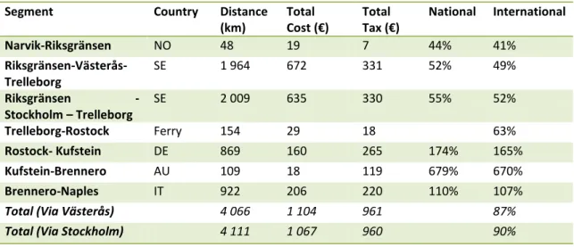
CO2 Total Fairway due Total Internali-sation ratio (Good) (GT) Oslo-Rotterdam North sea 1 028 50 969 6 546 57 515 0% Oslo-Gothenburg North sea 302 13 904 1 923 15 827 1 637 1 485 3 121 20% Oslo- Gothenburg – Rotterdam North sea 1 230 56 629 7 833 64 461 1 637 1 485 3 121 5% 5.2 Narvik – Naples Road
Table 17 presents the results of the road transport between Narvik and Naples. This segment contains two different routes through Sweden, one via Västerås and another via Stockholm. The main cost is wear and tear, followed by air pollution along the Oslo – Rotterdam corridor. The difference between the alternatives is mainly attributed to a higher share of motorways in Alternative 2, i.e. the Swedish segment, which generates a lower cost for wear and tear as well as accidents. In this corridor, the external costs per vehicle kilometre vary more greatly than in the Oslo – Rotterdam corridor, especially for the Northern parts i.e. Norway and Sweden. This result is mainly due to the high share of non-motorways in these segments.