DISSERTATION
ADVANCES IN STATISTICAL ANALYSIS AND MODELING OF EXTREME VALUES MOTIVATED BY ATMOSPHERIC MODELS AND DATA PRODUCTS
Submitted by Miranda J. Fix Department of Statistics
In partial fulfillment of the requirements For the Degree of Doctor of Philosophy
Colorado State University Fort Collins, Colorado
Fall 2018
Doctoral Committee: Advisor: Daniel Cooley Jennifer Hoeting Ander Wilson Elizabeth Barnes
Copyright by Miranda J. Fix 2018 All Rights Reserved
ABSTRACT
ADVANCES IN STATISTICAL ANALYSIS AND MODELING OF EXTREME VALUES MOTIVATED BY ATMOSPHERIC MODELS AND DATA PRODUCTS
This dissertation presents applied and methodological advances in the statistical analysis and modeling of extreme values. We detail three studies motivated by the types of data found in the atmospheric sciences, such as deterministic model output and observational products. The first two investigations represent novel applications and extensions of extremes methodology to climate and atmospheric studies. The third investigation proposes a new model for areal extremes and develops methods for estimation and inference from the proposed model.
We first detail a study which leverages two initial condition ensembles of a global climate model to compare future precipitation extremes under two climate change scenarios. We fit non-stationary generalized extreme value (GEV) models to annual maximum daily precipita-tion output and compare impacts under the RCP8.5 and RCP4.5 scenarios. A methodological contribution of this work is to demonstrate the potential of a “pattern scaling” approach for extremes, in which we produce predictive GEV distributions of annual precipitation maxima under RCP4.5 given only global mean temperatures for this scenario. We compare results from this less computationally intensive method to those obtained from our GEV model fitted di-rectly to the RCP4.5 output and find that pattern scaling produces reasonable projections.
The second study examines, for the first time, the capability of an atmospheric chemistry model to reproduce observed meteorological sensitivities of high and extreme surface ozone (O3). This work develops a novel framework in which we make three types of comparisons be-tween simulated and observational data, comparing (1) tails of the O3response variable, (2) dis-tributions of meteorological predictor variables, and (3) sensitivities of high and extreme O3to meteorological predictors. This last comparison is made using quantile regression and a recent tail dependence optimization approach. Across all three study locations, we find substantial
differences between simulations and observational data in both meteorology and meteorolog-ical sensitivities of high and extreme O3.
The final study is motivated by the prevalence of large gridded data products in the atmo-spheric sciences, and presents methodological advances in the (finite-dimensional) spatial set-ting. Existing models for spatial extremes, such as max-stable process models, tend to be geo-statistical in nature as well as very computationally intensive. Instead, we propose a new model for extremes of areal data, with a common-scale extension, that is inspired by the simultane-ous autoregressive (SAR) model in classical spatial statistics. The proposed model extends re-cent work on transformed-linear operations applied to regularly varying random vectors, and is unique among extremes models in being directly analogous to a classical linear model. We specify a sufficient condition on the spatial dependence parameter such that our extreme SAR model has desirable properties. We also describe the limiting angular measure, which is dis-crete, and corresponding tail pairwise dependence matrix (TPDM) for the model.
After examining model properties, we then investigate two approaches to estimation and inference for the common-scale extreme SAR model. First, we consider a censored likelihood approach, implemented using Bayesian MCMC with a data augmentation step, but find that this approach is not robust to model misspecification. As an alternative, we develop a novel estimation method that minimizes the discrepancy between the TPDM for the fitted model and the estimated TPDM, and find that it is able to produce reasonable estimates of extremal dependence even in the case of model misspecification.
ACKNOWLEDGEMENTS
I would not be here without the guidance and steadfast support of my advisor, Dan Cooley. Dan has been a great role model, both as a patient teacher and mentor, and as a researcher with vision and perspective. Our meetings often gave me a renewed sense of purpose and direction. I am grateful to Dan for exposing me to the broader extremes community by funding and en-couraging me to attend international conferences and workshops. I feel very lucky to have had the opportunity to learn from and share ideas with many experts in the field.
A cornerstone of my graduate school experience was collaborating with world-class scien-tists at the National Center for Atmospheric Research (NCAR). Many thanks are due to Steve Sain, Claudia Tebaldi, and Brian O’Neill for including me in the BRACE project that kickstarted my research into climate extremes. I also learned a great deal from analyzing ozone extremes in collaboration with Alma Hodzic and Eric Gilleland. In addition, I am grateful to Doug Nychka and Dorit Hammerling for treating me like family.
I owe many thanks to Emeric Thibaud for his assistance on the extreme SAR project. Emeric is not only a brilliant researcher, but also a wonderfully kind mentor, and I appreciated our brainstorming sessions. I am also grateful to Ben Shaby for taking the time to chat about MCMC, and to Raphaël Huser for a memorable conversation in the Swiss Alps. Thanks also to Brook Russell and Will Porter for paving the way on the ozone project.
Colorado State University has been an incredibly supportive community. I would like to thank my committee members Jennifer Hoeting, Ander Wilson, and Libby Barnes, for their helpful feedback. Though she may not know it, Jennifer was one of the reasons I decided to come to CSU, and I am so grateful to her for believing in me. I would also like to thank Phil Turk for being another advocate as well as my mentor in the realm of statistical consulting. I send heartfelt thanks to Kristina Quynn and the rest of CSU Writes for helping me rediscover the joy and pleasure of writing. Additionally, none of this could have happened without excellent administrative assistance from Kristin Stephens and Katy Jackson.
I was fortunate to receive funding from many sources during my time at CSU, including CSU’s Center for Interdisciplinary Mathematics and Statistics fellowship, Environmental Pro-tection Agency grant EPA-STAR RD-83522801-0, and National Science Foundation grant DMS-1243102. Additional travel funding was provided by the Research Network for Statistical Meth-ods for Atmospheric and Oceanic Sciences (STATMOS).
I have had the great fortune to get to know an amazing group of graduate students and post-docs who have inspired and supported me throughout the past five years. Special thanks to Josh Hewitt, Clint Leach, Erin Gorsich, Magda Garbowski, and Henry Scharf for all the times they showed up to write, chat, or toss a disc. Special thanks to the Tomato Club for helping me persevere. Thanks also to my roommate Morgan Hawker and my pseudo-roommate Jessica Mao for their warmth and generosity.
The Fort Collins ultimate community was instrumental in keeping me active and sane. I must also thank the wonderful physical therapists and fitness professionals, including Katie Hall, Bryan Duran, Sue Rutherford, Eric Maxwell, and Kelly Buell-Schoenman, who have helped me move more easily through the world.
No acknowledgements section would be complete without recognizing the fundamental support from my family. I would like to thank my parents, Charlotte Lo and Douglas Fix, for motivating me to pursue a PhD in the first place, and for their unwavering confidence in my ability to do whatever I set my mind to. Finally, I am immeasurably grateful to my partner, David Betz, for being my cheerleader and my rock. You have the biggest heart and inspire me to be better every day. Thanks for waiting.
DEDICATION
TABLE OF CONTENTS ABSTRACT . . . ii ACKNOWLEDGEMENTS . . . iv DEDICATION . . . vi LIST OF TABLES . . . ix LIST OF FIGURES . . . x Chapter 1 Introduction . . . 1 1.1 Motivation . . . 1 1.2 Outline . . . 2 1.3 Univariate Extremes . . . 4
1.3.1 Block maxima approach . . . 4
1.3.2 Threshold exceedance approach . . . 7
1.4 Multivariate Extremes and Regular Variation . . . 8
1.4.1 Asymptotic theory of multivariate regular variation . . . 10
1.4.2 Link to multivariate extreme value distributions . . . 13
1.4.3 Statistical inference for multivariate extremes . . . 14
1.5 Process Setting . . . 16
1.5.1 Asymptotic theory . . . 16
1.5.2 Statistical inference for spatial extremes . . . 18
Chapter 2 A Comparison of US Precipitation Extremes Under RCP8.5 and RCP4.5 with an Application of Pattern Scaling . . . 19
2.1 Introduction . . . 19
2.2 Methods . . . 22
2.2.1 Output from initial condition ensembles . . . 22
2.2.2 GEV modeling conditional on global mean temperature . . . 23
2.2.3 Pattern scaling . . . 25
2.3 Results . . . 26
2.3.1 Estimates for CESM-LE (historical/RCP8.5) . . . 26
2.3.2 Comparison with CESM-ME (RCP4.5) . . . 27
2.3.3 Results of pattern scaling . . . 30
2.3.4 Ensemble advantage for shape parameter estimation . . . 31
2.4 Discussion . . . 33
Chapter 3 Observed and Predicted Sensitivities of High and Extreme Surface Ozone to Meteorological Drivers in Three US Cities . . . 36
3.1 Introduction . . . 36
3.2 Inputs . . . 39
3.2.1 Observations and NARR . . . 39
3.2.2 NRCM-Chem simulations . . . 40
3.3 Statistical Methods . . . 42
3.3.1 Marginal analysis of extreme O3 . . . 42
3.3.2 Relating high and extreme O3to meteorological drivers . . . 44
3.4 Results . . . 47
3.4.1 Comparing tails of O3response . . . 47
3.4.2 Comparing meteorological predictors . . . 48
3.4.3 Comparing relationships between O3and meteorology . . . 50
3.5 Summary and Discussion . . . 53
Chapter 4 Simultaneous Autoregressive Models for Spatial Extremes . . . 57
4.1 Introduction . . . 57
4.2 Background . . . 58
4.2.1 Classical SAR model . . . 58
4.2.2 Transformed-linear operations on regularly varying random vectors . . 60
4.3 Extreme SAR Models . . . 65
4.3.1 A SAR-inspired model for areal extremes . . . 65
4.3.2 An extreme SAR model with common scale . . . 70
4.4 Discussion . . . 71
Chapter 5 Estimation and Inference for Extreme SAR Models . . . 74
5.1 Introduction . . . 74
5.2 Data . . . 75
5.2.1 Simulation from the true model . . . 76
5.2.2 Simulation from a Brown-Resnick process . . . 76
5.2.3 Gridded precipitation observations . . . 81
5.3 Censored Likelihood with Bayesian Data Augmentation . . . 82
5.3.1 Methods . . . 82
5.3.2 Results . . . 88
5.4 Fitting via the TPDM . . . 91
5.4.1 Methods . . . 91
5.4.2 Results . . . 94
5.5 Discussion . . . 106
Chapter 6 Conclusions and Future Work . . . 109
References . . . 112
LIST OF TABLES
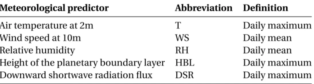
3.1 Meteorological predictors and corresponding daily summary measures . . . 41 3.2 GPD parameter estimates for simulated and observed summer MDA8 O3 . . . 48 5.1 Results from a censored likelihood approach with Bayesian data augmentation . . . . 88 5.2 Results from fitting via the TPDM for data simulated from the true model . . . 100 5.3 Results from fitting via the TPDM for Brown-Resnick simulations . . . 104
LIST OF FIGURES
1.1 Illustration of the three extremal types . . . 6
1.2 Illustration of the directionality of risk . . . 11
1.3 Illustration of two definitions for multivariate threshold exceedances . . . 14
2.1 Comparison of observed and simulated annual maximum daily precipitation . . . 21
2.2 Results for CESM-LE under RCP8.5 . . . 28
2.3 Comparison of 1% AEP levels under RCP4.5 and RCP8.5 . . . 29
2.4 Evaluation of pattern scaling precipitation extremes . . . 31
2.5 Demonstration of ensemble advantage for shape parameter estimation . . . 32
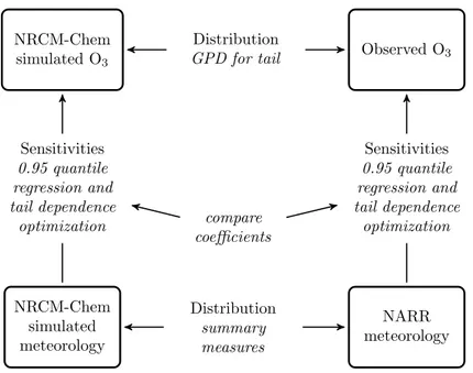
3.1 Illustration of study framework . . . 39
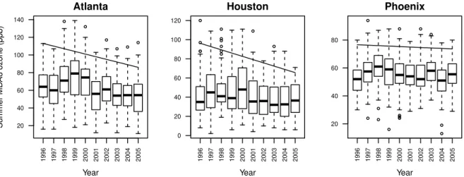
3.2 Distribution of observed summer MDA8 O3by year at three AQS stations. . . 43
3.3 Boxplots of summer MDA8 O3from NRCM-Chem simulations and AQS observations 47 3.4 Kernel density plots of NRCM-Chem and NARR meteorological variables . . . 49
3.5 Coefficient plots for 0.95 quantile regression and tail dependence optimization . . . . 51
4.1 Two common neighborhood definitions for the classical SAR model . . . 59
4.2 Specific transform used for transformed-linear operations . . . 61
4.3 Illustration of how the extremal SAR model induces spatial dependence . . . 69
4.4 Tail pairwise dependence matrices for two extremal SAR models . . . 70
5.1 Pairwise extremal dependence measures: Brown-Resnick vs. true extreme SAR model 80 5.2 Example of gridded precipitation data before and after marginal transformation . . . 82
5.3 Example MCMC diagnostic plots for theρ parameter chain for data simulated from the true model . . . 89
5.4 Illustration of y sampling for data simulated from the true model . . . 90
5.5 Issues with the censored likelihood approach applied to Brown-Resnick simulations 91 5.6 Comparison of two estimators of ΣYfor data simulated from the true model . . . 95
5.7 Illustration of the proposed approach to bias correction of ˆΣY . . . 96
5.8 Effect of threshold selection on estimates ofρ from extreme SAR simulations . . . 99
5.9 Comparison of two estimators of ΣYfor a Brown-Resnick simulation . . . 101
5.10 Illustration of bias correction of ˆΣYfor a Brown-Resnick simulation . . . 101
5.11 Comparison of ΣY( ˆρ) and ΣB Rfor a Brown-Resnick simulation . . . 102
5.12 Effect of threshold selection on estimates ofρ from Brown-Resnick simulations . . . 104
5.13 Results from fitting via the TPDM for gridded precipitation observations . . . 105
A.1 GEV parameter estimates for CESM-LE under RCP8.5 . . . 126
A.2 P-values associated with one-sided hypothesis tests ofµ8.51 (s) ≤ 0 and φ8.51 (s) ≤ 0 . . . 127
A.3 Anderson-Darling goodness of fit results for the GEV model (CESM-LE) . . . 127
A.4 Estimated standard errors for 1% AEP levels under RCP8.5 . . . 127
A.5 GEV parameter estimates for CESM-ME under RCP4.5 . . . 128
A.6 P-values testingµ4.51 (s) ≤ 0 and φ4.51 ≤ 0, and a comparison of µ4.51 (s) andµ8.51 (s) . . . . 129
A.8 Estimated 1% AEP levels for CESM-ME under RCP4.5 . . . 130 A.9 Difference in the year 2080 between pattern-scaled and CESM-ME projections . . . . 130
Chapter 1
Introduction
1.1 Motivation
In September 2013, Colorado experienced its second most costly natural disaster (Lukas et al., 2014). Severe flooding inundated the Front Range during one of the region’s most ex-treme rainfall events on record. In total, there were eight flood-related fatalities and damages exceeded $2 billion (Gochis et al., 2015). This flooding event, and others like it, are extreme events. Such events occur infrequently but can impose a high cost on society. Extreme value theory (EVT) was developed in the early part of the 20th century to understand the asymptotic distribution of the largest order statistic. Development of statistical methodology for extreme events was spurred by the devastating North Sea flood of 1953 that killed more than 1800 people in the Netherlands, and statistical analyses contributed to decision making about the height of the Dutch dykes (de Haan, 1990). While the earliest applications of EVT focused primarily on hydrology and civil engineering, these days the need to characterize the likelihood and severity of extreme events applies to a wide variety of fields, including atmospheric science, finance, telecommunications, forest fire science, and public health.
This dissertation presents applied and methodological advances in the analysis of extreme values. The main goal of an extreme value analysis is to describe the upper (or lower) tail of a probability distribution. In the univariate case, the aim is to characterize the tail of the distribu-tion of a single variable, such as daily precipitadistribu-tion at a weather stadistribu-tion. A multivariate analysis may consider the joint tail (i.e., the tail dependence structure) of several variables, such as daily ozone levels and air temperature at a certain location, or, in the spatial setting, a single variable measured at several neighboring locations. Traditional statistical methods that aim to describe the bulk of a distribution, and may employ such summary measures as means, variances or correlations, are not useful for describing the tail. Because the focus is on the tail, extreme value analyses typically use only the extreme observations, discarding the bulk of the data. By
definition, extremes are rare, so in the study of extremes we are always data poor. Moreover, extreme value analyses often require estimating the probability of events that are more extreme than any that have previously been observed. EVT provides a theoretical framework for such extrapolations, with extreme value models generated by asymptotic arguments.
The work in this dissertation is largely motivated by the types of data found in the atmo-spheric sciences. We consider large ensembles of global climate model output (Chapter 2), compare high resolution atmospheric chemistry model output to station observations and re-analysis (Chapter 3), and propose a new model and develop new inference methods for areal extremes motivated by the prevalence of atmospheric datasets that are indexed by regular grids (Chapter 4 and Chapter 5).
1.2 Outline
The remainder of this chapter (Chapter 1) provides an overview of EVT concepts essential to this dissertation. We first briefly review classical univariate EVT, including block maxima and threshold exceedance approaches. We then introduce the framework of multivariate regular variation and tie it back to multivariate extreme value distributions. We end with a few notes on extremes in the (spatial) process setting. Our review is far from exhaustive, thus we point the reader to several excellent books on the probability theory underlying the study of extremes, including Resnick (1987) and de Haan and Ferreira (2006), as well as the statistical analysis of extremes, such as Coles (2001) and Beirlant et al. (2006).
Chapter 2 leverages two initial condition ensembles of a global climate model to compare future precipitation extremes under two climate change scenarios. A methodological contribu-tion of this work is to demonstrate the potential of a “pattern scaling" approach for extremes. This chapter is based on an article published in Climatic Change.1
1Fix, M. J., Cooley, D., Sain, S. R., & Tebaldi, C. (2018). A comparison of US precipitation extremes under RCP8.5
Chapter 3 considers the complex question of how to evaluate the ability of a high resolution atmospheric chemistry model to reproduce observed relationships between meteorology and high or extreme surface ozone. A contribution of this work is to develop a novel framework for comparing simulations and observational data products. We uniquely investigate meteorologi-cal sensitivities, extending a recent approach relating extreme responses to a set of atmospheric drivers. This chapter is based on an article published in Atmospheric Environment.2
Chapter 4 is motivated by the preponderance of large gridded products in the atmospheric sciences. Existing models for spatial extremes, such as max-stable process models, tend to be geostatistical in nature as well as very computationally intensive. The goal of this work is to develop a simple spatial extremes model that is computationally feasible for high-dimensional areal data. To this end, Chapter 4 proposes extremal versions of the classical simultaneous au-toregressive (SAR) model. Linear models are ubiquitous in traditional (non-extreme) statistics, but to our knowledge this is the first extremes model that is directly analogous to a classical lin-ear model. One property of our extreme SAR model is that its limiting angular measure, which characterizes the tail dependence structure, is discrete in nature. Similar extremal models have been found to be challenging for inference. Chapter 4 also describes the tail pairwise depen-dence matrix (TPDM) which summarizes this dependepen-dence.
Building upon Chapter 4, Chapter 5 presents several approaches to estimation and infer-ence for the extreme SAR model, and discusses their respective challenges. We investigate a Bayesian approach, which relies on a likelihood specification. Likelihood approaches for ex-tremes models with discrete dependence structure have not been previously investigated. We also develop a novel estimation method that minimizes the discrepancy between the TPDM for the fitted model and the estimated TPDM, and find that it is able to produce reasonable dependence estimates even in the case of model misspecification.
2Fix, M. J., Cooley, D., Hodzic, A., Gilleland, E., Russell, B. T., Porter, W. C., & Pfister, G. G. (2018). Observed and
predicted sensitivities of extreme surface ozone to meteorological drivers in three US cities. Atmospheric
Finally, Chapter 6 concludes the dissertation with a brief summary of the work completed and remarks on future extensions of each of the projects.
1.3 Univariate Extremes
1.3.1 Block maxima approach
Asymptotic theoryClassical extreme value models arise from arguments regarding the limiting distribution of suitably renormalized block maxima. Let X1, . . . , Xnrepresent independent copies of a random variable X with common (“parent") distribution function F . Consider Mn= max(X1, . . . , Xn), and note that P(Mn≤ x) = Fn(x). For F (x) < 1, Fn(x) → 0 as n → ∞, so Fn(x) converges to a degenerate distribution function with a point mass at the upper endpoint sup{x : F (x) < 1}. Instead, we consider limiting distributions of renormalized maxima Mn−bn
an , for appropriate
choices of an > 0 and bn ∈ R. The Extremal Types Theorem, first introduced by Fisher and Tippett (1928) and later rigorously proven by Gnedeko (1943), provides a fundamental result. If there exist sequences of constants an> 0 and bnsuch that, as n → ∞,
P µ Mn− bn an ≤ x ¶ = Fn(anx + bn) → G(x) (1.1)
for some non-degenerate distribution function G, then G must belong to one of the following types of extreme value distributions:
Type I (Gumbel): G(x) = exp{−exp(−x)} , x ∈ R (1.2)
Type II (Fréchet): G(x) = 0, x ≤ 0, exp(−x−α), x > 0 (1.3)
Type III (reverse Weibull): G(x) = exp(−(−x)α), x < 0, 1, x ≥ 0 (1.4)
for someα > 0. This result is powerful because when the limiting distribution G exists, it follows one of the above distributions irrespective of the parent distribution F . We say F is in the domain of attraction (MDA) of G. The extreme value distributions are equivalent to the max-stable distributions, defined as the distributions for which there exist sequences an > 0 and bn∈ R such that Gn(anx + bn) = G(x) for all positive integers n and all x ∈ R.
The three extremal types above can be combined into a single parametric family known as the generalized extreme value (GEV) distribution with the form
G(x) = exp ½ − h 1 + ξ³ x −µ σ ´i−1/ξ + ¾ , (1.5)
whereµ ∈ R is the location parameter, σ > 0 is the scale parameter, ξ ∈ R is the shape parameter, and y+:= max(y,0). The support of G is {x ∈ R : 1+ξ(x −µ)/σ > 0}. The shape parameter ξ deter-mines the tail behavior (see Figure 1.1). Ifξ = 0 (we take the limit of (1.5) as ξ → 0), then the tail is light and G is Gumbel. The Gamma and Gaussian distributions are examples of distributions that are in the MDA of G withξ = 0. If ξ > 0, then the tail is heavy and G is Fréchet. The Student t distribution is in the MDA of G withξ =d . f .1 > 0. If ξ < 0, then the upper tail is bounded and G is reverse Weibull. The Beta distribution is in the MDA of G withξ < 0.
Statistical inference
In practice, the limit in (1.1) is interpreted as an approximation for large n, and the GEV family can be used for modeling the distribution of block (e.g., annual or seasonal) maxima. We do not need to estimate the renormalizing sequences anand bnbecause they can be absorbed into theµ and σ parameters of the GEV (Coles, 2001). Suppose one begins with iid data xb,i in-dexed by block b = 1,...,B and time-within-block i = 1,...,n. Letting mn,b= maxi =1,...,nxb,i, one obtains B block maxima from which the parameters of the GEV distribution can be estimated
−4 −2 0 2 4 0.0 0.2 0.4 0.6 0.8 1.0 x density
Figure 1.1: Illustration of the three extremal types: standard Gumbel (black), unit Fréchet (blue), and unit reverse Weibull (red) density functions.
via maximum likelihood (Prescott and Walden, 1980; Smith, 1985) or moment-based methods like probability-weighted moments (Hosking et al., 1985). From the fitted model, we can obtain estimates of high quantiles (so-called “return levels" in environmental science) along with the associated uncertainties.
The extreme value distributions can be thought of as “ultimate" approximations that hold in the limit, i.e., as block size n goes to infinity. In practice, accuracy may be increased by us-ing a penultimate approximation to the distribution of Mnfor finite n (Embrechts et al., 2012; Katz, 2013). This was noted as early as Fisher and Tippett (1928), who showed that takingξ < 0 (reverse Weibull type) provides a better approximation for maxima of finite samples from the Gaussian distribution than does the limiting Gumbel distribution. This means that there is no advantage to constraining the estimation procedure toξ = 0 even if the correct limiting distri-bution is known to be Gumbel (Furrer and Katz, 2008).
1.3.2 Threshold exceedance approach
Asymptotic theoryA disadvantage of the block maxima approach is that it may be wasteful of data. Although many extreme events could have occurred in the same block, only one event per block is re-tained and the rest discarded. An alternative is to fix a high threshold u and retain all observa-tions above this threshold. The classical asymptotically motivated model for exceedances over a high threshold is the generalized Pareto distribution (GPD). Suppose F is in the MDA of a GEV distribution G. Then for large enough u, the distribution function of threshold excesses is approximately given by the GPD:
P(X − u ≤ x | X > u) ≈ 1 − µ 1 +ξx σu ¶−1/ξ + , (1.6)
where ξ is equivalent to the shape parameter of the GEV distribution and σu = σ + ξ(u − µ) (Balkema and de Haan, 1974; Pickands, 1975). In the case ξ → 0, the right-hand side of (1.6) becomes 1 − exp(−x/σu).
Below we outline a justification for the GPD from Coles (2001). Assume X , X1, X2, . . . ,i i d∼ F and F ∈ MDA(G). Then for large enough n, following from (1.1) we have the approximation
n log F (x) ≈ −h1 + ξ³ x −µ σ
´i−1/ξ
+ . (1.7)
For large values of x, a Taylor expansion gives log F (x) ≈ −[1 − F (x)]. Hence for large u,
1 − F (u) ≈ n−1h1 + ξ³u −µ σ
´i−1/ξ
+ , (1.8)
and similarly for x > 0,
1 − F (u + x) ≈ n−1h1 + ξ³u +x −µ σ
´i−1/ξ
+ . (1.9)
P(X > u + x|X > u) =1 − F (u + x) 1 − F (u) =n −1£1 + ξ¡u+x−µ σ ¢¤−1/ξ + n−1£1 + ξ¡u−µ σ ¢¤−1/ξ + = µ 1 +ξx σu ¶−1/ξ + , (1.10)
whereσu= σ + ξ(u − µ) and (1.10) is the survival function of the GPD.
Statistical Inference
The result (1.6) suggests a framework for statistical modeling of threshold exceedances. Starting with the original data x1, . . . , xN, extreme events can be identified by selecting a high threshold u above which the distribution’s tail is well approximated by a GPD. The observations that exceed u, i.e., {xi : xi > u}, can be labeled x(1), . . . , x(Nu), where Nu is the number of
ex-ceedances. Then the threshold excesses yj = x( j )− u, j = 1,..., Nu, can be used to estimate the parametersσuandξ by either numerical maximum likelihood or moment-based approaches.
Statistical application of the GPD requires the choice of a suitable threshold, which involves a bias-variance tradeoff. The threshold must be sufficiently high for the GPD to be an appro-priate model for the tail. On the other hand, raising the threshold reduces the sample size and thus increases the variance of the parameter estimates. In practice there are several diagnostic aids for threshold selection. Scarrott and MacDonald (2012) provide a review of some of the existing approaches. The penultimate approximation described in Section 1.3.1 for the GEV distribution applies equally well to the corresponding GPD (Furrer and Katz, 2008).
1.4 Multivariate Extremes and Regular Variation
There are several related approaches for modeling multivariate extremes. The classical ap-proach is based on the multivariate extreme value distributions (MVEVDs; see Section 1.4.2). These arise as the limiting distributions of suitably normalized componentwise maxima and can be developed in a multivariate analogue to the argument leading to the Extremal Types
Theorem and the GEV distribution (de Haan and Ferreira, 2006, Sections 6.1 and 6.2). As such, MVEVDs provide sensible models for componentwise sample maxima. Note that componen-twise maxima are not an entirely intuitive concept, as maxima in different components can occur at different times.
Akin to univariate extremes, threshold exceedance approaches can also be taken for mod-eling multivariate extremes. Such approaches require defining what is meant by a multivariate threshold exceedance. The multivariate GPD of Rootzén and Tajvidi (1997) can be used when thresholds are defined in terms of each univariate marginal, i.e., extreme events are described in terms of Cartesian coordinates. The probabilistic framework of multivariate regular variation (MVRV; see Section 1.4.1) is well-suited for defining a threshold in terms of a vector norm, and is easily described in terms of pseudo-polar coordinates.
The above approaches to multivariate extreme value modeling share several commonal-ities. In all cases, there is no finite parameterization for the class of dependence structures (but parametric models may be specified). For each approach, characterization of the depen-dence structure is made easier by imposing assumptions on the marginal behavior, and conse-quently estimation of the dependence structure from data often requires transformation of the marginals. As in the univariate case, models for multivariate extremes are fit only to observa-tions deemed extreme. The approaches are also theoretically linked, as each can be tied to the so-called angular measure, which we will describe in more detail in Section 1.4.1. This angular measure fully characterizes dependence in the limit.
Within this dissertation, we will focus on the MVRV framework for modeling multivariate threshold exceedances. MVRV provides a probabilistic characterization of the joint (upper) tail of a random vector, and is defined entirely in terms of the joint tail. The MVRV framework assumes the heavy-tailed case, i.e., it implies that the joint tail decays like a power function. MVRV is most easily understood via a pseudo-polar decomposition. The limiting angular mea-sure mentioned above arises from this decomposition. Below we provide definitions and
back-ground on MVRV (Section 1.4.1), explain its connection to MVEVDs for componentwise max-ima (Section 1.4.2), and discuss methods of inference (Section 1.4.3).
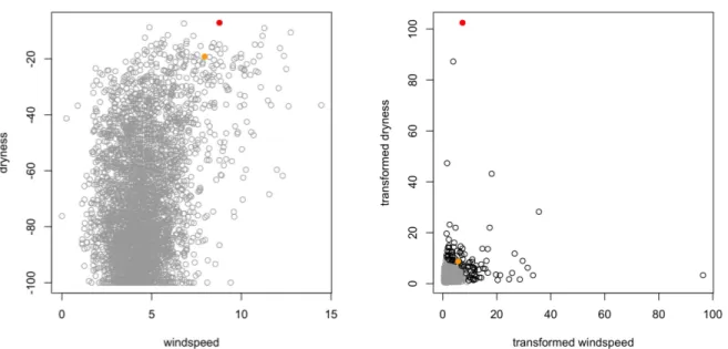
Although MVRV can be defined on Rp (Resnick, 2007, Section 6.5.5), we model in the non-negative orthant to focus attention on the upper tail. In applications, there is often a natural di-rection in which one wants to assess risk. Consider wildfire risk, which is related to many factors including fuel and weather conditions. For example, high windspeed and low humidity (high dryness) are associated with increased fire risk. The left panel of Figure 1.2 shows daily sum-mary measures for windspeed and dryness at a weather station in southern California. More details about these data can be found in Cooley et al. (2018). Wildfires, such as those indicated by the colored points, tend to occur in the upper right, when both variables are high. Thus this is the direction of interest. Note that the raw data are not regularly varying, so for a MVRV analy-sis it is necessary to perform a marginal transformation as discussed earlier. As an example, the right panel of Figure 1.2 shows the same data after transformation to Fréchet(α = 2) marginals. With the transformed data, one could use the MVRV on the nonnegative orthant to model the tail dependence between the daily windspeed and dryness variables, and ultimately estimate the probabilities associated with risk regions where both variables are high.
1.4.1 Asymptotic theory of multivariate regular variation
Resnick (2007) presents several equivalent definitions of MVRV, including the following. Let Z be a random vector taking values in the nonnegative orthant Rd+= [0,∞)d. Let M+(C) denote
the space of nonnegative Radon measures onC= [0,∞]d\ {0}. We say Z is regularly varying if
there exists a sequence cn→ ∞ and a limit measure ν(·) on the Borel subsets of Rd+such that
nP µZ cn ∈ · ¶ v → ν(·) (1.11)
in M+(C) as n → ∞, where→ denotes vague convergence of measures. One recognizes fromv
defini-Figure 1.2: Illustration of the directionality of risk: wildfire example. Left: daily summary measures of windspeed and dryness at a weather station in southern California during the years 1973-2015. Right:
Transformed data with Fréchet(α = 2) marginals. Black circles indicate observations exceeding the 0.975
quantile of the radial component (L2norm). In both panels, orange and red points correspond to the
initial days of two of the most destructive wildfires during the observation period.
tions of MVRV in terms of counting measures converging to a Poisson random measure with mean measureν (Resnick, 2007, Section 6.2).
The limit measureν can be shown to have the scaling property
ν(p A) = p−αν(A) (1.12)
for any set A ⊂Cand any p > 0, where α > 0 is termed the tail index and determines the
power-law behavior of the tail. We denote a d -dimensional regularly varying random vector Z with tail indexα by Z ∈ RV+d(α).
The scaling property (1.12) suggests a transformation to pseudo-polar coordinates, and leads to an equivalent definition of MVRV. Given any norm || · ||, denote the nonnegative unit sphere Sd −1+ =©z ∈ Rd+: ||z|| = 1ª. We define “radial" and “angular" components by R = ||Z|| and Θ= ||Z||−1Z, respectively. Then the random vector Z is regular varying if there exists a sequence cn→ ∞ and a finite measure H on Sd −1+ such that for any H -continuity Borel set B ⊂ Sd −1+ , and for r > 0,
nP µ R cn > r,Θ ∈ B ¶ v → r−αH (B ) (1.13)
as n → ∞. The right-hand side of (1.13) is a product measure, indicating that the radial and an-gular components become independent in the limit. H is termed the anan-gular measure (some-times also referred to as the spectral measure), and completely characterizes the limiting tail dependence structure of Z. The normalizing sequence {cn} can be chosen such that H is a prob-ability measure, although in many modeling situations it may make sense for H to have total mass other than one. It is often assumed that Z has common marginal distributions, which imposes the following balance condition on H (Resnick, 1987):
Z Sd −1 + θ1H (d θ) = Z Sd −1 + θjH (d θ), j = 2,...,d. (1.14)
To provide some intuition on the angular measure, consider the bivariate case Z = (Z1, Z2)⊤∈ RV+2(α) with common marginal distributions. There are two limiting cases. If Z exhibits perfect dependence, i.e., if Z1determines Z2exactly, then H consists of a single point mass on the in-terior of S1+. In the asymptotic independence case, i.e., if limz→∞P(Z2> z|Z1> z) = 0, then H consists of two point masses, one at each end of the one-dimensional unit sphere. In general, dependence increases as the mass of H concentrates toward the center of Sd −1+ and decreases as it moves towards the edges and vertices of Sd −1+ .
Although the polar-coordinate geometry is natural for describing regular variation, it can be hard to reconcile with the Cartesian geometry required by cumulative distribution functions and other familiar notions. Geometric arguments can give needed expressions. For a given norm || · ||, tail index α, and angular measure H, consider the set A = [0,z]c
for z = (z1, . . . , zd)⊤∈ C. Then ν(A) = Z A αr−α−1d r d H (θ) = Z Sd −1 + Z∞ r =Vdi =1ziθi αr−α−1d r d H (θ)
= Z Sd −1 + d _ i =1 µ zi θi ¶−α H (d θ). (1.15)
1.4.2 Link to multivariate extreme value distributions
Analogous to the univariate block maxima approach described in Section 1.3.1, classical multivariate EVT considers the limiting distribution of the vector of appropriately renormal-ized componentwise maxima. Let X = (X1, . . . , Xd)⊤ be a d -dimensional random vector with marginals F1, . . . , Fd and joint distribution F . Suppose we have n iid replicate vectors {Xi}ni =1 and define the vector of componentwise maxima Mn=¡Wni =1Xi ,1, . . . ,Wni =1Xi ,d
¢⊤
. Note that Mn does not necessarily correspond to an observed data point, as maxima may not occur at the same time in each margin. If there exist renormalizing sequences of vectors an≥ 0 and bn∈ Rd such that P µ Mn− bn an ≤ z ¶ = Fn(anz + bn) → G(z) (1.16)
(non-degenerate) as n → ∞, where all operations are componentwise, then G is a multivariate extreme value distribution (MVEVD). A sequence of random vectors can only converge if all the marginals converge, so Fjn(anz + bn) → Gj(z) for j = 1,...,d. Thus G has univariate GEV marginals. Although the marginals are fully parameterized, no finite parameterization exists for the dependence structure of the d components.
The MVRV framework can be tied back to classical multivariate EVT, in that MVRV is a con-dition implying that a distribution is in the MDA of a MVEVD (Beirlant et al., 2006; Resnick, 1987). Let Z ∈ RV+d(α) with limit measure ν as in (1.11), and let Mnbe the vector of componen-twise maxima of n iid realizations of Z. Then there exist renormalizing sequences of vectors an≥ 0 and bn∈ Rd such that (1.16) holds with G(z) = exp{−ν[0,z]c}, and the marginals of G are GEV withξ = 1/α > 0. In other words, Z is in the MDA of a MVEVD with Fréchet(α) margins and dependence structure characterized by the measureν from (1.15).
1.4.3 Statistical inference for multivariate extremes
The classical approach to statistical inference for multivariate extremes consists of parti-tioning a sample of multivariate observations into blocks and fitting a MVEVD to the sample of componentwise block maxima. Beirlant et al. (2006) describes both parametric and nonpara-metric techniques to estimate the MVEVD dependence structure. More efficient inference can be performed using threshold methods, and in this dissertation we focus on statistical inference for multivariate threshold exceedances within the MVRV framework. There are several possible approaches to define a threshold exceedance in the multivariate setting. Here we consider two definitions, one in terms of the norm of a random vector, and one in terms of the marginals, as illustrated in Figure 1.3. In the first case, an exceedance is defined as an observation whose norm (radial component) exceeds a suitably high threshold. In the second case, a multivariate observation is considered an exceedance if at least one of its components exceeds its marginal threshold. 0 50 100 150 200 0 50 100 150 200 z1 z2 0 50 100 150 200 0 50 100 150 200 z1 z2
Figure 1.3: Illustration of two definitions for multivariate threshold exceedances, for d = 2 and with unit Fréchet margins. Colored points are exceedances, and dotted lines indicate the norm threshold (left) or marginal thresholds (right). On the right, blue points are those which exceed the marginal threshold in only one component; these observations would be censored under a censored likelihood approach.
The MVRV framework implies that the marginal distributions are univariate regularly vary-ing with common tail indexα. In statistical practice, a standard approach is to transform the univariate marginals to a convenient distribution with commonα. This can be done by first estimating the marginal distributions, either parametrically or nonparametrically, and then ap-plying the probability integral transform. Doing so retains the tail dependence structure, as Proposition 5.10 of Resnick (1987) shows the MDA is preserved under monotone transforma-tions of the marginals. This approach is similar in spirit to a copula, but aims only to describe the tail.
After estimating the marginal effects, it is possible to focus on estimating the tail depen-dence structure, which is the crux of inference for multivariate extremes. Below we describe two general approaches to likelihood inference, corresponding to two definitions of thresh-old exceedances. The first approach consists of fitting an angular measure model to norm ex-ceedances. Finite-sample estimation of the angular measure assumes that the limit (1.13) is an equality for r > r0, where r0is a sufficiently high threshold. Assume that H is continuously dif-ferentiable with Radon-Nikodym derivative h(θ; η), which is termed the angular density. Then, given a parametric model for the angular density (see, e.g., Ballani and Schlather, 2011; Coles and Tawn, 1991; Cooley et al., 2010), it is possible to write down the corresponding likelihood for the points z1, . . . , zN0 for which ||zi|| = ri> r0, which is given by a Poisson point process
ap-proximation: L(η; z1, . . . zn) = exp µ −r0 cn ¶(YN0 i =1 ¡ αri−α−1/cn ¢ h(θi; η) ) /N0! ∝ N0 Y i =1 h(θi; η). (1.17)
Parameters can then be estimated via numerical maximum likelihood.
Alternatively, when an observation is defined to be a threshold exceedance if at least one of its components exceeds its marginal threshold, a censored likelihood approach is often used, where the non-extreme components are censored at their marginal thresholds (Ledford and
Tawn, 1996; Smith et al., 1997). Censored likelihood approaches reduce the bias that may arise from non-applicability of the limiting model in regions where not all components are extreme (Huser et al., 2016). More details on inference via censored likelihood will be given in Chapter 5. Likelihood-based inference for multivariate extremes can be challenging in high dimen-sions. Moreover, some models may fail to yield densities. Non-likelihood approaches are par-ticularly useful for models whose angular measures consist of discrete point masses, as we will return to in Chapter 5. Recent examples include M -estimators based on the continuous ranked probability score (Yuen and Stoev, 2014) and the stable tail dependence function (Einmahl et al., 2016), both of which are related to the underlying multivariate cumulative distribution func-tion. However, to our knowledge, applications of these methods to spectrally discrete models have been restricted to low-dimensional examples.
1.5 Process Setting
Thus far, we have introduced EVT in a finite dimensional setting, i.e., extremes of random variables or vectors. The asymptotic arguments of Section 1.3 can be extended to the infinite dimensional setting, i.e., extremes of stochastic processes. Extremal processes have primarily been used to model spatial extremes. Such models are typically geostatistical in nature, and are also challenging to fit. In Chapters 4 and 5 we will introduce and fit a very different type of spatial model than the extremal process models discussed here. Our proposed model is finite-dimensional, so a process is not needed. This multivariate model is very simple and is best suited for areal data, e.g., data on a regular grid. Our point in briefly discussing extremal process models here is to serve as contrast to the model we propose. A more comprehensive overview of statistical modeling for spatial extremes can be found in Davison et al. (2012).
1.5.1 Asymptotic theory
The natural extension of the GEV is the class of max-stable processes, which, under mild conditions, are the only possible non-degenerate limits of rescaled pointwise maxima of iid
random processes (de Haan, 1984). Let S be a compact subset of Rp, typically representing the spatial region of interest. Consider a random process Y = {Y (s)}s∈S defined over S, with
contin-uous sample paths, and let Y1, Y2, . . . be independent replicates of Y . If there exist sequences of continuous functions {an(s)}s∈S > 0 and {bn(s)}s∈S such that the limiting process Z = {Z (s)}s∈S
defined by
maxi =1,...,nYi(s) − bn(s)
an(s) → Z (s), s ∈ S, n → ∞,
(1.18)
is non-degenerate, then Z must be a max-stable process (de Haan, 1984; de Haan and Ferreira, 2006). We say that Y is in the MDA of Z . The marginals of Z are GEV-distributed, and can be transformed to a convenient distribution. For the remainder of this section, we will restrict attention to the commonly used simple max-stable processes with unit Fréchet margins. For every set of sites s1, . . . , sd ∈ S,
P{Z (s1) ≤ z1, . . . , Z (sd ≤ zd} = exp{−V (z1, . . . , zd)} , z1, . . . , zd> 0, (1.19)
where the exponent measure function V satisfies V (kz1, . . . , kzd) = k−1V (z1, . . . , zd), k > 0 and V (∞,...,∞, z,∞,...,∞) = z−1.
Several stationary parametric models for simple max-stable processes have been proposed, including the Smith (1990) process and the Schlather (2002) process. The popular Brown-Resnick process (Brown and Brown-Resnick, 1977; Kabluchko et al., 2009) is a flexible model that has been found valuable for a variety of applications. This process is defined by
Z (s) = max i ∈N P −1 i exp © ǫi(s) − γ(0,s) ª , s ∈ S, (1.20)
where {Pi}i ∈Nis a unit rate Poisson process on (0, ∞), and the {ǫi(s)}s∈S are independent
repli-cates of a zero-mean Gaussian process with stationary increments and variogram 2γ(s, s′) = E£{ǫ(s) − ǫ(s′)}2¤, for s, s′∈ S. The dependence structure depends only on γ(·), and a large class of models can be attained via the choice of different variograms. For example, the bivariate
ex-ponent measure of a Brown-Resnick process Z (s) with unit Fréchet margins at the pair of sites {s1, s2} is given by V (z1, z2) = 1 z1 Φ ½a 2− 1 alog µz 1 z2 ¶¾ + 1 z2 Φ ½a 2− 1 alog µz 2 z1 ¶¾ , (1.21) where z1 = z(s1), z2 = z(s2), a = © 2γ(s1, s2) ª1/2
, and Φ(·) is the standard normal distribution function (Huser and Davison, 2013).
1.5.2 Statistical inference for spatial extremes
Due to the complicated form of the distribution of a max-stable process, likelihood infer-ence is computationally challenging, and often intractable, for high-dimensional data. For ex-ample, although the d -dimensional distribution functions of the Brown-Resnick process are known (Genton et al., 2011; Huser and Davison, 2013), the number of terms in the correspond-ing d -variate density grows with dimension like the Bell numbers (Ribatet, 2013; Wadsworth and Tawn, 2014). This computational burden has motivated development of less expensive methods such as (pairwise) composite likelihood (Padoan et al., 2010) or the inclusion of par-tition information (Stephenson and Tawn, 2005; Thibaud et al., 2016). Recently, more efficient inference methods based on full (and possibly censored) likelihoods have been developed for threshold exceedances of processes in the MDA of a Brown-Resnick process (Engelke et al., 2015; Thibaud and Opitz, 2015; Wadsworth and Tawn, 2014), however these methods are still computationally challenging and applications have been restricted to d ≈ 30 spatial locations.
Chapter 2
A Comparison of US Precipitation Extremes Under RCP8.5 and
RCP4.5 with an Application of Pattern Scaling
32.1 Introduction
Extreme weather events have serious environmental and socioeconomic impact. In order to prepare for future impactful events, there has been recent effort to project how extreme weather events will change in an altered climate. A recent IPCC report focusing on extreme events and their impacts states “It is likely that the frequency of heavy precipitation or the proportion of to-tal rainfall from heavy falls will increase in the 21st century over many areas of the globe" (IPCC, 2012, page 11). In an analysis of the CMIP5 multi-model ensemble, Kharin et al. (2013) found that the magnitude of precipitation extremes over land will increase appreciably with global warming, and return periods of late 20th century extreme precipitation events are projected to become shorter.
In this chapter, we use general circulation model (GCM) output to investigate future ex-treme precipitation associated with Representative Concentration Pathways (RCPs) 8.5 and 4.5 (Van Vuuren et al., 2011) over the contiguous United States. RCP8.5 corresponds to the path-way with the highest greenhouse gas emissions, while RCP4.5 describes a moderate mitigation pathway. This study is part of a larger project on the Benefits of Reducing Anthropogenic Cli-mate changE (BRACE; O’Neill and Gettelman, 2018) which focuses on characterizing the differ-ence in impacts driven by climate outcomes resulting from the forcing associated with these two pathways. Specifically, we utilize a “Large Ensemble” of 30 perturbed initial condition runs under RCP8.5 (CESM-LE; Kay et al., 2015) and a “Medium Ensemble” of 15 perturbed initial condition runs under RCP4.5 (CESM-ME; Sanderson et al., 2018) to statistically model how
ex-3Fix, M. J., Cooley, D., Sain, S. R., & Tebaldi, C. (2018). A comparison of US precipitation extremes under RCP8.5
treme precipitation is affected by changes in global mean temperature. All ensemble members use a single CMIP5 coupled climate model: the NCAR Community Earth System Model, ver-sion 1, with the Community Atmosphere Model, verver-sion 5 (CESM1(CAM5); Hurrell et al., 2013) at approximately 1◦ horizontal resolution in all model components. Each member within an initial condition ensemble has a unique climate trajectory due to small round-off level differ-ences in the initial atmospheric state. The initial condition ensemble provides us with a large data set of extreme precipitation events which allows us to reduce the uncertainty associated with the quantities we estimate. This is in contrast to typical extreme value studies of either observational data or single realizations of model output which often have large uncertainties associated with quantities of interest such as return levels.
It is important to note that GCM precipitation output, particularly extreme precipitation output, should not be interpreted in the same manner as observations recorded at weather stations (the disparate nature of these two data types is illustrated in Figure 2.1 for Boulder, CO). By their nature as point measurements, precipitation extremes obtained from individual station records are not directly comparable to gridded model output, as Chen and Knutson (2008) argue that it is more appropriate to interpret GCM output as an areal average, rather than as an estimate corresponding to a point location. To link GCM output to station observations, it could be necessary to resort to statistical or dynamical downscaling. The main value of GCMs lies in describing how extreme precipitation is likely to change under an altered climate, and in particular under various climate change scenarios. In this study, we restrict our focus to studying the change in GCM output.
Since we analyze annual maximum daily precipitation, the generalized extreme value (GEV) distribution forms the foundation of our statistical model. A number of studies have applied the GEV distribution to describe the behavior of extreme precipitation from climate model output (e.g., Beniston et al., 2007; Fowler et al., 2007; Kharin et al., 2013; Schliep et al., 2010; Wehner, 2013). We employ a non-stationary GEV model (Coles, 2001, Ch. 6) because the cli-mate model runs are transient, and we wish to model how extreme precipitation changes as
0 20 40 60 80 100 0.00 0.01 0.02 0.03 0.04 0.05 0.06
Annual maximum daily precipitation (mm)
Density
CESM 1986−2005 (Historical) CESM 2081−2100 (RCP8.5) Observed 1986−2005
Figure 2.1: Comparison of kernel densities of annual maximum daily precipitation (mm) for 1986-2005 based on the 30-member CESM1(CAM5) initial condition ensemble (blue shaded) at the grid cell closest to Boulder, CO, and observations (black) from a weather station in Boulder, CO reveal a clear discrepancy between GCM and observed maxima. However, projections based on GCMs are still useful for describing how extreme precipitation may change in the future, as illustrated by the shifted kernel density of annual precipitation maxima for 2081-2100 based on the CESM RCP8.5 runs (red shaded).
climate changes. A simple approach to model climate trends in time is to allow the GEV pa-rameters to be parametric functions of time (e.g., Fowler et al., 2010), although these functions may be too simple to accurately describe the time trend. Instead, we use a physical covariate of global mean temperature, a proxy for climate state, to implicitly model time dependence. There are several precedents for this approach. Brown et al. (2014), Hanel and Buishand (2011), Kharin et al. (2013), Westra et al. (2013) all employ a global temperature covariate to model a non-stationary GEV distribution.
The covariate of global mean temperature lends itself well to application of pattern scaling. Pattern scaling is a method of generating projections of future climate via a statistical model linking large-scale quantities (traditionally, global average temperature change) to local scale climate (Santer et al., 1990). Pattern scaling produces summary measures of future climate change at the regional scale without the need of running a fully coupled climate model for every scenario of interest. Pattern scaling is used widely by the impact and integrated assessment research communities, and Tebaldi and Arblaster (2014) provide a recent overview. Previously, pattern scaling has been primarily used to provide projections of mean behavior, with only
a limited number of investigations into pattern scaling for extremes (e.g., Brown et al., 2014; Pausader et al., 2012). In this study, we investigate a pattern scaling approach in which we fit a GEV model to only the CESM RCP8.5 runs, and then use this model to predict the distribution of annual maximum precipitation associated with the global mean temperatures provided by the RCP4.5 scenario. Having an ensemble of RCP4.5 runs allows us to evaluate this pattern scaling approach. We compare U.S. precipitation extremes projected by pattern scaling to those projected by a GEV model fitted directly to the RCP4.5 output.
The rest of the chapter is organized as follows. In Section 2.2, we describe our non-stationary GEV models, and summarize the initial condition ensemble output used to fit and validate these models. In Section 2.3, we present results from our fitted GEV models, which show that ex-treme precipitation levels tend to increase with global mean temperature across the contiguous U.S. Section 2.3.1 describes projections of future extreme precipitation under RCP8.5 based on CESM-LE, while Section 2.3.2 compares these to projections under RCP4.5 based on CESM-ME. In Section 2.3.3, we explore a pattern scaling approach to projecting extreme precipitation lev-els under RCP4.5, and compare these results to those obtained from the model fitted directly to the CESM-ME RCP4.5 output. Finally, Section 2.4 provides a summary and discussion.
2.2 Methods
2.2.1 Output from initial condition ensembles
Our statistical model is fit using precipitation and temperature output from two CESM1 (CAM5) initial condition ensembles. The 30-member CESM-LE uses historical (natural and anthropogenic) forcings for the years 1920-2005, followed by the RCP8.5 forcing scenario for the years 2006-2100. The 15-member CESM-ME uses the same historical forcings for the years 1920-2005 (and thus matches the first 15 members of CESM-LE during the historical period), followed by the RCP4.5 forcing scenario for the years 2006-2080. Let y8.5(i )(s, t , d ) and y4.5(i )(s, t , d ) denote the daily precipitation amount (mm) for grid cell s, year t , and day d for ensemble mem-ber i from CESM-LE and CESM-ME, respectively. For each grid cell and each year, we retain
the annual maximum daily precipitation amounts m8.5(s, t ) = maxd(i ) y8.5(i )(s, t , d ) and m4.5(s, t ) =(i ) maxdy4.5(i )(s, t , d ). Treating the ensemble members as independent replicates yields an ‘artifi-cially large’ data set; for each year at each grid cell, we have thirty and fifteen realizations of annual maxima for CESM-LE and CESM-ME, respectively. We model extreme precipitation at 687 grid cells which are in the contiguous United States.
To obtain the annual global mean temperature (◦C) covariate for each ensemble member, we calculate area-weighted global monthly average near-surface temperatures, then take the mean of these monthly averages within each year. We denote the global mean temperature for ensemble member i at year t as x8.5(i )(t ) and x4.5(i )(t ) for CESM-LE and CESM-ME, respectively. The ensemble average over all thirty CESM-LE members is given by ¯x8.5(t ) = 301 P30i =1x8.5(i )(t ), and similarly the ensemble average over all fifteen CESM-ME members is given by ¯x4.5(t ) =
1 15
P15 i =1x
(i )
4.5(t ). The global mean temperature distributions produced by the ensembles under RCPs 8.5 and 4.5 diverge by 2050 (Sanderson et al., 2018). The ensemble average global mean temperature increases from approximately 14.5◦C in 2005 to approximately 17.9◦C in 2080 un-der RCP8.5, compared to 16.4◦C under RCP4.5.
2.2.2 GEV modeling conditional on global mean temperature
Our statistical model is based on the GEV distribution (1.5) as it is the limiting distribution of sample maxima of stationary sequences of random variables which meet mild mixing condi-tions (Leadbetter, 1974). For the moment, we use generic notation as our model assumpcondi-tions are the same for both the RCP8.5 and RCP4.5 projections. Let M (s, t ) be the random variable representing the annual maximum daily precipitation amount for grid cell s and year t . To model how the distribution of annual maximum precipitation changes with the climate, we assume P (M (s, t ) ≤ y) = Gs,x(t )(y) = exp " − µ 1 + ξ(s)y − µ(s, x(t)) σ(s, x(t )) ¶−1/ξ(s)# (2.1)
defined on {y : 1 + ξ(s)y−µ(s,x(t))σ(s,x(t )) > 0}. The case of ξ(s) = 0 is interpreted as the limit of (2.1) as ξ(s) → 0.
We allow the GEV location and scale parameters µ and σ > 0 to vary both with grid cell s and global mean temperature x(t ). Preliminary investigations provided little evidence for
significant climate driven changes in the shape parameterξ, thus we assume that the shape parameterξ only varies by grid cell and does not change with climate. This is consistent with some previous studies (e.g., Brown et al., 2014; Zhang et al., 2004) but in contrast to others (e.g., Hanel and Buishand, 2011; Kharin and Zwiers, 2005). Further, we assume
µ(s, x(t )) = µ0(s) + µ1(s)(x(t ) − x(2005)), (2.2) and
φ(s, x(t )) := log(σ(s, x(t))) = φ0(s) + φ1(s)(x(t ) − x(2005)), (2.3)
where x(2005) is the global mean temperature at year 2005. Thus the intercept parametersµ0(s) andφ0(s) are defined as the value of the location parameter and log-scale parameter at year 2005. The slope parametersµ1(s) and φ1(s) can be interpreted as the change in the location parameter and log-scale parameter associated with a 1◦C increase in global mean temperature. For inference, we use CESM initial condition ensemble output to estimate model param-eters via numerical maximum likelihood independently at each grid cell s. We let the super-scripts “8.5” and “4.5” denote the parameters associated with the RCP8.5 scenario and the RCP4.5 scenario, respectively. Our likelihood for CESM-LE is
L (µ8.50 (s),µ8.51 (s),φ8.50 (s),φ8.51 (s),ξ8.5(s)) = 2100Y t =1920 30 Y i =1 gs,x(t )8.5 ¡m(i )8.5(s, t ), x8.5(i )(t )¢, (2.4)
where g8.5s,x(t )is the density associated with G8.5s,x(t ). With 181 years and 30 members, each grid cell has a total of 181×30=5430 data points to estimate the model parameters. Similarly, our likelihood for CESM-ME is
L (µ4.50 (s),µ4.51 (s),φ4.50 (s),φ4.51 (s),ξ4.5(s)) = 2080Y t =1920 15 Y i =1 gs,x(t )4.5 ¡m(i )4.5(s, t ), x4.5(i )(t )¢, (2.5)
where g4.5s,x(t )is the density associated with G4.5s,x(t ). With 161 years and 15 members, each grid cell has a total of 161×15=2415 data points to estimate the model parameters. Standard error estimates for the model parameters are obtained from the inverse of the numerically-estimated Hessian of the negative log-likelihood surface at the maximum likelihood estimates. The anal-ysis was conducted using theRpackageextRemes(Gilleland and Katz, 2016).
In traditional extremes studies, the quantity of interest is often a return level. An r -year re-turn level is simply the 1 − 1/r quantile of the distribution of the annual maximum, and under stationarity, r is the expected number of years between exceedances of the corresponding re-turn level. The term ‘rere-turn level’ becomes ambiguous under non-stationarity (Cooley, 2012; Rootzén and Katz, 2013). We will focus on the 1 − 1/100 quantile of the distribution of the an-nual maximum, which is obtained by setting (2.1) equal to 0.99. Because this level changes with year, we will eschew the term ‘return level’, and instead refer to this quantile as the ‘1% annual exceedance probability (AEP) level’. To obtain a single AEP level from the ensemble, ¯x(t ) is plugged in for x(t ) in (2.2) and (2.3). Note that we focus on the 1%-probability event only for convenience, as we could use (2.1) to calculate any quantile of our estimated distribution.
2.2.3 Pattern scaling
The rationale for pattern scaling is that because our model (2.1) requires only a covariate of global mean temperature, conceptually it could be used to estimate the distribution of the annual maximum daily precipitation for any global mean temperature of interest. The CESM-ME RCP4.5 runs give us an opportunity to evaluate the skill of a pattern scaling approach for extreme precipitation. We construct predictive GEV distributions ˆGs,x4.5(t ) by letting the GEV
parameters be given by ˆ µ(s, x4.5(t )) = ˆµ8.50 (s) + ˆµ 8.5 1 (s)(x4.5(t ) − x4.5(2005)), (2.6) ˆ σ(s, x4.5(t )) = exp{ ˆφ8.50 (s) + ˆφ8.51 (s)(x4.5(t ) − x4.5(2005))}, (2.7) and
ˆ
ξ(s) = ˆξ8.5(s). (2.8)
That is, we use the parameters estimated from the CESM-LE RCP8.5 runs and plug in the global mean temperatures from the CESM-ME RCP4.5 runs. As the global mean temperatures pro-duced by RCP4.5 are within the range of those of RCP8.5, we are not extrapolating the model to temperatures outside the range to which the model was fit. We test the pattern scaling predic-tive distributions by comparing the annual maxima m4.5(i )(s, t ) to ˆGs,x4.5(t ).
2.3 Results
2.3.1 Estimates for CESM-LE (historical/RCP8.5)
Parameter estimates and standard errors forµ8.50 (s),µ8.51 (s),φ8.50 (s),φ8.51 (s), andξ8.5(s) based on CESM-LE are obtained for all grid cells in the contiguous United States (see Figure A.1). The map of estimates forµ8.51 (s) (Figure A.1(c)) indicates that the location parameter is most sensitive to changes in global mean temperature in the east and southeast U.S., and also in northern California. The map of estimates forφ8.51 (s) (Figure A.1(g)) shows that the log-scale parameter is most sensitive to changes in global mean temperature in the southeast and in a region of the west between the coastal mountain ranges and the Rocky Mountains. P-values associated with one-sided hypothesis tests ofµ8.51 (s) ≤ 0 by grid cell (Figure A.2(a)) show that this null hypothesis is rejected (forα = 0.05) at nearly all grid cells outside a small region near the Mexican border, indicating that the GEV location parameterµ for extreme precipitation increases with global mean temperature. Similarly, the null hypothesis ofφ8.51 (s) ≤ 0 is rejected at all but two grid cells in the U.S. (Figure A.2(b)), indicating that the log-scale parameterφ also increases with global mean temperature. Standard model diagnostic plots revealed no issues with model fit. We also assessed goodness of fit by applying the Anderson-Darling (AD) test to each grid cell, and found that fewer than 4% of the grid cells reject at theα = 0.05 level (even without accounting for multiple testing). (See Figure A.3.) Given that the GEV model is only
asymptotically correct, that we fit a rather simplistic trend model, and that the 5430 points give the AD test high power to reject, we find this model fit to be quite suitable.
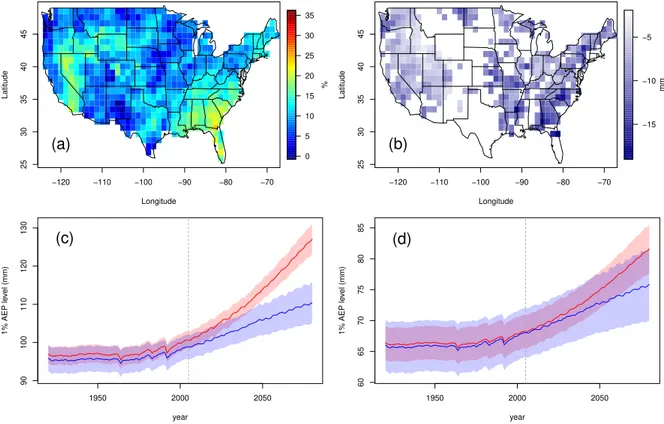
Although the GEV parameter estimates completely determine the fitted distribution of an-nual maximum daily precipitation, the parameters themselves have limited interpretability. Us-ing the parameter estimates, we are able to produce estimates of the 1% AEP level for any partic-ular year. Figure 2.2 shows 1% AEP level estimates for the years 2005 and 2080. These estimates range between 26.8-144.8 mm in 2005, compared to 32.6-164.6 mm in 2080. Standard errors calculated via the delta method (Coles, 2001, Section 2.6.4) range from 0.5-4.6 mm in 2080 (see Figure A.4). Between the years 2005 and 2080, the 1% AEP level is projected to increase for all grid cells under RCP8.5, with a U.S. median percentage increase of 17%. Changes in magni-tude are most noticeable in California and along the Eastern seaboard, but percentage changes (Figure 2.2(c)) are also more than 30% in the Basin and Range area of the west where current levels are quite low. Another way to understand the change in extreme precipitation is to con-sider the annual exceedance probability for a given level of daily precipitation, say the 1% AEP level in 2005. Under RCP8.5, the 2005 1% AEP level corresponds to a higher annual exceedance probability in 2080 across the contiguous U.S. (Figure 2.2(d)). In some areas such as southwest-ern Idaho and southsouthwest-ern Appalachia, a 1-in-100-chance event in 2005 is projected to become a 1-in-15 or higher chance event in 2080.
2.3.2 Comparison with CESM-ME (RCP4.5)
Parameter estimates and standard errors forµ4.50 (s),µ4.51 (s),φ4.50 (s),φ4.51 (s), andξ4.5(s) based on CESM-ME are obtained for all grid cells in the contiguous United States (see Figure A.5). Maps of estimates forµ4.50 (s),φ4.50 (s), andξ4.5(s) (Figure A.5(a), (e), and (i)) are very similar to those estimated from CESM-LE. On the other hand, estimates of the slope parametersµ4.51 (s) andφ4.51 (s) differ somewhat from those based on CESM-LE. Plots of these differences are given in Figure A.6(c) and (d). Null hypotheses ofµ4.51 (s) ≤ 0 and φ4.51 (s) ≤ 0 are still rejected in over 90% of the grid cells (Figure A.6(a) and (b)), agreeing with our finding from CESM-LE that the