Influence of spatial variation in precipitation on artificial neural network
rainfall-runoff model
André Dozier1
Department of Civil and Environmental Engineering, Colorado State University
Abstract. Modeling rainfall-runoff processes is a very challenging task due to data collection,
time, money, and technology constraints. Artificial neural networks (ANNs) are modeling tools that can quickly adapt and learn input-output relationships for many different engineering prob-lems. An Elman-type recurrent ANN was trained to simulate observed streamflow for Fountain Creek at Pueblo, CO, using varying amounts of spatial precipitation information. Nine zones were originally delineated within the watershed draining to Fountain Creek at Pueblo based on estimated overland flow travel time. Five different spatially varying scenarios were modeled: scenarios con-taining 9 zones, 6 zones, 3 zones, 2 zones, and 1 zone. Each scenario was trained and simulated 100 times, each with randomly generated initial weights. Spatial variability in precipitation data al-lows the ANN to achieve better performance when simulating the training dataset. However, when applied to the validation and testing time periods, ANN performance generally decreases with addi-tional spatially variability. In addition to exploring results of the ANN rainfall-runoff model, the application of geographical information systems to rainfall-runoff input processing is demonstrat-ed.
1. Introduction
Rainfall-runoff processes are highly complex. Spatial atmospheric conditions drive precipitation occurrence and type (snow or rain). Rainfall abstraction (the amount of pre-cipitation initially lost to evaporation), infiltration, overland flow, groundwater flow, flow accumulation, and flow transfer are all very complicated processes to model accurately due to lack of full spatial terrain datasets (soil, slopes, vegetation, etc.) and accurate forcing da-tasets (precipitation, temperature, solar radiation, etc.).
Data collection for preparation of a physically-based model is a problem both due both to the vast amount of spatial data to be collected and the inability to collect accurate data without altering the modeling environment. Nonintrusive and remote sensing techniques have aided in estimating spatially-varying soil, groundwater, and climatic data, but as with any estimate, errors and noise in the “measurements” are inevitable. So, because of data collection requirements and challenges and also because of the complexity of associated processes, many empirically-based techniques for rainfall-runoff modeling have been de-veloped. Each empirically-based technique is generally only useful for particular geo-graphical locations or characteristics and not generalizable.
1 Water Resources Planning and Management Division College of Engineering
Civil Engineering Department Colorado State University Campus Delivery 1372 Fort Collins, CO 80523-1372 Tel: (970) 491-7510
As an alternative approach, artificial neural networks (ANNs) have been used to repre-sent the rainfall-runoff process with a fair degree of accuracy. Tokar and Markus (2000) describe an improved performance of ANNs over conceptual models. ANNs seem to pro-duce streamflow output more representative of observations and to do so more consistently than conceptual models. The same ANN structure with different synapse signal strengths, or weights, may represent many different rainfall-runoff processes. An ANN was set up to represent rainfall-runoff processes with spatially varying precipitation inputs for Fountain Creek in central Colorado. Figure 1 displays the location of Fountain Creek along with ma-jor water-bodies, streams and elevations.
2. Data Acquisition
Figure 1. Fountain Creek location map.
Geospatial data utilized in applying a rainfall-runoff model to Fountain Creek included a 30-meter resolution digital elevation model (DEM), hydrography (stream flowlines and sub-basin outlines), a land cover dataset, spatial precipitation estimates, and streamflow at various locations. Hydrography and DEM data for hydrologic region 11d were obtained from NHDPlus data online at http://www.horizon-systems.com/nhdplus/ , provided by Horizon Systems Corporation. Land cover data came from the National Land Cover Data-base (NLCD) at http://gisdata.usgs.gov/ , a service of the U.S. Environmental Protection Agency (EPA). Spatial precipitation estimates were obtained from National Oceanic and Atmospheric Administration (NOAA). Streamflow gauging site locations were obtained also from the NHDPlus website mentioned above. Measured streamflow at each gage were then downloaded from the U.S. Geological Survey (USGS) website at
3. Procedure and Methods
Geospatial data was processed to provide inputs to the ANN modeling study. Overland flow time was estimated to serve as a delineation of zones, which would represent various degrees of response from the system. Average spatial precipitation was calculated within each zone. Precipitation constituted inputs to an ANN, which was built, trained, and then tested against measured streamflow estimates. This section outlines the procedures and methods that were used to develop and evaluate the ANN rainfall-runoff model.
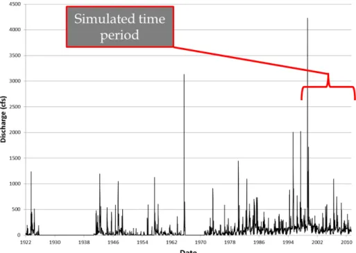
Spatial precipitation rasters were summed from hourly to weekly precipitation esti-mates. Daily streamflow data were also summed to weekly. April 1999 through August 2010 was the selected time period of analysis. A weekly timescale was selected arbitrarily, but we recognize that timestep selection may play an important role in conclusions of this study. Streamflow at the selected gauging location is displayed in Figure 2.
Figure 2. Historical streamflow in Fountain Creek at Pueblo.
Since ANNs are data-driven models, observed streamflow is required to train and test an ANN. A longer, accurate, and representative dataset is usually beneficial in order to train and test the ANN. Therefore, upstream streamflow gages with more than 5 years of recent data were selected by using the “Select by Attribute…” tool within ArcGIS after clipping to gauging locations only within the upstream region. Figure 3 displays the selec-tion of streamflow gauging locaselec-tions within the upper Arkansas River Basin. All gages displayed on the right within Figure 3 have more than 5 years of recent streamflow data within the basin.
Figure 3. Selection of potential streamflow gauging locations for rainfall-runoff analysis. After potential streamflow gages were located, watersheds were produced using the Batch Watershed Processing Tool within ArcHydro tools of ArcGIS. Pits were filled in the DEM to disallow ponding in flow direction calculations. Hydrography flowlines were then “burned” or embedded into the DEM in order to ensure that calculated flow direction and flow accumulation represent true stream locations. Then, flow direction and flow accumu-lation were calculated from the DEM. Geospatial locations of streams, catchments, drain-age lines, and adjoint catchments were derived. Finally, stream gauging locations were uti-lized as “Batch Points,” or watershed outlet points, for the Batch Watershed Processing Tool, which was accomplished by adding appropriate fields to the stream gage shapefile attribute table: “Name”, “Descript”, “BatchDone”, “SnapOn”, and “SrcType”. The batch watershed processing tool delineated 118 watersheds as shown in Figure 4.
Figure 4. Stream gauging locations (left) and final delineated watersheds (right) within the upper Arkansas River region.
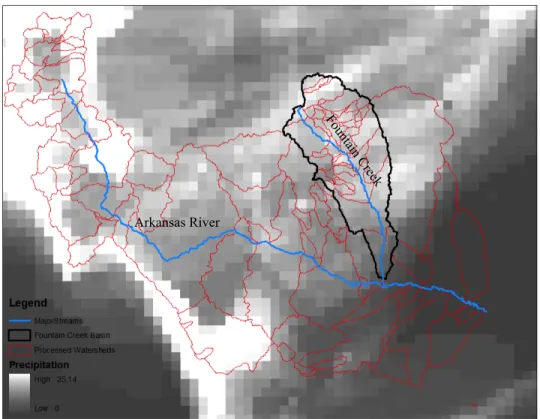
A mesoscale basin was selected based on the spatial variability of precipitation magni-tude within the basin. Fountain Creek Basin was selected as illustrated in Figure 5 because it is not snowmelt-dominated and is large enough to encapsulate a lot of spatial variation in rainfall. The basin has an area of about 2400 km2.
Zones within Fountain Creek Basin were delineated based on approximated overland flow travel time, which was estimated using an algorithm outlined by McCuen (2004). Overland flow velocity was first estimated by (1). Average travel time per meter within each grid cell was estimated by taking the reciprocal of the velocity in (2) as follows:
𝑉!" = 𝑘!"∗ 𝑆!"!.! (1) 𝑡!" = 1
𝑉!" (2)
where 𝑉!" is the velocity (m/s), 𝑘!" is the overland flow coefficient (m/s), 𝑆!" is the average slope (rise over run), and 𝑡!" is the average travel time (s/m) within grid cell (𝑖, 𝑗). Esti-mates of the overland flow coefficient for a specific land cover type from U.S. Geological Survey (2010) were used.
Figure 5. Selection of a watershed based on spatial variability of precipitation (units are in hundredths of millimeters).
Travel time within stream reaches is back-calculated from Manning’s equation, where 𝑛/𝑅!/! was approximated as 0.024. Slopes within the basin below 0.001 were set to 0.001 in order to avoid invalid calculations. Then, total travel time is calculated as cost-weighted distance to the basin outlet which was calculated using the Cost Weighted Dis-tance algorithm described by Environmental Systems Research Institute (2011). Several grid cells throughout the watershed had total travel times that were very different than sur-rounding cells. Therefore, a filtering process using the majority value of 20 sursur-rounding cells smoothed the delineation of zones within the watershed. The total travel time grid was then reclassified into nine different classes. Mean precipitation for each zone was then estimated using zonal statistics tools within ArcGIS. Zonal delineation and mean precipita-tion per zone are displayed in Figure 6.
Figure 6. Zonal precipitation calculation: zone delineation (left), precipitation raster overlay (middle), and zonal mean precipitation (right).
Calculations of zonal mean precipitation were done at each timestep over the entire time period, for a total of 596 timesteps. Therefore, in order to avoid tenuous manual culations, a custom .Net tool within ArcGIS was developed to automate zonal statistic cal-culations within the basin. Figure 7 displays a screenshot of the tool created within ArcGIS for automatic calculation of mean zonal precipitation for all precipitation rasters within the specified time period.2
Figure 7. Custom ArcGIS tool for zonal precipitation calculation.
After all inputs were collected and zonal statistics for precipitation were calculated, an artificial neural network was built within MATLAB, due to its fairly extensive toolset in
2 A quick note about precipitation raster file extension: the “*.aux” extension was used to simply find raster files within the input directory location, but was then removed within the code when generating the raster dataset with ArcObjects, because to ArcGIS, a “GRID” file name must be specified without an extension, as opposed to specifying a TIFF or JPG file.
building, training, and simulating ANNs. Artificial neural networks have an input layer, a hidden layer, and an output layer. A mathematical transformation takes place on the inputs in the input layer via weights and biases in order to produce a desired output, when histori-cal output data is available. In order to “train” an ANN to produce similar outputs given a set of selected inputs, the ANN is placed into an optimization routine that attempts to as-sign weights to “synapses” in the network that minimizes deviations of simulated runoff values from observed. Selected inputs for this study were just weekly spatial precipitation estimates, 𝑷(𝑡), described above. Outputs used for the supervised learning process were weekly streamflow quantities, 𝑆(𝑡), at USGS gage on Fountain Creek at Pueblo (USGS gage number 07106500). The time period of analysis was from April 1999 to August 2010. As Figure 2 displays, streamflow in this time period is perennial (not intermittent, as it was prior to major developments at Colorado Springs) and very different than historical stream-flow with one of its largest gauged stream-flows occurring at the beginning of the modeled time period.
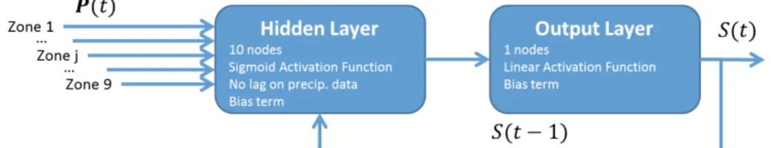
Due to the sequential nature of the problem, a dynamic, or recurrent, ANN was used, which provided feedback of streamflow from the previous timestep. A nonlinear auto-regressive with external input (NARX) neural network was used with 10 nodes in the hid-den layer and a sigmoid activation function, and 1 node in the output layer with a linear ac-tivation function. Also, since the model had a weekly timestep, only precipitation from the current timestep really affected streamflow, and therefore no lag was used with tion data. A model with a finer timestep, perhaps hourly, would require lagged precipita-tion estimates as inputs. A simple diagram of the ANN structure is displayed in Figure 8.
Figure 8. Diagram of recurrent ANN architecture. Figure taken directly from MATLAB interface.
A specialized backpropagation optimization technique known as Levenberg-Marquardt Backpropogation developed by Hagan and Menhaj (1994) was used to train the ANN. That is, the synapse weights were optimized to find the best simulation performance within the training period. Training the ANN was aimed at minimizing the mean squared error (MSE) of simulated streamflows when compared to observed streamflows. Additionally, though, overtraining can easily occur, where the neural network learns to imitate the training da-taset really well, but does not represent new dada-tasets well at all. Therefore, the ANN was trained on the first 70% of the observed streamflow within the modeled time period (April 1999 to August 2010), validated on the next 15%, and then tested on the last 15%. To avoid overtraining, the weights that performed the best in the validation dataset were used as the “optimal” weights as displayed in Figure 9. Thus, because the training algorithm does not seek a global optimum performance when compared with target streamflows in the training dataset, different “optimal” weights were found after randomly generating weights. The ANN was trained 100 times to capture a range of potential trainings and to
obtain an idea of the maximum performance within the training, validation, and testing pe-riods.
Figure 9. Selection of “optimal” network weights during ANN training.
In order to explore the importance of spatial variability in precipitation estimates as in-put to the ANN, five different scenarios were simulated: 9 zones of precipitation, 6 zones, 3 zones, 2 zones, and 1 zone of precipitation. In other words, at each timestep, nine differ-ent precipitation values were used represdiffer-enting precipitation at differdiffer-ent locations in the basin for the “9 zones” scenario. For the “1 zone” scenario, only one precipitation value was used for the entire basin. In order to quantify the improved capability of an ANNs to simulate streamflow with varying amounts of geospatial input information, each scenario was trained and simulated 100 times with randomly generated initial weights to get a range of potential trained neural networks over all three datasets (training, validation, and test-ing).
4. Results
Simulated streamflows from the ANN performed really well within the training da-taset, slightly worse in the validation dada-taset, and significantly worse in the testing dataset. Performance is evaluated with the Nash-Sutcliffe coefficient of efficiency (NSCE) and model bias (BIAS). NSCE accounts for the magnitude of error in addition to the variance. If the NSCE is equal to 0, the simulated output models the observed dataset just as effi-ciently as the average of the observed dataset. NSCEs can be negative meaning that simu-lated output performs worse than the average of the observed. An NSCE of 1 is the best possible value. BIAS indicates model over- or under-prediction by summing all errors. If BIAS is less than zero, the ANN model over-predicts observed streamflow; otherwise, it under-predicts.
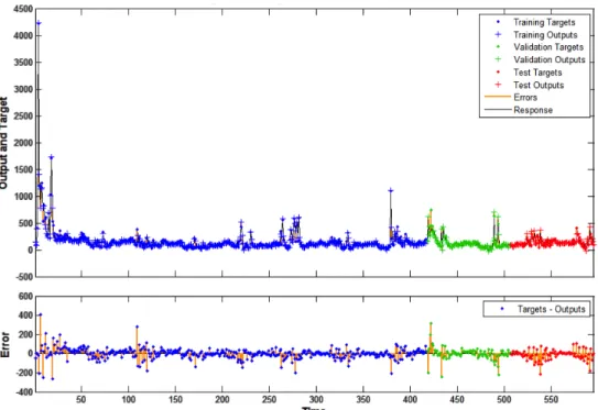
Figure 10. ANN streamflow prediction in cfs (top) and model residuals in cfs (bottom).
Figure 11. Simulated versus observed streamflow for all three datasets.
Model errors, or residuals, seem to indicate unbiased errors (although this is not statis-tically shown herein) and generally small magnitudes, even within the testing period. Fig-ure 10 displays streamflow predicted by the ANN after one training along with model
er-rors at each timestep. Also, Figure 10 illustrates the division of the training, validation, and testing datasets.
The ANN performs really well if evaluated over all three periods (training, validation, and testing). A NSCE of 0.95 was obtained for the trained ANN displayed in Figure 10. Figure 11 displays simulated output against observed output. Simulated output within the training dataset includes many of the higher peak flows. Altered datasets with higher peak flows within the validation or testing periods would be interesting scenarios to explore, but are not explored herein. Scaling the inputs and outputs for the training dataset would most likely have to be performed differently if the maximum or minimum flows occur outside of the training dataset.
Figure 12. Nash-Sutcliffe coefficient of efficiency (NSCE) values for 100 model train-ings within five spatially-varying scenarios, separated by training, validation, and testing datasets. Box-and-whisker displays outliers, maximum, 75th per-centile, median, 25th percentile, and minimum.
As mentioned above, five different scenarios were simulated: 9 zones of precipitation, 6 zones, 3 zones, 2 zones, and 1 zone of precipitation across the watershed. ANNs were trained and simulated 100 times for each scenario because initial weights were randomly generated. NSCE performance for each scenario and each dataset (training, validation, or testing) are displayed in Figure 12. BIAS was also calculated for each spatially varying scenario and is displayed in Figure 13. Intuitively, model performance decreases from the training dataset to the validation dataset to the testing dataset. It is important to note that any particular training may result in an excellent or even the best training performance, but
0 0.5 1 Training dataset 0 0.5 1 Validation Dataset Na s h -S u tc lif fe Co e ff ic ie n t o f E ff ic ie n c y , NS CE 9 6 3 2 1 0 0.5 1 Number of zones Testing Dataset
may perform poorly within the validation and testing datasets. So, no particular training will have the best performance in the training, validation, and testing periods.
Median and maximum NSCE values are fairly consistent between the 5 spatially vary-ing scenarios when observvary-ing the trainvary-ing period. However, in validation and testvary-ing da-tasets, less complex spatially varying information generally perform better. Model bias and error distribution seems to indicate that the model has no systematic errors within the train-ing and validation datasets. ANN simulation within the testtrain-ing period tends to over-predict because the training dataset contains wetter years and the testing dataset contains drier years.
Figure 13. Model bias (BIAS), or sum of errors, for 100 model trainings within five spa-tially-varying scenarios, separated by training, validation, and testing da-tasets. Box-and-whisker displays outliers, maximum, 75th percentile, median,
25th percentile, and minimum.
Maximum NSCEs for the validation and testing datasets are attributed to the scenario with 2 zones, which indicates that it is less likely to over-train an ANN with less spatial precipitation information (less input data, and consequently less weights over which to op-timize). However, this is only true given the assumptions and simplifications made within this model along with selection of the timestep. Table 1 lists median and maximum NSCE values for each spatially varying scenario (from 9 zones down to 1 zone) within training, validation, and testing periods. Figure 14 illustrates the difference between ANN simula-tions over the testing period with inputs divided into 9 zones and 1 zone. The less compli-cated structure, the scenario with 1 zone, performs better.
-2 0 2 Training dataset -2 0 2 Validation Dataset Su m o f e rr o rs * 1 0 -5 ( a c re -fe e t) 9 6 3 2 1 -2 0 2 Number of zones Testing Dataset
Table 1. Maximum and median NSCE values for different datasets with varying spatial precipitation information
Description Dataset 9 zones 6 zones 3 zones 2 zones 1 zone
Max NSCE Training 0.980 0.979 0.972 0.970 0.963
Validation 0.827 0.890 0.905 0.915 0.820
Testing 0.467 0.477 0.367 0.495 0.475
Median NSCE Training 0.955 0.938 0.939 0.946 0.935
Validation 0.640 0.671 0.823 0.821 0.756
Testing 0.056 0.070 0.078 0.254 0.295
Bold numbers indicate the best scenario for the particular criterion
Overall, the ANN that was trained using precipitation with only 2 zones seems to have the most desirable characteristics: not as likely to being over-trained, but exceptionally good performance within each of the datasets.
Figure 14. Observed and simulated streamflow for the testing dataset with either 9 zones of input precipitation (left) or 1 zone of input precipitation (right).
5. Conclusions
Rainfall-runoff processes are quickly and easily modeled with artificial neural net-works. Results seem to indicate that ANNs perform well during calibration, or training, but performance diminishes significantly when testing datasets that are completely disconnect-ed from the training dataset. When testing the capability of the ANN with various spatial precipitation inputs, the ANN performed consistently the same throughout each of the sce-narios within the training dataset. However, when testing on a new dataset, the ANN per-formed better with less spatial precipitation information. That is, the ANN tested better when given only one or two precipitation values at each timestep rather than nine. A finer timestep than weekly may significantly change this conclusion. Noise and cross-correlation between precipitation estimates could account for additional noise in the outputs of ANNs trained with multiple zones.
In addition to the conclusions about the application of an ANN to rainfall-runoff pro-cesses, this paper has demonstrated the use of Geographic Information Systems (GIS) to efficiently generate estimations of required input data for hydrologic models. Useful calcu-lations included DEM manipulation, batch watershed processing, cost-weighted distance,
500 510 520 530 540 550 560 570 580 590 600 -200 -100 0 100 200 300 400 500 600
Testing Period 9 zones, NSCE = -0.097542
Timestep Di s c h a rg e ( c fs ) Observed Simulated 500 510 520 530 540 550 560 570 580 590 600 -200 -100 0 100 200 300 400 500 600
Testing Period 1 zone, NSCE = 0.34886
Timestep Di s c h a rg e ( c fs ) Observed Simulated
table joins, and zonal statistics. A lot of zonal statistics calculations can be computationally expensive.
Many applications for ANNs within hydrology exist. However, the ANN described herein does not have direct applications beyond filling streamflow estimates on a previous-ly gauged site for which precipitation estimates exist. The ANN could be enhanced to es-timate streamflow at ungauged sites by training on many gauged sites while incorporating other geospatial or topographical information such as land cover, soil composition or cate-gorizations, land area, elevations, average slopes, curvature, vegetation, etc. Combined spatial and temporal interpolation capabilities of ANNs could then be explored.
Improvements to the design of the ANN could enhance its performance. Radial basis functions have a generalizing capability that makes them attractive for natural processes. Additionally, more temporal inputs could improve the performance of the ANN. For ex-ample, streamflows of other nearby gauging stations could also improve the performance of the ANN. Temperature would improve the ANN performance especially within snow-melt-dominated watersheds because temperature significantly impacts streamflow. Also, some type of conceptual input parameter such as a storage term might improve perfor-mance within large basins, basins with a lot of unregulated storage, highly irrigated river reaches, and snowmelt-dominated basins. Such storage parameters are used in conceptual models, but could be applied within an ANN as well.
Foreseen directions for future work on ANN rainfall-runoff modeling could include questions such as:
1. How well does the ANN perform with different training, validation, and testing da-tasets (perhaps leaving some of the high peak flows out of the training dataset)?
2. How well can the ANN perform with no current timestep information as input (only precipitation from previous timesteps being utilized – a finer timestep would need to be used)?
3. How does spatial variability affect an ANN’s streamflow predicting capability at smaller timesteps such as daily, hourly, or sub-hourly?
4. How well do ANNs predict streamflow with varying types of precipitation input (pre-cipitation estimates from rainfall gages)?
5. How well can the 100 differently trained ANNs perform ensemble prediction?
6. How does variation in types of spatial information affect an ANN’s streamflow pre-dicting capability (e.g., including other information such as temperature, elevation, land cover, number of pumping wells, length of canals and streams, etc.)?
7. How well can an ANN disaggregate seasonal or monthly precipitation estimates into daily or weekly streamflow (given other inputs)?
8. How well do ANNs fill in missing streamflow as compared to other techniques? 9. How well could the same ANN predict streamflow at another watershed given some
scaling factors? (train one ANN on lots of different streams throughout the world with inputs like area, temperature, elevation, upstream streamflow, stream length, snow ac-cumulation over winter period, etc.)
10. How can this process be automated to estimate streamflow at locations all over the U.S.?
11. How can this process be utilized within climate change hydrology studies to evaluate impacts to streamflow?
Acknowledgements. This research was performed in requirements for two classes within the Civil
& Environmental Engineering Department within the College of Engineering at Colorado State University. Therefore, the author acknowledges the instruction of Dr. John Labadie and Dr. Darrell Fontane, who provided the necessary background framework to accomplish the work described in this paper. Also, the author gratefully acknowledges Dr. John Labadie for the use of a computing laboratory.
References
Environmental Systems Research Institute, 2011: Understanding cost distance analysis. ArcGIS Resource
Center, http://help.arcgis.com/ en/arcgisdesktop/10.0/help/index.html#/Understanding_cost_distance _analysis/009z000000z5000000/ .
McCuen, R. H., 2004: Hydrologic Analysis and Design. Prentice Hall, Upper Saddle River, N. J., 3rd edition, 888.
Tokar, A. S., and M. Markus, 2000: Precipitation-runoff modeling using artificial neural networks and con-ceptual models. J. Hydrol. Eng., 5, 156-161.
U.S. Geological Survey, 2010: NLCD 92 Land Cover Class Definitions. The USGS Land Cover Institute