1
Determinants of women’s labour supply in Bangladesh and Pakistan
Ali Abbas
Department of Economics Master Thesis, Spring 2013 15 ECTS
2 Table of Contents Table of Contents ... 2 Acknowledgement ... 4 Abstract ... 5 1. Introduction ... 6
Objective of the study ... 8
Hypotheses ... 8
2. Literature Review... 9
3. Theoretical framework ... 13
Demographic transition model ... 13
Neoclassical model ... 15
4. Methodology ... 20
Estimated model... 20
Data ... 22
Vector Error Correction Model ... 22
The unit root test ... 24
Cointegration tests ... 25
5. Results ... 26
Unit root test ... 26
Johansen Cointegration ... 29 Bangladesh ... 29 Pakistan ... 29 VEC Estimation ... 30 Bangladesh ... 33 Pakistan ... 35
3
Impulse response ... 37
Bangladesh ... 37
Pakistan ... 39
6. Conclusion ... 42
Results for Pakistan... 46
4
Acknowledgement
I would like to thank my supervisor Gauthier, for his guidance, insights and invaluable comments throughout the writing of this thesis. A special thanks to all those who supported me in the writing of this paper.
5
Abstract
This thesis is about the determination of women’s labour supply in Bangladesh and Pakistan from 1980 to 2011. The study focuses on the demographic variables (infant mortality rate and total fertility rate), primary education rate, GGDP per capita growth and GGDP per capita growth square. The VEC model is used to estimate the relationship between variables, in the long run. Data are obtained from the World Bank. The results for both countries confirm the U-shaped pattern hypothesis between women’s labour supply and economic development. The results indicate that, in Bangladesh, a shock to infant mortality rate on women’s labour supply is more effective than in Pakistan, and that a positive shock to primary education on women’s labour supply is more effective in Bangladesh than in Pakistan. The results also show that a positive shock to total fertility rate on women’s labour supply in both countries has a similar impact.
Keywords: women’s labour supply; demographic variables; primary education; economic
6
1. Introduction
This thesis focuses on women’s labour supply in Pakistan and Bangladesh with special reference to demographic transition, fertility and infant mortality, women’s education and economic development. Data from 1980 to 2011 are used in this study due to the demographic transition over this period for both countries (see Appendix A). Mincer (1974; 1962) provided the foundation studies on women’s labour supply from the economic perspective. According to Guillermo and Quentin(2003) a family with a large number of children demands more time for child care activities, and, hence, reduces women's labour supply availability. Similarly, if the mortality rate is relatively high, there is a possibility of high childbearing. There is also a possibility for women to participate in the labour market even though the infant mortality rate is high, especially if the woman is the breadwinner of her family (Jamaly & Wickramanayake, 1996). One study notes that birth might reduce a woman's labour supply from the job market and takes almost two years of her reproductive life (Bloom, Canning, Fink, & Finlay, 2009).
According to Royalty (1998),women’s labour supply is closely related to their accessibility to education. The human capital theory states that women with a higher level of education participate more in the labour market than those with low or no education(Tomaskovic-Devey, Thomas, & Johnson, 2005). Education enhances the rate of women’s labour supply by increasing their eligibility criteria to fulfil job requirements (Tansel, 2002). A study by Achkah, Ahiadeke and Fenny (2009) notes that women with primary education are economically more active than those with no education. Their study finds that there is a strong positive relationship between education and women’s labour supply, particularly for those who had completed their primary education. Women’s
7
education has a significant effect on low fertility and late marriage, and greatly improves child health and nutrition (Todaro, 1994).
Women’s labour supply is essential for their family's survival as it increases household income(Anker, 1983; Kelly, 1986; Mincer, 1962). The literature shows that the relationship between women’s labour supply and economic development is U-shaped (Goldin, 1994; Tansel, 2002; Tanveer & Elhorst, 2008). In the initial stage of developing economies, when income is extremely low, women largely work in the agriculture sector, for example, farming, poultry farms and cultivation. They are either paid less or work as unpaid workers on their family farms along with child caring and other domestic responsibilities. As income increases, mainly due to the expansion of the market or the introduction of technology, a structural shift from agriculture to industry causes a decline in women’s labour supply. This may be because of the low education level of women as well as the shift in the work place from family-based environment to the market (Al-Qudsi, 1998) . Moreover, women’s labour supply increases in high income economies since women have better education and there are more job opportunities for women.
This thesis is particularly interested in the demographic transition in Bangladesh and Pakistan, and the evolution of women’s labour supply. Historically, Bangladesh and Pakistan were one country and shared the same culture and norms. Later, in 1971, they were divided into two countries. Moreover, both countries are ranked among the top ten labour producing countries (Mazhar, 2013). In addition, studies on the research focus, comparing the data from these two countries, are limited and the topic remains underexplored. It is important to note that women’s participation in the market helps to improve their status and brings them into
8
the household decision making concerning the number of children they bear and enhances household income (Muhammad & Fernando, 2010).
Objective of the study
The main objective of the study is to investigate the determinants of women’s labour supply in Bangladesh and Pakistan from 1980 to 2011, in respect of demographic transition. Primary education and economic development are also employed as variables.
Hypotheses
1) A lower infant mortality rate (IMR) increases women’s labour supply (WLS). 2) A lower total fertility rate (TFR) increases women’s labour supply (WLS).
3) The relationship between economic development and women’s labour supply (WLS) has a U-shape.
4) A higher primary education completion rate (EDU) increases women’s labour supply (WLS).
This thesis is structured as follows. Section II discusses the review of the literature and briefly explains the variables used in the study. Section III presents the theoretical framework and model. Section IV explains the methodology and in section V the results are presented. The last section provides the conclusion of the study.
9
2. Literature Review
The study on Nigeria by Ashraf, Weil and Wilde (2013) concerns the effect of fertility and its relationship with the gross domestic growth per capita. The study uses the United Nations (UN) medium-fertility population projection as a baseline. The study confirms that a decline in fertility increases the income per capita by an amount that can be considered as economically significant. Moreover, the study indicates that shifting from the United Nations (UN) medium-fertility population projection to the low-fertility population projection raises income per capita by 5.6 per cent within 20 years, and 11.9 per cent within 50 years, which is economically accepted.
A comparative study by Doepke (2004) in England, South Korea and Brazil shows that the decline of fertility in all developed and industrial countries was accompanied by a demographic transition from high to low fertility. The overall repetition process in cross-country varies and also depends upon the speed of the demographic transition. The main finding shows that education and child labour policies affect fertility during the transition to growth. For example, if parents have to pay school fees and child labour is unrestricted, fertility transition starts later and progresses slowly. On the other hand, fertility reduces rapidly if the education is publicly provided and child labour is illegal (Nanjunda, 2009).
The study conducted on women’s labour force participation and fertility of high, medium and low income countries by Nguyen (2009) concludes that fertility has a negative relationship with women’s labour supply. The study uses two-stage least squares to analyse the data, and shows that the decline of fertility enhances the women’s participation in the labour market in all countries. The study also notes other factors, such as attainment in
10
education and economic development that encourage women’s labour supply. For example, if a woman acquires education, her participation in the labour market is more valuable than those without or less education.
On the other hand, several studies note that economic development has a positive relationship with fertility, for example, Thyrian et al.(2010) and Andersson (2000). Their studies demonstrate that it is also possible for highly educated mothers with high income to have high fertility due to the encouragement policies by the authorities, such as maternity and paternity leave policy and paid salaries after giving birth to a child. A study in Greece by Hondroyiannis and Papapetrou (2002) examined the industrialized situation and the reasons for the decline of fertility rates by analysing the period from1960 to 1990. The study indicates that an increase in real GDP per capita due to productivity improvements will lead to higher fertility. Through analyses of the vector error correction model (VECM), the variance decomposition analysis and impulse response function confirms the endogeneity of the fertility rate in a joint dynamic relationship.
Fertility rate, education, and women’s labour supply
According to Singh (1994), the neoclassical theory explains that the increasing investment in human capital may encourage women's work transition from unpaid work, such as domestic chores, to wage-paid jobs. These changes affect household fertility choices and urge parents to moderate the number of children. The decline of fertility is associated with an increase in human investment in the shape of education. For example, the study conducted by Salehi-Isfahani and Kamel (2006) shows that Iran experienced a sharp fertility decline in the 1990s. The Iranian fertility rate declined from more than six births to about two births per women between1980 and2004. Significantly, Iran’s childhood education programme was greatly
11
expanded, and attained the first position in the Middle East in preschool enrolment. Moreover, for the same period, the kindergarten enrolment increased from less than 0.1 per cent to nearly 1.5 per cent of all children who were five years old. The results affirm that family choice has changed and that it affects the shape of the decline of fertility and increase in investment. Consequently, the school going children reflect the parents substitute behaviour between quality and quantity. A substantial growth in total factor productivity and reduced poverty is closely linked to the improvement in schooling, child mortality and adult health, particularly in low income countries (Schultz, 1994). Harmon, Oosterbeek & Walker (2003) conducted a study on human capital in terms of the benefit of education using the regression method and the log wage equation along with controls for work experience and other individual characteristics. They concluded that an individual income has a positive relationship with his/her participation in education. By investing in education, it assists a person to improve skills, which turn into human capital and increases his/her value in the society. Women's education is as important as male education and may have a higher rate of return, in that an increase in labour force participation along with an increase in farm productivity, low fertility and late marriage, greatly improves child health and nutrition (Todaro, 1994). Educated mothers can look after their children better and can improve the quality of human capital for future generations (Todaro, 1994). In addition, educated mothers are likely to emphasise an increase in the children’s schooling, which will result in a reduction in the infant mortality rate and fertility rate; all such factors are important for a healthier society (Subbarao & Raney, 1992). Women’s education significantly enhances the importance of women’s participation time in the society/market as well as for domestic chores. A study in Pakistan, by Muhammad and Fernando (2010), based on the structural model equation and path model examined the status of women in relation to the fertility rate. The study argues that the low status of women is the major root of the high fertility in
12
Pakistan. A comparison of the status of rural-urban women shows that a rural woman has less rights in household decisions compared to urban women. Urban women have more opportunities to gain an education and have better earning prospects. Consequently, urban women improve their status and take a role in household decisions. The study also finds a negative relationship between the status of women and fertility in Pakistan. The study of Ganguli et al. (2011) shows that by giving women the same level of education as men, it increases women’s participation in the economy and helps to narrow down the gender gap. Based on the study by Fatima and Sultana (2009) it is believed that by increasing the education level among women and improving the Pakistan economy, women will be encouraged to join the labour force.
13
3. Theoretical framework Demographic transition model
The demographic transition and neoclassical growth theories are used in this thesis to understand the research topic. The demographic transition theory helps us to understand the dramatic changes of fertility and mortality and their effects on women’s labour supply in respect of economic development. In addition, the macroeconomic human capital growth model is used to see its effect on the demographic variables (infant mortality rate and total fertility rate) related to women’s labour supply (Tamura, 2006).
The demographic transition model predicts how the demographics change as the economy develops. The theory mainly focuses on the changes in the rate of mortality, birth rate and the effects on economic development. There are five stages of demographic transition.
The first stage explains the phenomenon of high birth rate as well as the mortality rate. This period commonly happens when a country is still dependent on agriculture as its main economic activity. During this period, the family commonly has many children, mostly due to their need for labour to help with farming their fields and for their support during their old age. The family might also lack knowledge concerning family planning and contraception. Similarly, the infant mortality rate is also high during this time because of the low household income. Because of the low household income a family is unable to afford
14
better health care facilities for the members of their family, such as prenatal care and ultrasound. The family might choose to have traditional midwifes rather than professional health care providers. Moreover, the lack of the technological advancement in health care, for example, to prevent premature births and improve care of premature babies, might contribute to the high infant mortality rate (Richardson et al., 1998). The high rate of infant mortality could also be a possible reason for the high birth rate, as a family who has a child mortality might ‘replace’ the child by having another (Al-Qudsi, 1998; Hondroyiannis & Papapetrou, 2002).
In the second stage, the demographics change, as although the fertility rate remains at the high level, the mortality rate rapidly decreases due to the improvement in health facilities and education. Consequently, the population size increases. In the third stage, the mortality rate continues to decrease at a lower rate than that prevailing during stage two. In this stage, the improvement of health facilities allows the family to have the number of children they need without having infant mortality. Also, in this stage, economic structural change mitigates a family’s need to have fewer children. Therefore, the fertility rate is now at its lowest.
In the fourth stage, fertility falls below the level of the mortality rate. Hence, the number of the population either slowly increases or is stable. The reasons behind these changes could be due to access to contraception or the high cost of living to raise children. Researchers have stated that at this stage, women have more access to education, and that it allows women to choose a career. Consequently, it affects their decision to marry and have children at a later age, and, hence, the size of the population starts to level off.
15
In stage five of the model, the size of the population starts to decrease slowly as the birth rate is lower than the mortality rate even though health facilities are getting better. Most researchers emphasize that the reason behind the changes could be due to family planning, the high cost of living, marriage at a later age and women’s decision to participate in the labour market as well as their decision to choose a career rather than motherhood (Kirk, 1996).
Neoclassical model
The neoclassical growth model is considered as one of the fundamental pillars of the economic development theories. This theory helps us to understand how static economic growth can be obtained through three important factors –capital, labour and technology – in a discrete and continuous time framework. Solow and Swan published their articles in the same year (Solow, 1956; Swan, 1956) and introduced the Solow-Swan Model, or simply the Solow Model. Prior to the Solow model, Harrod-Domar introduced the economic growth model in their article, which later became the most common approach to study economic growth. By using the Leontief production technology, Harrod-Domar developed the most popular and simplest theory, which emphasizes the supply side effect, due to an increase in productive capacity through investment. The model takes the exogenous growth of the labour force (n), constant capital to labour ratio and capital to output ratio. The model further continues with the constant assumptions and considered returns to scale and returns to capital as constants. The model concludes that the higher the saving rate and the lower the capital to output ratio, the faster an economy grows.
Many economists have voiced disagreement and criticised the Leontief production function assumption of using fixed factors of production, and ignoring the imperfect
16
substitutability between the factors. The imperfect substitutability was criticised on the basis that in labour surplus countries it could be replaced with capital and vice versa. Moreover, it has also been argued that a low growth rate may be the reason for the lack of capital productivity rather than a constraint over the availability of capital (low investment). They further said, that to attain the equilibrium, the assumption of fixed capital to output ratio should relax, and, hence these should grow at the same rate(Snowdon & Vane, 2005).
This dissatisfaction provides the reason to replace the Leontief production function with the neoclassical growth theory. In the neoclassical growth theory, total production is a function of labour, capital and technology over a period of time. The Solow model considers the rate of saving, population growth rate and technology progress as exogenous. The model assumes the idea of perfect substitutability among the factors.
Furthermore, human capital is also included in the Solow model to analyse its impact on the economic growth theory (Acemoglu, 2007). Human capital can be defined as the stock of skill, education and other productivity-enhancing characteristics embedded in labour. In fact, the concept and the term human capital can be understood by an individual’s investment to develop and improve their skills and competencies. The idea of investment in human capital is derived from a firm, such as investment in the physical capital to increase their productivity. Mincer & Polachek (1974), and Becker (1965) came up with the pioneer idea of family investment in human capital and women’s labour supply. For now, it is important to understand the difference between hours supplied by individuals according to their efficient unit which is not the same. For example, a woman, as a skilled factory worker, can produce a product within a few hours while an amateur would spend much more time to perform the same job. Thus, on the basis of this example we conclude that a skilled factory worker with
17
efficient units of labour embedded in the labour hours she supplies, or, alternatively, more human capital, can help her to perform the task faster than an amateur.
The theory of human capital is vast, however, our objective is more modest, that is, to investigate the impact of human capital on women’s labour supply in the context of demographic transition variables, such as fertility and infant mortality with a succinct link with economic development. Tamura's (2006) study shows the succinct link between the effect of human capital on infant mortality and fertility. According to him human capital helps a mother to reduce infant mortality (e.g. mothers induce their children to wash their hands before meals, which probably helps them to avoid diseases) which, in turn, results in lower fertility. Therefore, lower fertility reduces the cost of human capital, and, consequently, allows parents to increase human capital investment on each child and provide time for women to work in the labour market.
Human capital constitutes one of the three main variables for income difference – physical capital, human capital and technology. For the purpose of this section, we consider that in a continuous time period, the economy total production function in the Solow growth model looks like:
[ ]Equation 1
Where Y is the total amount of production of the final good, in continuous time period
t, K is defined as capital stock, L is labour, A is measure of knowledge.(AL is labour –
augmenting technological progress) and H denotes "human capital". How it is measured in the data will be discussed below. As usual, we assume throughout that A> 0.
Assumption 1Says: The production function F is twice continuously differentiable in
18 ( ) ( ) ( ) ( ) ( ) ( )
Moreover, F exhibits a constant return to scale (CRS) in its three arguments
Assumption 2: F satisfies the Inada conditions. (The Inada conditions states that: the
"first unit" of capital, human capital and labour is highly productive, but after reaching a sufficient level their marginal products are close to zero).
( ) and ( ) 0 for all H>0 and AL>0, ( ) and ( ) 0 for all K>0 and AL>0, ( ) and ( ) 0 for all H>0 and AL>0.
Moreover, it is assumed that household investment in human capital is similar to the investment in physical capital. Hence, households save a faction of their income to invest in human capital and they save a faction to invest in physical capital. Both physical and human capital depreciate at a constant rate. The depreciation rates are denoted by and , respectively.
It is further assumed that there is a constant population growth rate and a constant rate of labour-augmenting technological progress, i.e.
̇
19
Where n and g are exogenous parameters and where a dot over the variables defines a derivative with respect to time. The growth rate of a variable reflects in its proportional rate of change.
Now defining effective human and physical capital ratios as:
The model assumes a constant return to scale feature in Assumption 1, and the output per effective unit of labour can be written as:
̂
( )
[( ]
Law of motion
Generally, output is divided between consumption and saving in a closed economy. The fraction of output allocated to investment, , is exogenous and constant. It is supposed that one unit of output allocated to investment yields one new unit of capital (either).In addition, the existing capital depreciates at the rate of φ. The law of motion for human capital (h) and physical capital can be written as:
̇( ) ( ) ( ) ̇ ( ) ( )
Finally we can conclude that a unique steady state exists when the Solow growth model is augmented with the human capital. Referring to the cross country behaviour, it is considered that a country with greater propensity to invest in human capital will have better economic growth compared to the others, even though they are experiencing the same progress in labour augmented technologies, g.
20
4. Methodology
Estimated model
The theory allows us to specify an economic growth model in continuous time period.
( )Equation 2
Lm and Hm represent the male labour force and (male) human capital, respectively, while Lw
and Hw represent women’s labour supply and (women) human capital, respectively. N (t)
represents population growth rate. As the study’s focus is (women) labour supply, we do not include capital in the model and assume capital is growing at a constant rate.
Equation 3
As the main focus of the study is about women’s labour supply we assume that male labour force and (male) human capital is given in the economy and increasing at a constant rate. lnY2 is also included in (equation 3) to capture possible non-linearity in income. Let y is a vector of GDP per capita and GDP per capita square, women labour supply, women's education, total fertility rate and infant mortality rate. Final equation 4 looks like:
Equation 4
and represent the output of a country (gross domestic product per capita, and gross
domestic product per capita square of country j at time t) and are used as a proxy for a country’s economic development. Other variables include Lw, which is the measure of
21
women’s labour supply, Hw, which is measured in terms of women’s primary education, and
N, which is measured by the proxy for total fertility rate and infant mortality rate. The value
of represents the intercept of the model. We use the natural log for all the variables as it is easier to work with.
22
Data
Time series data compiled from 1980 to 2011 from the World Bank website are used to estimate the empirical model for both countries –Bangladesh and Pakistan. The data for thirty-two years are used in this study; firstly, due to the accessibility of the data, and, secondly, in this time period, demographic transition occurred in both countries. Both Bangladesh and Pakistan are developing countries and rank in the top 10 labour supply countries. In Pakistan, the ratio of women in the total population is more (51%) than for men (Mazhar, 2013), while in Bangladesh the ratio between genders is almost the same (50%) (Bangladesh Bureau of Statistics, 2011). We use primary education as a proxy for human capital and GDP per capita as a proxy for economic development. Definitions of the variables are provided in appendix A. The student package (Software) Eviews 7 is used to estimate all the calculations.
Vector Error Correction Model
This study uses the vector error correction model (VECM). The VEC model is a restricted form of the standard autoregression (VAR) model. Studies confirm that Vector
Auto-regression (VAR) is considered as one of the most reliable frameworks when estimating joint dynamic and interdependence of macroeconomic and demographic multivariable time series (Engle & Yoo, 1989; Hondroyiannis & Papapetrou, 2002; Lewis, 2010). As the VAR model is not restricted with any theoretical input, it is considered as being a good choice in estimate studies where there is uncertainty regarding the choice of endogenous and exogenous
variables. The VAR technique considers variables as endogenous and allows their past and present information to affect each other (Greene, 2009). A VAR model can be used to analyse after a series is reduced to stationarity by investigating at differencing and other
23
transformations, such as seasonal adjustment (Greene, 2009). According to Lewis (2010), both VARs and VECs are useful tools to conduct analyses for the long-term, as well as short run dynamic relationships among non-stationarity variables. As suggested in VAR (Greene, 2009), the model treats all the variables as endogenous variables in the dynamic system (and hence tests for that endogeneity). A VEC model is used when all the variables of VAR are associated in the long run and cointegrated at the same level. The error corrections and cointegrating relations are particular to VECs. The VEC model used to estimate the equation can be represented by the following system of equations
Equation 5
Where q,d and t refer to the number of cointegrating relations (the cointegrating rank), specified lag length in variables difference, and time (year). Where y is the vector of endogenous variables (i.e. GDP, GDP2, IMR, TFR, EDU), υ stands for residuals from the estimated cointegrating equations (such as deviation from the long run); shows the (short-run) speed of convergence or adjusted parameters to be estimated; β on the right side of the equation stands for the coefficients to be estimated, and ε are the disturbance terms, assumed to be white noise (however, it may be correlated across equations).
The procedure used here for estimating the VEC follows four distinct steps. The first step is to ascertain the non-stationarity properties of the variable. The next step is to determine the cointegration among variables, and, third step estimate the cointegration (error correction) model and finally, (forth step) innovation accounting (i.e. impulse response analysis).
24
The unit root test
To determine the causal relationship between the women’s labour force participation and the explanatory variables (as mentioned earlier) selected for the study, the econometric technique demands choosing the best suitable econometric model for the study. The unit root test is consistently used in the linear regression model to detect the presence of stationarity and non-stationarity in the data (Phillips, 1987), since it tells about the non-stationarity/non-non-stationarity in the data; for example, whether the variable is stationary/non-stationary either at level or first difference. In the present study the unit root is investigated using the Augmented Dickey Fuller (ADF) test, which consists of three sets of equations.
- ∑ - Equation 6
Where from Equation 6, βo is the intercept, Yt is the current value of time series
variables, and is linearly dependent on the constant term βo plus Yt-1, the previous year value, t is the trend and error term µt. To detect whether the equation does contain non-stationarity
or not, we run the regression and test the hypothesis, that is, Ho: Ω=0, alternative H1: Ω<0
determines the unit root. (Asteriou & Hall, 2007).
By using the Augmented Dickey Fuller (ADF) test, each variable is tested through level and first difference to confirm the stationarity in the data; hence, spurious regression can be eliminated by this process. The results presented in the table show that the level coefficient of each variable in both countries (Bangladesh and Pakistan) are non-stationary. Hence, all the variables of each country are tested at first difference; the results confirm that all the variables of both countries are stationary at first difference I (1) with a lag value equal to zero.
25
Cointegration tests
The spurious regression from unit root, which explains that if two variables are non-stationary then we can represent the error as a combination of two cumulated error process, and that these error processes are often called stochastic trends. In other words, we can predict that their combination could produce another non-stationary process.
However, in a special case, if X and Y are really related, then we would expect that they will move together and so the two stochastic trends would follow a similar trend to each other, and, at the time of their combination, it should help to eliminate the non-stationary. In the special case we consider that the variables are cointegrated. The theory defines this condition as only when there really is a relationship between two variables, and so cointegration becomes a very powerful way to detect the presence of economic structure.
The cointegration is used to detect if there is a long run association ship among the variables and they cannot move independently. The Johansen cointegration test is applied to find the existence of a long run association among the variables in the model (Asteriou & Hall, 2007).
Hypothesis
H0: r = 0 (There is no cointegration) H1: r≤1 otherwise.
26
5. Results
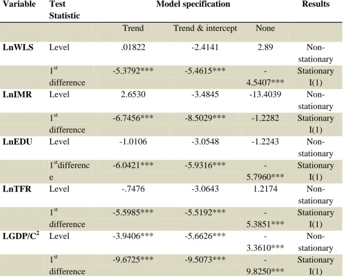
Unit root test
Table 1 Bangladesh (Unit root test)
Variable Test Statistic
Model specification Results
Trend Trend & intercept None
LnWLS Level .01822 -2.4141 2.89 Non-stationary 1st difference -5.3792*** -5.4615*** -4.5407*** Stationary I(1)
LnIMR Level 2.6530 -3.4845 -13.4039
Non-stationary
1st
difference
-6.7456*** -8.5029*** -1.2282 Stationary I(1)
LnEDU Level -1.0106 -3.0548 -1.2243
Non-stationary 1stdifferenc e -6.0421*** -5.9316*** -5.7960*** Stationary I(1) LnTFR Level -.7476 -3.0643 1.2174 Non-stationary 1st difference -5.5985*** -5.5192*** -5.3851*** Stationary I(1) LGDP/C2 Level -3.9406*** -5.6626*** -3.3610*** Non-stationary 1st difference -9.6725*** -9.5073*** -9.8250*** Stationary I(1) level :1per cent, 5per cent & 10per cent, respectively,***,**,*. Values are Intercept: -3.6661, -3.6661, -3.6661,-3.6661.Trend & Intercept: -4.2949, -4.2949,-4.2949,-4.2949.None: -2.6423,-2.6423,-2.6423, -2.6423
27 Table 2 Pakistan (Unit root test)
Variable Test
Statistic
Model specification Results
Trend Trend & intercept None
LnWLS Level 0.01822 -2.4141 2.8985*** Non-stationary 1st difference -5.3792*** -5.4615*** -4.5407*** Stationary I(1)
LnIMR Level 2.6530* -3.4845* -13.4039
Non-stationary
1st
difference
-6.7456*** -8.5029*** -1.2282 Stationary I(1)
LnEDU Level -1.0106 -3.0548 1.2243
Non-stationary 1stdifferenc e -6.0421*** -5.9316*** -5.7960*** Stationary I(1) LnTFR Level -0.7476 -3.0643 1.2174 Non-stationary 1st difference -5.5985*** -5.5192*** -5.3851*** Stationary I(1) LGDP/C2 Level -0.9946 -2.9548 -1.4283 Non-stationary 1stdifferenc e -5.4328*** -5.3354*** 5.2161*** Stationary I(1) level:1per cent,5per cent& 10per cent, respectively,***,**,*. Values are Intercept: -3.6661, -3.6661, -3.6661,-3.6661.Trend & Intercept: -4.2949, -4.2949,-4.2949,-4.2949.None: -2.6423,-2.6423,-2.6423, -2.6423
By using the Augmented Dickey Fuller (ADF) test, each variable is tested through level and first difference to confirm the stationarity in the data. Hence, spurious regression can be eliminated by this process. The results presented in table 2 and 3 show that at level, all coefficients of each variable in both countries (Bangladesh and Pakistan) are almost non-stationary, which means the null hypothesis can be accepted (refer to Table 2 and Table 3). Finally, all the variables for each country are separately tested at first difference; the results
28
confirm that all the variables for both countries are stationary at first difference I (1) with a lag value equal to zero.
29
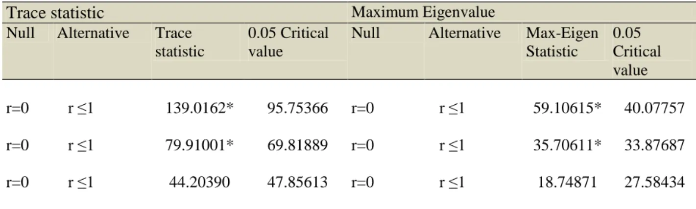
Johansen Cointegration
Bangladesh
Table 3. Johansen Cointegration Test Results
Trace statistic Maximum Eigenvalue
Null Alternative Trace statistic
0.05 Critical value
Null Alternative Max-Eigen Statistic 0.05 Critical value r=0 r ≤1 139.0162* 95.75366 r=0 r ≤1 59.10615* 40.07757 r=0 r ≤1 79.91001* 69.81889 r=0 r ≤1 35.70611* 33.87687 r=0 r ≤1 44.20390 47.85613 r=0 r ≤1 18.74871 27.58434
* denotes rejection of the hypothesis at the 0.05 level
Pakistan
Table 4. Johansen Cointegration Test Results
Trace statistic Maximum Eigenvalue
Null Alternative Trace statistic
0.05 Critical value
Null Alternative Max-Eigen Statistic 0.05 Critical value r=0 r≤1 152.3266* 95.75366 r=0 r≤1 53.71867* 40.07757 r=0 r≤1 98.60791* 69.81889 r=0 r≤1 37.67552* 33.87687 r=0 r≤1 60.93239* 47.85613 r=0 r≤1 34.42574* 27.58434 r=0 r≤1 26.50666 29.79707 r=0 r≤1 14.31547 21.13162
30
To answer the question whether there is long run association among the variables, the Johansen cointegration test is applied. The estimated result of this study rejects the null hypothesis, which states that there is no cointegration. Hence, table 3 and table 4 confirm that there is a long run association among the variables (for both countries Bangladesh and Pakistan).This long run association among the variables demonstrates that all the variables in the long run will move together to obtain the equilibrium.
VEC Estimation
By using the Johansen technique the VEC model forms Equation 9 and Equation 10. The model comprises six endogenous variables (GDP, GDP2, IMR, TFR, PEDU and WLS). A linear trend in the base data and an intercept in the cointegration relation are assumed.
Estimation is carried out in two steps. In the first step, the cointegration among the variables is estimated. In the second step, the error correction terms (i.e. deviations from long-run equilibrium) are constructed from the cointegration relation and a VEC in first difference is estimated.
A variable is selected to normalize the estimation results in both equations (country). Women’s labour supply (wls) is selected for this purpose. The estimated cointegration relations are:
B-wls =-9.53 -.45GGDP+0.43GGDP2-4.68IMR+7.31TFR+6.27EDUEquation 7
P-wls=20.03-0.85GGDP +0.77GGDP2 -4.19 IMR+1.94TFR-0.42EDUEquation 8
In Equation 7 (represents Bangladesh women labour supply), some of the results (coefficient sign) are not according to our expectations, such as total fertility rate (TFR),
31
which was expected to be negative, but is positive. However, other variables like infant mortality rate (IMR), primary education rate (EDU),GDP per capita growth (GGDP) and GDP per capita growth square (GGDP2) are as expected.
In Equation 8 (represent Pakistan women labour supply), the variables almost have the expected signs and plausible magnitudes. However, the variable total fertility rate (TFR) has a surprising and unexpected sign. While the expected sign was negative (TFR) it turned out to be positive. The other variables in the equation have the expected sign. Both equations (equations 7 and 8) show that the GDP per capita and GDP per capital square are negative and positive, respectively, which indicates that women’s labour supply has a U-shape
relationship with economic development. The descriptive statistics are given in Appendix C. The results confirm that all the series have been normally distributed. The mean and variance of the residual terms of the series are both constant.
Long run relationships among the variables are measured in both equations (7) and (8). More broadly, the results indicate that all six variables in the system should be treated as endogenous, over the long run.
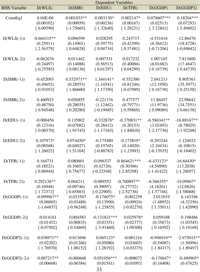
The remaining estimated results relating to the error correction terms, the lagged independent variables, are provided in table 5 & 6, accordingly. We divide the table into three panels – top, middle and bottom. The top panel explains the estimated coefficient, with standard errors ( ) and t-statistics [ ]. The middle panel provides the usual summary statistics for each of the six equations in the model, while the bottom gives the common summary measures for the full models.
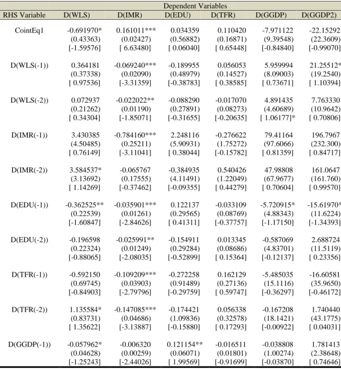
The adjustment coefficients for GGDP, GGDP2, TFR, and EDU are all statistically significant at the .01 level (at least) in table 5. Similarly, in table 6, IMR and other
endogenous variables are also significant at the same level. The explanation of significant coefficients means that these variables respond in the short-term to shocks to the dynamic
32
system that force it away from equilibrium (as embodied in the coefficient relation). It is also interesting to note that the absolute value of the growth domestic product per capital growth square (GGDP2) coefficient in both tables is substantially larger than from the other five variables; suggesting that GGDP2 reacts more quickly to movements away from equilibrium than the other five variables.
However, the adjustment coefficient for IMR is statistically insignificant in the case of Bangladesh (table 5). This shows that IMR does not react to deviations from the long-run equilibrium at all, which suggests that the IMR variable is "weakly endogenous". It is important to consider that this does not mean that IMR is completely exogenous. The long-run endogeneity makes firm the inclusion of the variable in the cointegration relation.
Second, a non-trivial number of the coefficients for the lagged variables have unexpected signs (e.g. positive coefficient for lagged IMR in the GDP equation in both tables) and/or are not statistically significant. On the basis of this calculation it can be
concluded that the model is fully over-parameterized. The construction of a succinct model is left as an assignment for future work. Nevertheless, the econometric output encourages many general modelling techniques and considers them as reasonable since they have statistically significant relationships and correct signs.
33
Bangladesh
Table 5. Estimation results for cointegrating equations and dependent variables coefficients Dependent Variables
RHS Variable D(WLS) D(IMR) D(EDU) D(TFR) D(GGDP) D(GGDP2) CointEq1 6.04E-06 -0.001033** -0.003130* 0.002147* 0.078607*** 0.18204*** (0.00102) (0.00059) (0.00236) (0.00167) (0.02513) (0.07293) [ 0.00590] [-1.75665] [-1.32640] [ 1.28231] [ 3.12841] [ 2.49602] D(WLS(-1)) 0.664315** 0.096599 0.028295 0.243717 -4.531616 -12.86476 (0.25911) (0.14901) (0.59775) (0.42399) (6.36412) (18.4728) [ 2.56379] [ 0.64828] [ 0.04734] [ 0.57481] [-0.71206] [-0.69642] D(WLS(-2)) -0.062676 0.011462 0.007331 0.017232 1.007165 7.813600 (0.24497) (0.14088) (0.56513) (0.40086) (6.01682) (17.4647) [-0.25585] [ 0.08136] [ 0.01297] [ 0.04299] [ 0.16739] [ 0.44739] D(IMR(-1)) -0.452093 0.532971** 1.344141* -0.552380 2.041213 8.905363 (0.49652) (0.28553) (1.14541) (0.81246) (12.1950) (35.3977) [-0.91053] [ 1.86660] [ 1.17350] [-0.67989] [ 0.16738] [ 0.25158] D(IMR(-2)) 0.460923 0.056855 -0.221376 0.477577 11.86457 22.98642 (0.48750) (0.28035) (1.12462) (0.79771) (11.9736) (34.7551) [ 0.94548] [ 0.20280] [-0.19685] [ 0.59869] [ 0.99089] [ 0.66138] D(EDU(-1)) -0.000456 0.135802 -0.332878* -0.370831** -6.586341** -16.88167** (0.12316) (0.07082) (0.28412) (0.20153) (3.02493) (8.78029) [-0.00370] [ 1.91743] [-1.17163] [-1.84010] [-2.17736] [-1.92268] D(EDU(-2)) 0.107973* 0.074450* -0.175480 -0.173819* -0.293244 -1.124032 (0.08568) (0.04927) (0.19765) (0.14020) (2.10434) (6.10815) [ 1.26022] [ 1.51104] [-0.88783] [-1.23983] [-0.13935] [-0.18402] D(TFR(-1)) 0.164731 0.080601 -0.096337 -0.864621*** -6.433123* -16.64430* (0.18521) (0.10651) (0.42726) (0.30306) (4.54890) (13.2038) [ 0.88944] [ 0.75677] [-0.22548] [-2.85298] [-1.41422] [-1.26057] D(TFR(-2)) 0.292136** 0.064211 -0.089552 -0.700897** -6.566355* -19.09867* (0.16948) (0.09746) (0.39097) (0.27732) (4.16261) (12.0826) [ 1.72372] [ 0.65883] [-0.22905] [-2.52736] [-1.57746] [-1.58068] D(GGDP(-1)) -0.099967** -0.033567 -0.176075* -0.002259 2.011019 6.143346 (0.06065) (0.03488) (0.13990) (0.09924) (1.48952) (4.32356) [-1.64837] [-0.96248] [-1.25855] [-0.02276] [ 1.35011] [ 1.42090] D(GGDP(-2)) -0.014161 0.004583 -0.131831*** 0.025978* 0.059188 0.198486 (0.01452) (0.00835) (0.03351) (0.02377) (0.35673) (1.03545) [-0.97502] [ 0.54869] [-3.93460] [ 1.09308] [ 0.16592] [ 0.19169] D(GGDP2(-1)) 0.038971** 0.013696 0.065123* -0.001216 -0.996919** -2.975015** (0.02202) (0.01266) (0.05080) (0.03603) (0.54087) (1.56996) [ 1.76970] [ 1.08152] [ 1.28192] [-0.03375] [-1.84317] [-1.89497] D(GGDP2(-2)) 0.007217** -0.000668 0.051056*** -0.008072 -0.170647* -0.490903* (0.00668) (0.00384) (0.01541) (0.01093) (0.16408) (0.47625)
34 [ 1.08034] [-0.17378] [ 3.31299] [-0.73842] [-1.04005] [-1.03076] C 0.015943* -0.015265** 0.054426** -0.090757*** 0.229252 0.362738 (0.01283) (0.00738) (0.02960) (0.02100) (0.31519) (0.91487) [ 1.24234] [-2.06857] [ 1.83849] [-4.32207] [ 0.72735] [ 0.39649] R-squared 0.557866 0.849327 0.817777 0.480437 0.785489 0.757004 Adj. R-squared 0.174683 0.718744 0.659850 0.030149 0.599580 0.546408 Sum sq. resids 0.000856 0.000283 0.004554 0.002291 0.516252 4.349604 S.E. equation 0.007553 0.004344 0.017425 0.012360 0.185518 0.538492 F-statistic 1.455873 6.504110 5.178197 1.066955 4.225115 3.594575 Log likelihood 110.0971 126.1419 85.85587 95.81611 17.26340 -13.63966 Akaike AIC -6.627389 -7.733926 -4.955577 -5.642490 -0.225062 1.906183 Schwarz SC -5.967315 -7.073852 -4.295503 -4.982416 0.435011 2.566257 Mean dependent 0.002298 -0.041927 0.007723 -0.035167 0.035783 0.099080 S.D. dependent 0.008314 0.008190 0.029877 0.012550 0.293175 0.799552 Determinant resid covariance (dof
adj.) 3.36E-23
Determinant resid covariance 6.44E-25 Log likelihood 560.7854 Akaike information criterion -32.46796 Schwarz criterion -28.22463
Note: t-statistics are in brackets. *, **, and *** refer to statistical significance at 0.10, 0.05, and 0.025 levels, respectively.
35
Pakistan
Table 6.Estimation results for cointegrating equations and dependent variables coefficients Dependent Variables
RHS Variable D(WLS) D(IMR) D(EDU) D(TFR) D(GGDP) D(GGDP2) CointEq1 -0.691970* 0.161011*** 0.034359 0.110420 -7.971122 -22.15292 (0.43363) (0.02427) (0.56882) (0.16871) (9.39548) (22.3609) [-1.59576] [ 6.63480] [ 0.06040] [ 0.65448] [-0.84840] [-0.99070] D(WLS(-1)) 0.364181 -0.069240*** -0.189955 0.056053 5.959994 21.25512* (0.37338) (0.02090) (0.48979) (0.14527) (8.09003) (19.2540) [ 0.97536] [-3.31359] [-0.38783] [ 0.38585] [ 0.73671] [ 1.10394] D(WLS(-2)) 0.072937 -0.022022** -0.088290 -0.017070 4.891435 7.763330 (0.21262) (0.01190) (0.27891) (0.08273) (4.60689) (10.9642) [ 0.34304] [-1.85071] [-0.31655] [-0.20635] [ 1.06177]* [ 0.70806] D(IMR(-1)) 3.430385 -0.784160*** 2.248116 -0.276622 79.41164 196.7967 (4.50485) (0.25211) (5.90931) (1.75272) (97.6066) (232.300) [ 0.76149] [-3.11041] [ 0.38044] [-0.15782] [ 0.81359] [ 0.84717] D(IMR(-2)) 3.584537* -0.065767 -0.384935 0.540426 47.98808 161.0647 (3.13692) (0.17555) (4.11491) (1.22049) (67.9677) (161.760) [ 1.14269] [-0.37462] [-0.09355] [ 0.44279] [ 0.70604] [ 0.99570] D(EDU(-1)) -0.362525** -0.035901*** 0.122137 -0.033109 -5.720915* -15.61970* (0.22539) (0.01261) (0.29565) (0.08769) (4.88343) (11.6224) [-1.60847] [-2.84626] [ 0.41311] [-0.37757] [-1.17150] [-1.34393] D(EDU(-2)) -0.196598 -0.025991** -0.154911 0.013345 -0.587069 2.688724 (0.22324) (0.01249) (0.29284) (0.08686) (4.83701) (11.5119) [-0.88065] [-2.08035] [-0.52899] [ 0.15364] [-0.12137] [ 0.23356] D(TFR(-1)) -0.592150 -0.109209*** -0.272258 0.162129 -5.485035 -16.60581 (0.69745) (0.03903) (0.91489) (0.27136) (15.1116) (35.9650) [-0.84903] [-2.79796] [-0.29759] [ 0.59747] [-0.36297] [-0.46172] D(TFR(-2)) 1.135584* -0.147085*** -0.174421 0.056338 -0.167208 1.740440 (0.83731) (0.04686) (1.09836) (0.32578) (18.1421) (43.1775) [ 1.35622] [-3.13887] [-0.15880] [ 0.17293] [-0.00922] [ 0.04031] D(GGDP(-1)) -0.057962* -0.006320 0.121154** -0.016511 -0.038808 1.781413 (0.04628) (0.00259) (0.06071) (0.01801) (1.00274) (2.38648) [-1.25243] [-2.44026] [ 1.99569] [-0.91699] [-0.03870] [ 0.74646]
36 D(GGDP(-2)) -0.064048* -0.004296* -0.010647 0.006024 0.310905 2.274415 (0.05419) (0.00303) (0.07108) (0.02108) (1.17411) (2.79434) [-1.18193] [-1.41666] [-0.14978] [ 0.28570] [ 0.26480] [ 0.81394] D(GGDP2(-1)) 0.024220* 0.003174*** -0.038887* 0.006054 -0.263061 -1.276449* (0.02046) (0.00114) (0.02683) (0.00796) (0.44324) (1.05488) [ 1.18398] [ 2.77219] [-1.44916] [ 0.76068] [-0.59350] [-1.21004] D(GGDP2(-2)) 0.036841** 0.002744*** 0.015355 -0.003905 -0.254432 -1.160013* (0.02145) (0.00120) (0.02814) (0.00835) (0.46483) (1.10628) [ 1.71728] [ 2.28509] [ 0.54562] [-0.46789] [-0.54736] [-1.04857] C 0.173637* -0.040791*** 0.046410 -0.014197 2.214876 6.206880* (0.11149) (0.00624) (0.14625) (0.04338) (2.41573) (5.74935) [ 1.55737] [-6.53748] [ 0.31733] [-0.32729] [ 0.91686] [ 1.07958] R-squared 0.729668 0.926961 0.563544 0.621965 0.429482 0.360844 Adj. R-squared 0.495380 0.863661 0.185282 0.294335 -0.064967 -0.193091 Sum sq. resids 0.012861 4.03E-05 0.022130 0.001947 6.037616 34.19837 S.E. equation 0.029281 0.001639 0.038410 0.011393 0.634435 1.509931 F-statistic 3.114409 14.64385 1.489823 1.898376 0.868608 0.651420 Log likelihood 70.80338 154.4119 62.93349 98.17894 -18.39456 -43.54001 Akaike AIC -3.917474 -9.683576 -3.374723 -5.805444 2.234108 3.968276 Schwarz SC -3.257401 -9.023503 -2.714650 -5.145370 2.894182 4.628350 Mean dependent 0.020999 -0.020795 0.010006 -0.023375 -0.027371 -0.081055 S.D. dependent 0.041220 0.004438 0.042554 0.013562 0.614779 1.382357 Determinant resid covariance (dof
adj.) 1.80E-19
Determinant resid covariance 3.45E-21 Log likelihood 436.2672 Akaike information criterion -23.88050 Schwarz criterion -19.63717
Note: t-statistics are in brackets. *, **, and *** refer to statistical significance at 0.10, 0.05, and 0.025 levels, respectively
37
Impulse response
This thesis uses impulse response analysis to estimate the impact of variables on one another to expose the long run dynamic interrelationship. The impulse response technique is a practical way to summarize the various complicated effects of variables.
Bangladesh
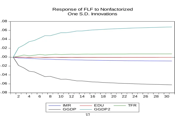
Figure 1shows the relationship of the five variables with their direction and magnitude in respect of their effect on women’s labour supply. The five variables are GGDP, GGDP2, IMR, TFR and EDU. The shock to GGDP on WLS is negative, although the square of the GGDP is positive. Moreover, the long-run association between TFR and EDU is positive with women’s labour supply, the effect of a shock to TFR and EDU on WLS increases their labour supply, while, the shock to IMR on WLS is negative; this means that for an increase in IMR (decline) WLS will decline (increase).
Figure 1 -.08 -.06 -.04 -.02 .00 .02 .04 .06 .08 2 4 6 8 10 12 14 16 18 20 22 24 26 28 30 IMR EDU TFR GGDP GGDP2 Response of FLF to Nonfactorized One S.D. Innovations
38
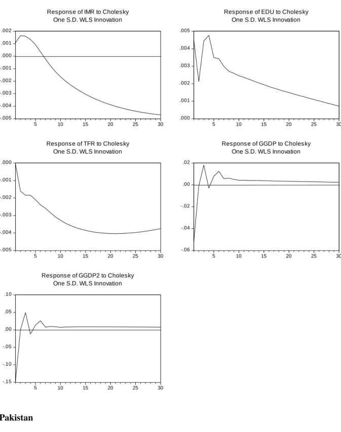
Figure 2 provides an overview of the shocks to WLS on IMR, EDU, TFR, GGDP and GGDP2 in Bangladesh. Almost all of the variables have fluctuating responses except EDU and TFR or are small in magnitude. The figure shows that the shock to WLS on IMR for the first seven years has a positive response, and then remains negative after that. This means that for the first seven years when WLS increases IMR also increases while after that period when WLS increases (decreases) IMR decreases (increases). The shock to WLS on EDU is continually positive while the shock to WLS on TFR remains negative throughout the period. This means that when WLS increases, EDU also increases and when WLS decreases TFR increases. The shocks to WLS on GGDP and GGDP2 are negative for the first three years then change to positive for about the next two years. It changes to negative for the fifth year and is then constantly positive throughout the period. This means that at some point, when WLS increases (decreases), GGDP and GGDP2increases (decreases).
39 -.005 -.004 -.003 -.002 -.001 .000 .001 .002 5 10 15 20 25 30
Response of IMR to Cholesky One S.D. WLS Innovation .000 .001 .002 .003 .004 .005 5 10 15 20 25 30
Response of EDU to Cholesky One S.D. WLS Innovation -.005 -.004 -.003 -.002 -.001 .000 5 10 15 20 25 30 Response of TFR to Cholesky One S.D. WLS Innovation -.06 -.04 -.02 .00 .02 5 10 15 20 25 30 Response of GGDP to Cholesky One S.D. WLS Innovation -.15 -.10 -.05 .00 .05 .10 5 10 15 20 25 30 Response of GGDP2 to Cholesky One S.D. WLS Innovation Pakistan
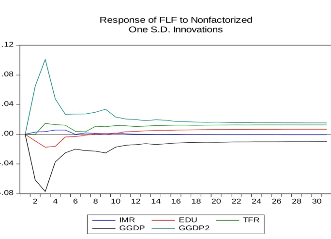
Figure 3 demonstrates that in the beginning, or sometime, IMR is positive when EDU is negative but as soon as EDU changes its quadrant and builds a positive relation with the WLS the IMR declines and has a negative relationship with WLS. Similarly, in Bangladesh the GGDP has a negative relation with WLS; however, the square of GGDP has a positive
40
relation, as in the case of Bangladesh. A shock to GGDP and GGDP2 on WLS will decrease its supply and increase its participation accordingly. The fertility rate has a positive
relationship with WLS. This means that the impact of a shock to fertility on WLS boosts supply. Figure 3 -.08 -.04 .00 .04 .08 .12 2 4 6 8 10 12 14 16 18 20 22 24 26 28 30 IMR EDU TFR GGDP GGDP2 Response of FLF to Nonfactorized One S.D. Innovations
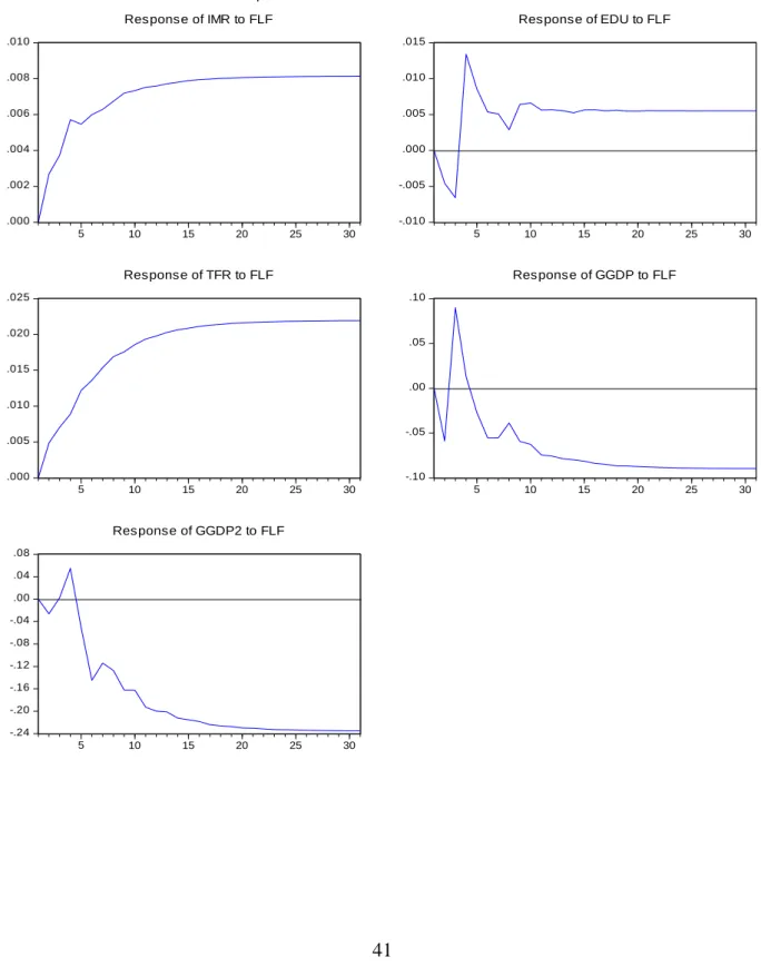
Figure 4 shows the shocks to WLS in Pakistan. The figures show that the shocks to WLS on IMR and TFR are positive. This means that if the rate of WLS increases, the rate of IMR and TFR also increases. While the shocks fluctuate for EDU, GGDP and GGDP2, the shock to WLS on EDU for the first three years is negative, which means that when WLS increases EDU decreases. The shock to WLS on EDU after three years is positive, which means that when WLS increases EDU also increases. A shock to WLS on GGDP and GGDP2 has a negative relationship in the first two years. After three years, the relationship changes to
41
positive. This means that in the early years, when WLS increases, GGDP and GGDP2 decrease. However, after the first five years the shock to WLS on GGDP and GGDP2 are inversed. This means that a decrease in WLS causes a decrease in GGDP and GGDP2.
Figure 4 .000 .002 .004 .006 .008 .010 5 10 15 20 25 30 Response of IMR to FLF -.010 -.005 .000 .005 .010 .015 5 10 15 20 25 30 Response of EDU to FLF .000 .005 .010 .015 .020 .025 5 10 15 20 25 30 Response of TFR to FLF -.10 -.05 .00 .05 .10 5 10 15 20 25 30 Response of GGDP to FLF -.24 -.20 -.16 -.12 -.08 -.04 .00 .04 .08 5 10 15 20 25 30 Response of GGDP2 to FLF
42
6. Conclusion
This thesis concerns the determinants of women’s labour supply in Bangladesh and Pakistan. All variables were entered in the estimated cointegration equation and considered as
endogenous in a dynamic system in the long run. Moreover, it is also noted that the estimated adjustment coefficients, such as GGDP, GGDP2, TFR and EDU, in the VEC model, show that, to some extent, they deviate from short run to long run equilibrium. Thus, this result suggests they should also be considered as endogenous variables in the short term. However, the results also show that the error correction parameter for the infant mortality rate is
insignificant. This indicates that the infant mortality rate does not adjust in the short-term to deviations from equilibrium. Therefore, the infant mortality rate is weakly exogenous. The cointegration equation confirms the U-shape hypothesis of women’s labour supply and economic development in both countries.
From the impulse response result, it is concluded that in the long run, the infant mortality rate, primary education, gross domestic product per capita growth and gross domestic product per capita growth square, have the expected sign for both countries. The comparison studies of Bangladesh and Pakistan show that a shock to GGDP and GGDP2 are negative and positive, respectively.
Secondly, it was expected that as the infant mortality rate and total fertility rate decrease, women will have more time to participate in the labour market. It is concluded that the infant mortality rate confirms the hypothesis that as the infant mortality rate decreases women’s labour supply increases. On the other hand, the total fertility rate has a positive
43
relationship with women’s labour supply. This means that as the total fertility rate increases, women’s labour supply increases.
Although primary education is noted as having a positive relationship with women’s labour supply in both countries, it can be concluded that the strength of a positive shock is relatively higher in the case of Bangladesh than Pakistan.
To achieve the goal, the thesis used a VECM analysis between the variables and women’s labour supply using the impulse response rate. The analysis is based on data from 1981 to 2011 from the World Data Bank.
44
Appendix A
Total Fertility Rate
Year Bangladesh Pakistan
1980 6.4 6.5 1985 5.5 6.4 1990 4.5 6 1995 3.7 5.4 2000 3.1 4.5 2005 2.6 3.8 2010 2.2 3.4
Infant Mortality Rate
Year Bangladesh Pakistan
1980 130.1 110.7 1985 113.2 104 1990 96.5 94.6 1995 78.8 86 2000 62 75.9 2005 49.1 67.8 2010 38.6 60.4
45
Appendix B
Definition of variables
Infant mortality rate
Infant mortality rate is the number of infants dying before reaching his/her one year age. It is calculated based on live births per 1,000 in a year.
Total fertility Rate
Total fertility rate is the number of children that would be born to a woman if she were to live to the end of her childbearing years and bear children in accordance with current age-specific fertility rates.
Primary Education
Primary education provides children with basic reading, writing, and mathematics skills together with an elementary understanding of such subjects as history, geography, natural sciences, social science, art, and music. Commonly, it takes about six years in the early education.
GGDP
46
Appendix C
Results for Bangladesh.
WLS IMR EDU TFR GGDP GGDP2 Mean 3.658049 4.300713 3.823239 1.308136 1.484966 2.380297 Median 3.659579 4.340865 3.860727 1.294633 1.605784 2.578675 Maximum 3.694613 4.868303 3.929666 1.856298 1.903315 3.622609 Minimum 3.612808 3.602777 3.609533 0.788457 -0.199498 0.039799 Std. Dev. 0.023575 0.393461 0.099245 0.341200 0.425232 0.925619 Sum 117.0576 137.6228 122.3437 41.86035 47.51893 76.16950 Sum Sq. Dev. 0.017229 4.799156 0.305337 3.608935 5.605480 26.55991 Observations 32 32 32 32 32 32
Results for Pakistan
WLS IMR EDU TFR GGDP GGDP2 Mean 2.655472 4.421458 3.622310 1.604984 1.502432 2.529096 Median 2.632954 4.439597 3.649637 1.667529 1.601645 2.565268 Maximum 3.042591 4.706824 3.787296 1.871802 2.323926 5.400633 Minimum 2.346602 4.080922 3.470604 1.193922 0.014293 0.000204 Std. Dev. 0.221470 0.196896 0.113234 0.236112 0.529680 1.368546 Sum 84.97509 141.4867 115.9139 51.35948 48.07783 80.93107 Sum Sq. Dev. 1.520519 1.201809 0.397479 1.728215 8.697393 58.06048 Observations 32 32 32 32 32 32
47
References
Acemoglu, D. (2007). Introduction to modern economic growth (1.1 ed.). New England, United States.: Massachusetts Institue of Tenhnology.
Achkah, C., Ahiadeke, C., & Fenny, A. P. (2009). Determinants of Female Labour Force
Participation in Ghana. Accra: Institute of Statistical, Social and Economic
Research,University of Ghana. Retrieved from
http://depot.gdnet.org/newkb/submissions/ISSER_Paper2_FINAL.pdf
Al-Qudsi, S. S. (1998). Labour participation of Arab women: estimates of the fertility to labour supply link. Applied Economics, 30(7), 931–941. doi:10.1080/000368498325363
Andersson, G. (2000). The impact of labour force particiation on childbearing behaviour: Pro-cyclical fertility in Sweden during the 1980s and the 1990s. European Journal of
Population, 16, 293–333.
Anker, R. (1983). Female Labour Force Participation in Developing Countries: A Critique of Current Definitions and Data Collection Methods. International Labour Review, 122, 709.
Ashraf, Q. H., Weil, D. N., & Wilde, J. (2013). The Effect of Fertility Reduction on Economic Growth. Population and Development Review, 39(1), 97–130. doi:10.1111/j.1728-4457.2013.00575.x
Asteriou, D., & Hall, S. G. (2007). Applied econometrics: A modern approach using Eviews
and Microsfit revised edition. New York: Palgrave macmillan.
Bangladesh Bureau of Statistics. (2011). Population and housing census 2011:
Socio-economimc and demographic report , volum 4. Dhaka: Bangladesh Bureau of
48
Beckar, G. S. (1965). A theory of the allocation of time. The Economic Journal, 75(299), 493–517.
Bloom, D. E., Canning, D., Fink, G., & Finlay, J. E. (2009). Fertility, female labor force participation, and the demographic dividend. Journal of Economic Growth, 14(2), 79– 101. doi:10.1007/s10887-009-9039-9
Doepke, M. (2004). Accounting for Fertility Decline during the Transition to Growth.
Journal of Economic Growth, 9(3), 347–383. doi:10.2307/40215875
Engle, R. ., & Yoo, B. . (1989). Cointegrated economic time series: A survey with new
results. Pennsylvania State-Department of Economic.
Fatima, A., & Sultana, H. (2009). Tracing out the U-shape relationship between female labor force participation rate and economic development for Pakistan. International Journal
of Social Economics, 36(1), 182–198.
Ganguli, I., Hausmann, R., & Viarengo, M. (2011). Closing the Gender Gap in Education:
Does it Foretell the Closing of the Employment, Marriage, and Motherhood Gaps?
CID Working Paper No 220, Centre for International Development at Harvard
University. Retrieved from
http://www.hks.harvard.edu/var/ezp_site/storage/fckeditor/file/pdfs/centers-programs/centers/cid/publications/faculty/wp/220.pdf
Goldin, C. (1994). The U-shaped female labour force function in economic development and
economic history. Cambridge: Department of Economics, Harvard University.
Greene, W. H. (2009). Econometric Analysis (Fifth.). New Delhi: Pearson.
Guillermo, C., & Quentin, W. (2003). Argentina’s crises and the poor, 1995-2002 (No. No. DARP 71). London: London School of Economics and Political Science.
49
Harmon, C., Oosterbeek, H., & Walker, I. (2003). The Returns to Education: Microeconomics. Journal of Economic Surveys, 17(2), 115–156. doi:10.1111/1467-6419.00191
Hondroyiannis, G., & Papapetrou, E. (2002). Demographic transition and economic growth: Empirical evidence from Greece. Journal of Population Economics, 15(2), 221–242. doi:10.1007/s001480100069
Jamaly, R., & Wickramanayake, E. (1996). Women Workers in the Garment Industry in Dhaka, Bangladesh. Development in Practice, 6(2), 156–161. doi:10.2307/4028981 Kelly, J. (1986). Women, History, and Theory: The Essays of Joan Kelly. University of
Chicago Press.
Kirk, D. (1996). Demographic transition theory. Population studies, 50(3), 361–387. doi:10.1080/0032472031000149536
Lewis, B. D. (2010). Demographic transition and economic growth in Indonesia. Bukit Timah Road: Lee Kuan Yew School of Public Policy.
Mazhar, N. (2013). Population labour force and employment. Pakistan: Ministry of Finance, Goverment of Pakistan. Retrieved from http://www.finance.gov.pk/survey_1112.html Mincer, J. (1962). Labor force participation of married women: A study of labor supply. In
Aspects of Labor Economics (National Bureau of Economic Research.). New Jersey:
Princeton University Press. Retrieved from http://www.nber.org/chapters/c0603 Mincer, J., & Polachek, S. (1974). Family investments in human capital: Earnings of women.
In Marriage, family, human capital and fertility (pp. 76–110). New York: UMI. Muhammad, A., & Fernando, R. (2010). Status of women and fertility in Pakistan. Canadian
Studies in Population, 37(1-2, Spring/Summer), 1–23.
50
Nguyen Thi Hong, T. (2009). The effects of fertility on female labor supply (Report). Kansas State University. Retrieved from http://krex.ksu.edu/dspace/handle/2097/1442
Phillips, P. C. B. (1987). Time Series Regression with a Unit Root. Econometrica, 55(2), 277–301. doi:10.2307/1913237
Richardson, D. K., Gray, J. E., Gortmaker, S. L., Goldmann, D. A., Pursley, D. M., & McCormick, M. C. (1998). Declining Severity Adjusted Mortality: Evidence of Improving Neonatal Intensive Care. Pediatrics, 102(4), 893–899.
Royalty, A. B. (1998). Job‐to‐Job and Job‐to‐Nonemployment Turnover by Gender and Education Level. Journal of Labor Economics, 16(2), 392–433. doi:10.1086/209894 Salehi-Isfahani, D., & Kamel, H. (2006). Demographic Swings and Early Childhood
Education in Iran (Working Paper). Virginia Polytechnic Institute and State
University, Department of Economics. Retrieved from
http://econpapers.repec.org/scripts/a/abstract.pf?f=/paper/vpiwpaper/e06-2.htm;terms=education+and+fertility
Singh, R. D. (1994). Fertility-Mortality Variations Across LDCs: Women’s Education, Labor Force Participation, and Contraceptive-Use. Kyklos, 47(2), 209–229. doi:10.1111/j.1467-6435.1994.tb02256.x
Snowdon, B., & Vane, H. . (2005). Modern macroeconomics:its origionals, development and
current state. Chelten ham: Edward Elgar.
Tamura, R. (2006). Human capital and economic development. Journal of Development
Economics, 79(1), 26–72. doi:10.1016/j.jdeveco.2004.12.003
Tansel, A. (2002). Economic Development and Female Labor Force Participation in Turkey:
Time-Series Evidence and Cross-Section Estimates (SSRN Scholarly Paper No. ID
301946). Rochester, NY: Social Science Research Network. Retrieved from http://papers.ssrn.com/abstract=301946