J
Ö N K Ö P I N GI
N T E R N A T I O N A LB
U S I N E S SS
C H O O LJönköping University
F D I a n d E c o n o m i c G r o w t h
A study of 7 transition economies of CEE and the Baltic States
Bachelor’s thesis within Economics Author: Felipe Domarchi
Daniel Nkengapa
Tutor: Börje Johansson, Professor
Tobias Dahlström, Ph.D. Candidate Jönköping January 2007
Bachelor’s Thesis in Economics
Title: FDI and Economic Growth
Author: Felipe Domarchi, Daniel Nkengapa
Tutor: Prof. Börje Johansson, Ph.D. Tobias Dahlström
Date: January 2007
Subject terms: Economic Growth, R&D, FDI, TFP growth
Abstract
This thesis analyses the effect of FDI induced technology transfer and spillover on economic growth in the CEE countries and the Baltic States. We develop a frame-work were FDI and R&D are seen as sources of technological progress (A). Transi-tion economies, due to the need to catch up quickly with more advanced economies, rely on FDI as a major channel through which they can tap the needed technology. Whether or not technology spills over to the entire economy depends on the ability of the countries to diffuse the advanced technology transferred by FDI. We test us-ing panel data analysis, if FDI alone can spur growth or whether the FDI induced technology spillover effect is enhanced by the level of R&D.
Empirical evidence is found that FDI and R&D as an interaction term have helped the CEE countries and the Baltic States to accelerate growth by modernizing the economy through an upgrading process.
Table of Contents
1
Introduction... 1
1.1 Problem ... 1 1.2 Previous Research ... 2 1.3 Purpose ... 2 1.4 Research Strategy... 2 1.5 Outline ... 32
Theoretical Framework... 4
2.1 The twin role of FDI in host countries ... 4
2.2 Economic Growth ... 5
2.2.1 Growth Accounting... 5
2.3 FDI as an investment enhancer... 6
2.4 FDI as a vehicle of technology transferred ... 6
2.4.1 FDI and technological development... 7
3
Descriptive Statistics... 9
3.1 Magnitude and Trend of FDI... 9
3.2 Magnitude and trend of GDP ... 11
3.3 Magnitude and trend of R&D ... 12
4
Empirical Framework... 14
4.1 Time period studied and data selection ... 14
4.2 Model specification ... 14 4.2.1 First model: ... 15 4.2.2 Second model: ... 16 4.3 Econometric results ... 16
5
Analysis... 21
6
Conclusion ... 23
6.1 Further Studies ... 237
References ... 24
Appendix I... 26
Appendix II... 26
Appendix III... 26
Figures
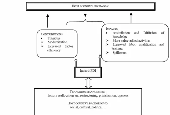
Figure 1 Host economy upgrading from FDI inflows ... 4
Figure 2 NetFDI per capita dollars for the CEE Countries and Baltic States 1992-2004... 10
Figure 3 GDP per capita in dollars for the CEE countries and Baltic States 1992-2004... 12
Figure 4 R&D per capita in dollars for the CEE countries and Baltic States 1992-2004... 13
Tables
Table 1 Cumulative FDI inflows, 1992-2004, GDP per capita in 2004, Cumulative R&D per capita 1992-2004 ... 9Table 2 Econometric results data... 17
Table 3 Econometric results data... 19
Table 4 Regression A Normality test. (Jarque-Bera)... 26
Table 5 Regression B Normality test. (Jarque-Bera)... 26
Table 6 Regression C Normality test. (Jarque-Bera) ... 26
Table 7 Regression D Normality test. (Jarque-Bera) ... 26
Table 8 Regression E Normality test. (Jarque-Bera)... 26
Table 9 Regression F Normality test. (Jarque-Bera) ... 26
Table 10 Regression G Normality test. (Jarque-Bera) ... 26
Table 11 Regression H Normality test. (Jarque-Bera) ... 26
Table 12 Normalized econometric results ... 26
Introduction
1
Introduction
One of the main economic policies that economists, researchers and governments in both transi-tional and less developed nations have often encouraged, from time immemorial, has been the is-sue of achieving high rates of economic growth. This is because it leads to high incomes, in-creased employment and availability of varieties which enhances living standards. Economists have often tried to unveil the main factors accounting for the growth in output on which living standards depend. Solow (1957) shows that the growth in output is due to capital accumulation and technological progress, but leaves the latter as an unexplained residual. With the diminishing marginal product of capital coupled with the exogenous technological progress, the economy reaches its long run level of output called the steady state. At this point, the economy ceases to grow because the amount of new capital produced is just enough to replace the capital lost due to depreciation. This makes the model inappropriate to explain the differences in long run growth across countries. It was thanks to the endogenous growth model starting with Romer (1986, 1990b), Lucas (1988), Grossman and Helpman (1991) that a glaring explanation to the impor-tance of knowledge as an endogenous determinant of growth was envisaged.
1.1
Problem
Long run growth depends on productivity and productivity depends on the level of technological progress. When the level technological progress is high, productivity increases since factors of production become more efficient, and the growth rate of output is increased. This has been the main motivation why companies and government encure huge expenses on education, on-the job training and research and development (R&D) aiming at upgrading the level of domestic knowl-edge to enhance the efficiency of factor inputs. Apart from the level of domestic knowlknowl-edge, for-eign knowledge also becomes available in the country through Forfor-eign Direct Investment (FDI). Gaining access to modern technology to augment the level of domestic technology thus provides a rational for attracting FDI. Thus, making the assertion that growth in transitional economies can be partly explained by a catch-up process in the level of technology from advance economies can hardly be denied. Countries seek FDI to provide them with inputs needed to grow and de-velop and in this vein tilt their national policies towards attracting more FDI. Alfaro, Areendam, Kalemli-Ozcan and Sayek (2004) postulates that the motive for attracting FDI stems from the belief that FDI brings several positive effects such as productivity gains, technology transfer, the introduction of new processes, managerial skills, and know-how in the domestic markets. The magnitude of the effect of advanced technology on economic growth depends on the extent to which the host country is able to absorb the technology. When the absorptive capacity is high the more technology spills over to the entire economy and the greater the effect on growth. The World Bank’s (2001) edition of global development and finance elucidates the role of absorptive capacities and the success of FDI and demonstrates how some countries with low absorptive ca-pacities such as Morocco and Uruguay failed to reap spillovers while others like Malaysia and Taiwan fared well with high absorptive capacities.
Developing and transitional economies often lack the needed capital and advanced technology hence rely on foreign sources to add to their existing resources. FDI has therefore been seen as a major channel through which these countries tap the needed capital and technology with the view that the technology would spillover to domestic firms thereby enhancing the overall level of pro-ductivity. The case of the transitional economies of Eastern Europe began with a structural change in both their political and economic institutions. After the 1990s the economies of East-ern Europe moved from a planned economy to a market economic system were market forces became the main determinant of the production and allocation of the national cake. The move-ment from the planned economy to market system coupled with an attractive package of invest-ment climate marked the beginning of massive FDI inflows into this region.
1.2
Previous Research
The issue of FDI and economic growth has been investigated by several researchers, but most of these studies have often focused more on the role of FDI in augmenting the level of domestic capital thereby accelerating growth. Studies on the role of FDI in transferring technology and the possibility of spillover to the domestic economy have been elusive, thus providing a strong moti-vation for this study. From a theoretical point of view, existing evidence show that FDI contrib-utes to growth but the extent of this contribution depends on the host country’s ability to reap the fruits of FDI. Borensztein, De Gregorio and Lee (1998) postulates that FDI would have a greater impact on growth when the labour force in the host country is educated enough to be able to absorb the spillover effects from FDI. They used human capital as a proxy for absorptive capacity and stress that the higher productivity of FDI only holds when there is a minimum threshold stock of human capital in the host country to diffuse the advanced technology from FDI. When MNEs introduce new knowledge, domestic firms may benefit from it through a spillover process. When the absorptive capacity in the domestic economy is high the rate of tech-nology diffusion is accelerated. Alfaro et al. (2004) also assert that FDI conveys greater knowl-edge spillover but the ability of a country to take advantage of this externality may be limited by local conditions. They also used financial institutions as a proxy for local conditions and argue that the lack of well developed financial institutions can limit the country’s ability to take advan-tage of potential FDI spillovers.
Our research takes its cue from the role of R&D which we use as a proxy for absorptive capacity and argue that the higher the level of R&D, the greater the rate of technology diffusion through knowledge spillover.
Transition Economies of Eastern Europe have been able to attract substantial FDI inflows since the early 1990. In 1995 FDI inflows exceeded $14bln and reached $21bln in 2001. Between 1995 and 2001 the total inward FDI stock increased four-fold, from $40bln to $160bln (UN 2003p.1). Within the region, some countries have grown more than others in the same time period receiv-ing almost the same amount of FDI per capita inflows. In a sense it is important and challengreceiv-ing to see to what extent the FDI inflows have been able to influence the host country’s economy so much that it has created more economic growth. This study does not argue that economic growth is dependent only on FDI inflows. While it is acknowledged that several other factors af-fect economic growth, the focus here is to uncover the role of FDI in transferring technology and the possibility of technology spillover to the domestic economy thereby enhancing economic growth.
1.3
Purpose
The purpose of this thesis is to analyze whether the technological spillover effect of FDI on eco-nomic growth in the CEE countries and the Baltic States is conditioned on the level of domestic R&D or not. Given that FDI and R&D are both sources of technological progress, it is interest-ing to investigate if FDI alone can spur growth in these economies or whether the extent to which FDI induces spillovers depends on the absorptive capacity, proxied by the level of R&D in these economies.
1.4
Research Strategy
Data on net FDI, GDP, gross capital formation and R&D, was collected from 1990 to 2004. The following countries considered in our analyses include; Poland, Czech Republic, Hungary, Slova-kia, Slovenia, Latvia and Lithuania.
Introduction
The influence of FDI on growth can be viewed from two angles. Firstly, as capital augmenting, thus total investment in a country consist of both domestic and foreign investment. Therefore, FDI has the potential to increase the total amount of investment which influences economic growth. Thus we will test this assumption with regard to the gross capital formation with respect to GDP and FDI with respect to GDP.
Secondly, the technological transfer and spillover effect is much more difficult to spot, especially the latter, since we cannot measure technological transfer and the spillover effect in quantitative terms. Krugman (1991) expresses it as “it leaves no paper trail” and hence one should focus more on the variables that are possible to quantify and see the result from. Thus we would analyze the role of FDI in transferring technology and the possibility that this technology would spillover by looking at the variables we can quantify, this would be FDI inflows and the positive change of GDP level and economic growth. We would use FDI and R&D as an interaction term to test if R&D enhances the impact of technology transfer on economic growth.
1.5
Outline
The rest of this thesis is organized as follows. Section 2 presents the growth accounting equation which serves as the main theoretical framework on which the econometric model is developed followed by some literature on knowledge spillover. Emphasis is placed on the increasing impor-tance of FDI in transferring advanced technology and the possibility of spillover to the entire economy. Trends in FDI and GDP, with possible justifications, within the eastern European re-gion are discussed in section 3. The empirical model and results are presented in section 4. The analysis is dealt in section 5 while conclusion and suggestions for further studies are presented in section 6.
2
Theoretical Framework
This section is divided into four subsections. The first subsection presents a vivid picture of twin role of FDI in host countries. In the second we present the growth accounting equation were we emphasize how changes in technology (A) can drive growth. In the third we discuss FDI as a capital augmenting and investment-enhancing tool. In the fourth, we discuss FDI as a channel of technology transfer and how it can spillover to the host economy.
2.1
The twin role of FDI in host countries
Figure 1 below captures the role of FDI in upgrading the economy through its contribution and impacts. The FDI contributions captures all the transfers from the MNE to the host country and includes technology, capital, expertise., know-how and organisational practices. These transfers are made to modernise and adapt local factors to foreign investors criteria and managerial frame-work (Fabry, 2000). This result in increasing factor efficiency and a modernisation of the econ-omy. The impact of FDI in the host country is concerned with the assimilation and diffussion of knowledge. This is more of a qualitative aspect. FDI brings in advanced technology that leads to increasing returns in domestic production and increases the value-added content of FDI-related production. The greatest and more long term impact of FDI is that of spillovers which occurs when the the advanced technology from FDI is able to trickle down to the entire economy. FDI induces more spillovers when the host country developes its institutions in such a way that they are able to absorb the technology from FDI. The movement from a command to a market sys-tem led to a restructuring of the CEE countries and the Baltic economies characterised with pri-vatisation and openess to the rest of the world. With the massive inflow of FDI coupled with its contribution and impacts led to an upgrading of these economies.
Figure 1 Host economy upgrading from FDI inflows
Theoretical Framework
2.2
Economic Growth
2.2.1 Growth Accounting
The standard growth accounting equation approach of Solow (1957) can be used to capture the factors that account for the growth in total output. The Solow growth accounting framework shows that the growth rate of total output depends on the growth rate of capital and labour weighted by their shares of income plus the level of technological progress.
*
(
) *
Y
K
N
A
1
Y
θ
K
θ
N
A
∆
∆
∆
∆
=
+
−
+
(2.1)Where Y =GDP, θ and (1-θ) are equal to capital and labour share of income respectively, K is the amount of capital, N is equal to labour force, and A is the level of technology.
The growth accounting equation, presented in 2.1 above, summaries the contribution of growth of inputs and improved productivity to the growth in output. Capital and labour each contribute an amount equal to the share of their income multiplied by their growth rates. The total factor productivity (TFP) is the amount by which output would increase when all inputs remain un-changed. This results from improvement in the method of production which increases the effi-ciency of factor inputs hence more output is produced. Solow found that the growth in output outpaced the weighted average increase in capital and labour inputs. This difference has often been termed the Solow residual. Thus, if we know the proportional growth rates of output, the labour force and the capital stock, then we can use the growth accounting equation to calculate the growth rate of technological progress.
The level of technology in an economy can be decomposed into two main parts. First, it depends on the level of human capital and R&D. With R&D expenditures, the potential for new knowl-edge emerges thus creating fertile ground for new inventions and innovations. Hall and Taylor (1997) support this assertion by postulating that the long run growth of technology is dependent on the number of workers in the technology production and the number of people doing re-search. An increase in the number of workers will increase the growth rate of technology ∆A/A. Since ∆A/A appears in the growth accounting equation a permanent increase in research will cause a permanent increase in the rate of growth. Second, apart from the level of knowledge cre-ated within an economy, foreign knowledge becomes available to the economy through FDI. FDI according to Mansfield and Romeo (1980) has therefore been seen as the cheapest means of transferring technology, as the recipient firms do not need to finance the acquisition of new technology and the transfer of technology is faster then licensing and international trade. Since it has a direct effect on the efficiency of firms, its has the possibility of creating spillover to other firms
From equation 2.1 above, an interesting question to ask is what determines the rate of technical progress (A)? The assumption in this thesis is that the rate of technical progress (A) depends on the amount of R&D expenditure and the technological inflow from FDI. With R&D expendi-tures, the potential for new knowledge emerges thus creating a fertile ground for new inventions and discoveries. Since the contribution of new knowledge is only partially captured by the creator there can be substantial external benefits through knowledge spillover to other firms. Mansfield and Romeo (1980) present a similar argument. They assert that FDI transfers knowledge more quickly than licensing and international trade and that since it has a direct effect on the efficiency of firms, it has the potential to create spillover to the overall economy. It should be noted that the extern to which knowledge spills over to the economy depends on the absorptive capacity of the economy. The absorptive capacity in this paper is proxied the level of R&D expenditures. The higher level of R&D expenditure the higher the absorptive capacity and the more the
multi-plier effect of technology spillover. Cohen and Levinthal (1989) support this hypothesis by postu-lating that R&D has two complementary effects on the level of productivity growth. First, they presented the innovative effect resulting from the direct expansion of firms technology level by new innovations through R&D. Secondly, R&D increases firms absorptive capacity-ability to identify, assimilate and exploit outside knowledge ,which the term learning or absorptive effect. This is consistent with our assumption, theoretically, that the higher the R&D expenditure the higher the absorptive capacity and greater the growth enhancing ability of FDI through knowl-edge spillover. It is on this premise that we interact FDI and R&D in the regression model.
2.3
FDI as an investment enhancer
One channel through which FDI impact growth is the possibility of bringing additional capital to the host country. In addition to the knowledge capital, FDI can also generate an inflow of physi-cal and human capital to the host country (Johnson, 2005).
The total investments in a country, measured by the gross capital formation, consist of both do-mestic and foreign investment. Standard economic growth theory asserts that an increase in the level of total investment would have a positive effect on growth. Therefore an increase in the level of FDI would lead to an increase in the gross capital formation and in turn spur growth. It is important to note that an inflow of capital is more evident in the case of Greenfield invest-ment rather than Brownfield investinvest-ment. The former brings in greater capital because it involves the establishment of a new facility while the latter mainly involves a change in ownership hence less additional capital is added (Johnson, 2005). Caution must also be drawn to the fact that the effect of FDI on economic growth depends on whether FDI is complementing or substituting domestic investment. When FDI complement domestic investment, for example supplying in-puts, crowding in occurs and impacts growth positively. Through competition in the host coun-try, FDI may crowd out domestic investment and negatively affect growth.
The impact of FDI on growth through its enhancement of domestic capital only occurs in the short run due to diminishing returns to capital. Economic theory suggests that long run growth depends on the rate of technological progress. Easterly and Levein (2001) confirmed this hy-pothesis by asserting that physical capital is relatively unimportant in explaining long run growth since most of the cross-country differences in growth is due to technical progress.
2.4
FDI as a vehicle of technology transferred
It has been widely argued through literature about the importance of FDI as a vehicle for trans-ferring technology to less developed economies. It is first important to give the attributes of technology in order to fully explain how changes in technology drive economic growth. Technol-ogy can neither be treated as a public nor as a competitive good, since it has the characteristics of both (Romer, 1990a).
It is partly excludable to treat technology as a pure public good since companies can and will try to keep the new technology they have out of the hands of competitors and the rest of the econ-omy. The fact that MNEs prefer to internalize international production rather than to give a li-cense to a domestic firm also supports this claim (Romer, 1990a). For countries, it can also be the case that they encourage this kind of behaviour since the social benefits of introducing a new technology are greater than the private benefits. Many countries give patents to firms with new technology aiming to motivate and strengthen the institutional framework surrounding invest-ments in R&D, otherwise few companies would engage in these activities. Without this protec-tion the country would be in a situaprotec-tion where little or no technological development would oc-cur. The underlying assumption is that the benefits to the society are higher than the
private-Theoretical Framework
benefits, encouraging the government to make incentives for companies to further invest in R&D (Romer, 1990a).
On the other hand, the fact that technology is partly excludable explains the technology gaps that are realized between companies and across countries. But the fact that technology as a good is not completely excludable is very important. As if it was completely excludable spillovers would not appear, and hence the technological progress by a firm would not be spread to the host economy.
Another characteristic of technology is that it is non-rival, meaning that there is no additional cost for a firm to employ an already developed technology. This implies that new technology when introduced and spread in the host economy will be available to an infinite number of eco-nomic agents that can use it without any additional cost. So the effects will be, when spread, a benefit for the host economy (Romer, 1990a).
2.4.1 FDI and technological development
MNEs are by definition assumed to have a high level of technology, and they are the firms that primarily carry out FDI. It is this advanced technology that enables MNEs to overcome the dis-advantages in a foreign location. The transfer of technology to the host economy is addressed to be in different stages (Uppenberg & Reiss, 2004).
Firms acquired by an MNE will have a more advanced technology than the surrounding econ-omy, concluding that the average level of technology and productivity in the country will be higher.
The probably more disputed and also most important contribution is the technological spillovers. The potential for technology spillovers from FDI is the positive externality of FDI that host countries hope to benefit from (Johnson, 2005). According to Blomstrom and Kokko (2003), the possibility of technology spillovers is one of the major reasons that host country governments try to attract more FDI. Technology does spillover, voluntary or involuntary, and usually in through backward and forward linkages:
• Intra-industry spillovers: productivity spillovers to companies within the same industry as the FDI. To follow the arguments of Romer (1990a) and Borensztein et al. (1998), this is driven by the production of new intermediate capital goods, which implies that the higher the technology in the intermediate goods the higher the technology is needed by the final producer of the good, and the final producer will have to adopt the new technology themselves. This situation is known as forward linkages. Backward linkages occurs when the MNE buys intermediate inputs from the local firms and in this case it is in the MNEs interest to voluntarily pass on the knowledge to the local firms to have high quality inputs (Javorcik, 2004) In addition, the competitors will have to become more productive to stay competitive; hence they will invest in the new technology as well in order to survive. • Inter-industry spillovers: productivity to other industries than where the FDI is active.
This is mainly driven by the overall rise in the level of knowledge of production in the economy and this will be enjoyed by all firms not only the ones in the specific production undertaken by the FDI-owned firms (Uppenberg & Reiss, 2004).
Technology spillovers can be observed also as workers don't tend to stay in the same firm throughout their lifetime. This suggests that knowledge will be transferred between companies. Although it is known that companies try to avoid this by offering loyalty-contracts to their work-ers, it is not fully possible to stop the spillover effect due to labour transfers. Another possible
spillover of technology is the "spread by air", workers socialise with other workers of other com-panies after working hours, and to prevent them to talk about work related issues including the technology used is almost impossible (Krugman, 1990). Even thought the spillover theory by Marshall (1920) has been widely criticised, because it is impossible to measure the effects in quan-titative terms, it is therefore really difficult to address its full effects on economic growth. We do acknowledge this criticism but it is to our belief that technological spillovers are important for economic development and for the aim of this thesis.
Descriptive Statistics
3
Descriptive Statistics
In this section, we are going to illustrate, using figures, tables and graphs, the magnitude and trend of FDI, and GDP within the Eastern European region and Baltic States. Variations in both the magnitude and trend would be accounted for.
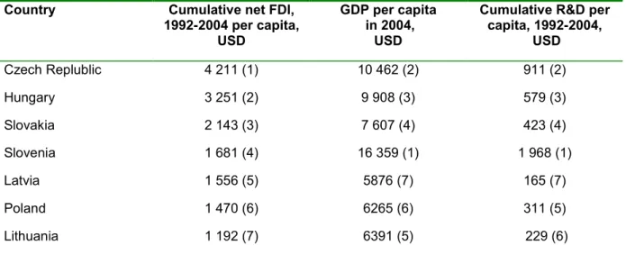
Table 1 Cumulative FDI inflows, 1992-2004, GDP per capita in 2004, Cumulative R&D per cap-ita 1992-2004
Country Cumulative net FDI,
1992-2004 per capita, USD
GDP per capita in 2004,
USD
Cumulative R&D per capita, 1992-2004, USD Czech Replublic 4 211 (1) 10 462 (2) 911 (2) Hungary 3 251 (2) 9 908 (3) 579 (3) Slovakia 2 143 (3) 7 607 (4) 423 (4) Slovenia 1 681 (4) 16 359 (1) 1 968 (1) Latvia 1 556 (5) 5876 (7) 165 (7) Poland 1 470 (6) 6265 (6) 311 (5) Lithuania 1 192 (7) 6391 (5) 229 (6)
Source: the writers processing of data from ERBD (2004) and UNCTAD (2005)
In Table 1 above, it is possible to see a pattern. The countries that have cumulated higher amount of FDI per capita during the transition between the years 1992-2004, also have recorded the highest GDP per capita at the end of the period. It is also possible to see from table 1, that coun-tries that engaged in R&D activities have higher GDP per capita at the end of the period studied. GDP per capita measures how “rich” a country is and this is important for our study, since the demand for high quality goods in these economies would attract high quality FDI.
3.1
Magnitude and Trend of FDI
FDI can be vital in helping transition economies to boost their level of output thereby catching-up with other regions of the world. FDI brings in new ideas, production techniques and man-agement practises that can help the economy upgrade through a spillover process.
Prior to the transition era, around the 90s, central and eastern European countries did not receive much FDI inflows. According to UNCTAD (2002 p.7) this region only accounted for 0.1% of global FDI inflows between 1986 and 1990. Until 1990 total FDI inflows were less than $1bln. The restructuring of the economy prompted a relative investment boom thus making the area more attractive to MNEs. In 1995 FDI inflows exceeded $14bln and reached $21bln in 2001. Be-tween 1995 and 2001 the total inward FDI stock increased four-fold, from $40bln to $160bln (UN 2003p.1). Therefore, the transition together with its characteristics in this region attracted the massive inflow of FDI. As a result the transition economies captured about 13.3% of FDI in developing countries, up from 11.2% in 2000 (UNCTAD, 2002).
However, the flow of FDI has not been evenly distributed across the countries as can be ob-served from table 1 above. From the table we can see that Czech Republic recorded the highest cumulative net FDI stock for the period 1992-2004. Hungary, Slovakia and Slovenia came next in
descending order of magnitude. Lithuania, Poland and Latvia achieved the lowest cumulative net FDI stock during the period, respectively.
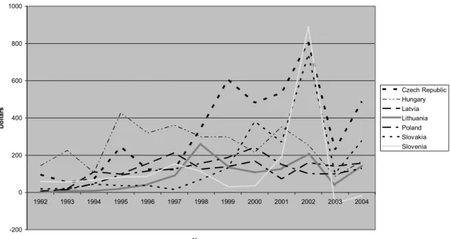
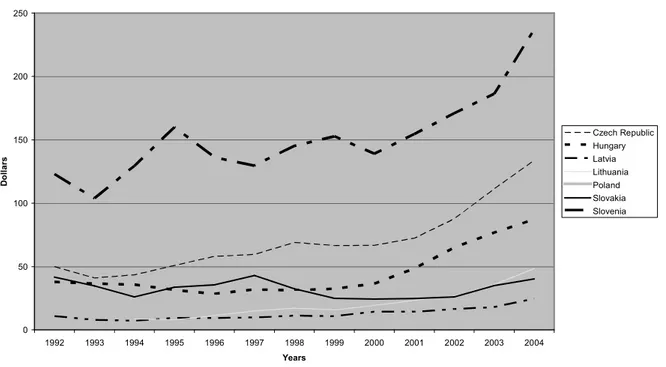
Figure 2 shows the trend of net FDI in the different countries of our sample. As shown on the graph, the trend has been undulating for all countries. Some countries, as discussed below, have received more than others within the period. A number of reasons can be used to explain these differences. The degree of privatisation, progress made by various states in terms of transition to market economy and prospects of EU accession justifies this variation. Hungary was the lead re-cipient in the early period of the transition because she opened more quickly to foreign investors. This was owed to the fact that Hungary started privatisation early by experiments in joint ven-tures during the soviet period. Therefore, there were more opportunities there. With the launch-ing of privatisation by other countries such as Czech Republic and Slovenia substantial flows of FDI was evident with Czech Republic on the lead. In short, the Czech Republic, Hungary and Slovenia offered investors access to relatively large, fast growing and stable markets and were the first to begin membership negotiations with the EU. With the completion of their privatisation programmes other countries emerged on the frontier. This reason justifies the decline in the net FDI per capita in Hungary. As evident from figure 2, Slovenia recorded $889 net FDI per capita, Czech Republic recorded $808 and Slovakia recorded $742 net FDI per capita in 2002. The Czech Republic is one of the most successful transition economy in attracting FDI in Eastern Europe. According to the European Union’s Official statistics Office Eurostats, the Czech Re-public has enjoyed a significant inflow of FDI than any other new EU member state in the year to date. FDI inflows increased from 5.2 billion € in 2003 to 8.8 billion € in 2004. This has been thanks to an attractive package of investments incentive by the government, its geographical proximity, a well educated and cheap labour force and the lordable efforts of the investment promotion agency. The introduction of investment incentives in 1998 has stimulated a massive inflow of FDI into both Greenfield and Brown field projects and since 1993 nearly €40bn in FDI has been recorded. More than 99000 Czech firms are now supported by foreign capital.
Net FDI /capita
-200 0 200 400 600 800 1000 1992 1993 1994 1995 1996 1997 1998 1999 2000 2001 2002 2003 2004 Years D o ll a rs Czech Republic Hungary Latvia Lithuania Poland Slovakia Slovenia
Figure 2 NetFDI per capita dollars for the CEE Countries and Baltic States 1992-2004
Descriptive Statistics
3.2
Magnitude and trend of GDP
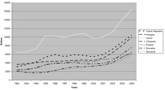
Gross domestic product (GDP) is the variable that is often used to measure the level of eco-nomic growth in an economy. GDP is defined as the value of all goods and services produced within an economy over a given period of time. Economic growth occurs when the value of real GDP increases over time. Theories of economic growth emphasize the importance of interna-tional linkages in accelerating the productive performance of individual nations. Before the transi-tion, the economies of Eastern Europe suffered from a prolonged stagnation or recession in the level of economic activities. The ownership, control and allocation of resources was under the auspices of the government and this lead to low output due to limited competition and little or no incentive for hard work. This lead to low rate of economic growth in the region. The 90s saw a transformation of the economic system from a planned economy to a market system aiming at boosting output, through privatization, stabilization and increased competition, thus enhancing living standards. This period marked the beginning of the massive inflow of FDI because coun-tries saw FDI as a channel through which they can tape the needed capital and technology neces-sary for growth. At the beginning of the transition, as seen on figure 3, the level of output per capita was low for all the countries. This was due to reasons such as disorganization of the for-mer institutions; huge amount of obsolete fixed capital and the fact that some workers went re-dundant as their skills were no longer needed. As time went on, these countries became more at-tractive to MNEs and GDP per capita started to rise for all countries. The prospect of EU ace-sion helped the countries to achieved increasing GDP per capita, through transparency of the in-titutions and the macro stability that these coutries had to ensure to meet the EU standard. From table 1 it is evident that Slovenia had the highest GDP per capita in 2004, at the end of the period studied, followed by Czech Republic and Hungary in descending order, respectively. From the same table, Lithuania, Poland and Latvia recorded the lowest GDP per capita in descending or-der of magnitude, respectively. According to the European Commission, Slovenia is the richest among the accession countries as its GDP per capita stood at 74 percent of the EU average in 2002, in purchasing power standards. Czech Republic is the next with GDP per capita approach-ing 60 percent of EU average. Poland is the poorest country in the sample with GDP per capita around 40 percent of EU average.
GDP/capita 0 2000 4000 6000 8000 10000 12000 14000 16000 18000 1992 1993 1994 1995 1996 1997 1998 1999 2000 2001 2002 2003 2004 Years D o ll a rs Czech Republic Hungary Latvia Lithuania Poland Slovakia Slovenia
Figure 3 GDP per capita in dollars for the CEE countries and Baltic States 1992-2004
Source: the writers processing data from UNCTAD (2005)
3.3
Magnitude and trend of R&D
In our study, R&D spending per capita is important since we use it as a proxy for ‘domestic knowledge’ or absorptive capacity. From table 1, it is possible to spot a trend. Countries such as Slovenia, Czech Republic and Hungary respectively, have spent more in R&D per capita terms and have achieved the highest GDP per capita at the end of the period studied. It is also possible to see from table 1 that countries such as Lithuania, Poland and Latvia have had low R&D per capita spending in cumulative terms during the period 1992-2004 also achieved the lowest GDP per capita at the end of this period, 2004. From figure 4 it is possible to see that the trend has been undulating, despite this undulating trend, Slovenia still stands out to have the highest ex-penditure on R&D.
Descriptive Statistics R&D/capita 0 50 100 150 200 250 1992 1993 1994 1995 1996 1997 1998 1999 2000 2001 2002 2003 2004 Years D o ll a rs Czech Republic Hungary Latvia Lithuania Poland Slovakia Slovenia
Figure 4 R&D per capita in dollars for the CEE countries and Baltic States 1992-2004
Source: the writers processing data from Eurostat (2006).
From the discussion above it has been shown that GDP per capita was high for some countries and low for other countries. FDI and R&D, as presented in the theoretical framework (in equa-tion 2.1), are important sources of technological progress on which economic growth depends. Therefore it is interesting to see if the differences in GDP per capita in these countries was due to the spillover effect of FDI and the absorptive capacity proxied by the level of R&D. The fol-lowing section provides an econometric analysis to see if the differences in GDP per capita was due to spillovers from FDI and absorptive capacity, proxied by R&D spending.
4
Empirical Framework
In the theoretical framework section we found evidence for the following variables to be included in the empirical analysis, GDP, Gross Fixed Capital Formation, R&D, R&D and FDI as an interaction term. With this in mind, we will analyze through econometric analysis, if these variables can shed light on the technological spillover ef-fect of FDI on economic growth.
4.1
Time period studied and data selection
The time period chosen for this study is from 1992 to 2004. This period is of much importance because it has been during these years that the transition economies of Eastern Europe have re-ceived substantial inflows of FDI and with it a great modernization of the industry has follow in these economies. The time period aimed at, from the beginning, was from 1990 to 2004 but it was not possible to retrieve all the necessary data for that period.
The sample of countries chosen for the analysis consists of 7 central European transition econo-mies including the Baltic States excluding Estonia and excluding most of the Balkan countries with the exception of Slovenia. The motive of using this sample of countries is that they are part of the 10 newly ascendant countries of the EU. And since the EU through the Eurostat webpage provides reliable data we had to use these countries.
GDP were obtained both in totals and in per capita terms. GFCF was obtained as percentage of the total GDP of the given year and thus a calculation was needed to convert it to quantitative terms. We subtracted net FDI from GFCF to have the domestic investments. Net FDI were found on EBRD transition report -infrastructure 2004. Due to the fact that we are interested in capturing the prevailing effect of FDI we do not use the inflows alone, because it’s of importance to test the FDI stock in the economy. Net FDI is inflows minus outflows, so we test with regard to the remaining stock in the economy. R&D was obtained as a percentage of total GDP and thus we had to calculate it in order to have R&D in quantitative terms.
The regression model is a pooled panel data analysis. Country (cross-section) specific dummies are used to deal with different intercepts for different countries. We run the model under the “strong” assumption that the estimated parameters will be the same for all countries in the cross section, i.e. only one beta value per variable is estimated. This is in line with the assumption of the growth accounting model (Solow growth model, equation 2.1) were changes in A (techno-logical progress) will be equally felt across countries. To account for the lagged effect of the ex-planatory variables on the dependent variable, we lagged all the exex-planatory variables two years. We also lagged 1 year just to see which lag is the most suitable for our model. Both results are presented in section 4.3.
We tried also not to use the (cross-section) country specific dummies as they were taking up a lot of degress of freedom (df). As a way of normalizing the model we divided all the variables with GDP for the given year, except GDP. These results are in line with the results when using cross-section dummies and are presented in Appendix III table 12.
4.2
Model specification
The econometric model is based on the theoretical framework presented in the growth account-ing equation (figure 2.1) that showed that growth depends on increases of A and the changes in input. We focus in particular on the interaction term, which captures our hypothesis that R&D when interacted with net FDI through a spillover process will increase A i.e. spur economic
Empirical Framework
growth. To make the equation more suitable for the underpinning data we have changed the names to fit the variables.
4.2.1 First model:
2
( it) ( it) ( it) ( it) it
log GDP =
α
+β
1log FDI +β
log GC +β
3log interaction +u(4.1)
Where the variables are the following: t = 1992,…,2004
i = country (7 cross sections) FDI = Net FDI
Interaction = (R&D*FDI) GC = (GFCF-FDI)
GDP = Gross Domestic Product Regression A
1 2
( it) ( 2 it) ( 2 it) it
log GDP =
α
+β
log lag GC +β
log lag interaction +u (4.1.1)This is the desired regression to run with a two year lag in all the variables and with the interac-tion term as well. Since this regression encounters degress of freedom problems due to too few observations, because for every lag, we “shrink” the time series and thus lose observations, we present regression B. As can be seen from model 4.1 in this regression FDI is taken out of the model because we would have multicollinearity in the model.
Regression B
1 2
( it) ( 1 it) ( 1 it) it
log GDP =
α
+β
log lag GC +β
log lag interaction +u (4.1.2)This regression is the adjusted 1 year lag in all the variables, since this regression is more suitable from an econometrical point of view. As can be seen from model 4.1 in this regression FDI is taken out of the model because we would have multicollinearity in the model.
Regression C
2
( it) ( 2 it) ( 2 it) ( 2 & it) it
log GDP =
α
+β
1log lag FDI +β
log lag GC +β
3log lag R D +u (4.1.3) In this regression we don’t include the interaction term, and we lag all variables 2 years. This re-gression has low degress of freedom from the lagged variables as rere-gression A. To solve for this issue we include regression D.Regression D
2
( it) ( 2 it) ( 1 it) ( 1 & it) it
log GDP =
α
+β
1log lag FDI +β
log lag GC +β
3log lag R D +u (4.1.4) In this regression we don’t include the interaction term as regression C, but we lag all variables 1 year, to correct for the d.f. problem.4.2.2 Second model:
2
( ) ( ) ( ) it
it it it it
GDP Growth− =
α
+β
1log FDI +β
log GC +β
3log interaction +u(4.2)
Where the variables are the following: t = 1992,…,2004
i = country (7 cross sections) FDI = Net FDI
Interaction = (R&D*FDI) GC = (GFCF-FDI)
GDP_Growth= (GDPit – GDPit-1)/ GDPit-1
Regression E modified for GDP_growth
1 ( 2 ) 2 ( 2 ) it
it it it
GDP Growth− =
α
+β
log lag GC +β
log lag interaction +u (4.2.1) This regression model is modified for GDP_growth and takes the form of a lin log model. All else equal as the former A model.Regression F modified for GDP_growth
1 ( 1 ) 2 ( 1 ) it
it it it
GDP Growth− =
α
+β
log lag GC +β
log lag interaction +u (4.2.2) This regression model is modified for GDP_growth. All else equal as the former B model.Regression G modified for GDP_growth
2
( 2 ) ( 2 ) ( 2 & ) it
it it it it
GDP Growth− =
α
+β
1log lag FDI +β
log lag GC +β
3log lag R D +u (4.2.3) This regression model is modified for GDP_growth. All else equal as the former C model.Regression H modified for GDP_growth
2
( 1 ) ( 1 ) ( 1 & ) it
it it it it
GDP Growth− =
α
+β
1log lag FDI +β
log lag GC +β
3log lag R D +u (4.2.4) This regression model is modified for GDP_growth. All else equal as the former D model.4.3
Econometric results
The regressions are carried out with cross-section weights (PCSE) standard errors & covariance d.f corrected function of Eviews. Also known as White’s Heteroscedasticity-Consistent Variances and Standard Errors (Gujarati 2003). This applies to all Regressions A,B,C,D,E,F,G and H. This function tries to deal with both autocorrelation and heteroscedasticity in the residuals, from the Durbin-Watson we can see that there is still autocorrelation in the model and therefore we suspect that there could be heteroscedasticity and endogeniety in the model too, we did not test for this. There is also a possibility that we have non-stationarity in the model. We did not make a unit root test to test for it. But we still are fairly sure that non-stationarity is there since we use GDP as the dependent variable. We are aware of these issues and think the test results can not be
Empirical Framework
seen to be very robust. Still we know that solving these issues will not affect the correlation re-sults of the model. What will be improved are the statistical data for example the t-value, p-value, standard error etc.
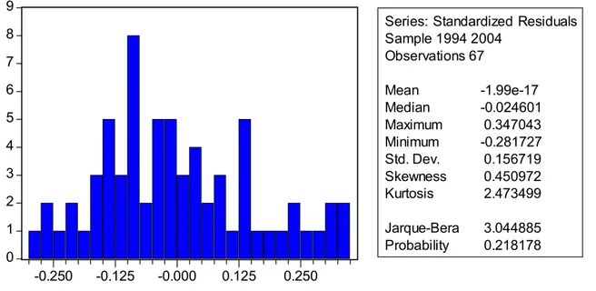
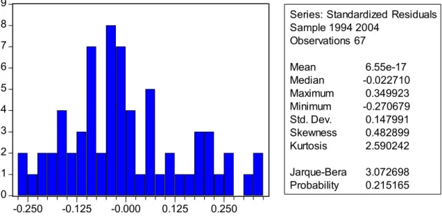
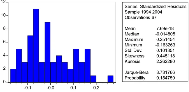
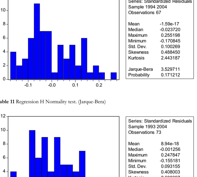
A Jarque-Bera normality test was done for all the regressions. The null hyphothesis of this test implies normality in the residuals. The results are in Appendix I (table 4, 5, 6 and 7) and Appen-dix II (table 8,9,10 and 11) for the level model and growth model respectively, and show no nor-mality problems, thus the null hypothesis can not be rejected, the residuals are normally distrib-uted. This test is crucial since a normality problem would give false test results (Gujarati 2003). When using GDP as the dependent variable we found out that we had a non-stationarity prob-lem in the models. This is a common probprob-lem in time series data. The probprob-lem occurs because GDP tends to rise over time. We may suspect a time pattern in the model yielding a spurious re-gression. To solve this problem we used GDP_Growth as the dependent variable in the second model. These results will also be presented and used to support the first model.
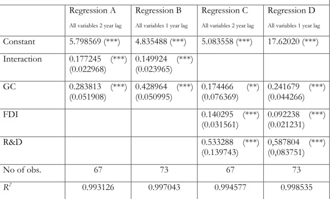
(***) significant at 1 % level. (**) significant at 5 % level. (*) significant at 10 % level. Std. error terms within parenthesis. Method: Pooled EGLS (Cross-section weights)
Regression A
In this model we test if the interaction term can enhance GDP, the explanatory variables are lagged 2 year. The estimated coefficient of the interaction term is significant and positively corre-lated to GDP, the coefficient is the elasticity of GDP with respect to the interaction term. Hence, if the interaction term increases with one percent, GDP increases with (on average) 0.177245 percent, all else equal. The coefficient for GFCF is significant and positively correlated to GDP, the coefficient is the elasticity of GDP with respect to GFCF. Hence, if the GFCF increases with one percent, GDP increases with (on average) 0.283813 percent, all else equal. This model has autocorrelation in the error terms, the Durbin-Watson stat is 1.043515 and should be 2 to ensure no first order autocorrelation.
Table 2 Econometric results data Regression A
All variables 2 year lag
Regression B
All variables 1 year lag
Regression C
All variables 2 year lag
Regression D
All variables 1 year lag
Constant 5.798569 (***) 4.835488 (***) 5.083558 (***) 17.62020 (***) Interaction 0.177245 (***) (0.022968) 0.149924 (***) (0.023965) GC 0.283813 (***) (0.051908) 0.428964 (***) (0.050995) 0.174466 (**) (0.076369) 0.241679 (***) (0.044266) FDI 0.140295 (***) (0.031561) 0.092238 (***) (0.021231) R&D 0.533288 (***) (0.139743) 0,587804 (***) (0,083751) No of obs. 67 73 67 73 R2 0.993126 0.997043 0.994577 0.998535
Regression B
In this model we test if the interaction term can enhance GDP, the explanatory variables are lagged 1 year. The estimated coefficient of the interaction term is significant and and positively correlated to GDP, the coefficient is the elasticity of GDP with respect to the interaction term. Hence, if the interaction term increases with one percent, GDP increases with (on average) 0.149924 percent, all else equal. The coefficient for GFCF is significant and positively correlated to GDP, the coefficient is the elasticity of GDP with respect to GFCF. Hence, if the GFCF in-creases with one percent, GDP inin-creases with (on average) 0.428964 percent, all else equal. This model has autocorrelation in the error terms, the Durbin-Watson stat is 1.120318 and should be 2 to ensure no first order autocorrelation.
Regression C
In this model we test for if R&D and FDI alone can enhance GDP, not accounting for the addi-tive effect they might have together when interacted, the explanatory variables are lagged 2 years. The estimated coefficient of R&D is significant and positively correlated to GDP, the coefficient is the elasticity of GDP with respect to R&D. Hence, if R&D increases with one percent, GDP increases with (on average) 0.533288 percent, all else equal. The coefficient for GFCF is signifi-cant and positively correlated to GDP, the coefficient is the elasticity of GDP with respect to GFCF. Hence, if the GFCF increases with one percent, GDP increases with (on average) 0.174466 percent, all else equal. The coefficient for FDI is significant and positively correlated to GDP, the coefficient is the elasticity of GDP with respect to FDI. Hence, if FDI increases with one percent, GDP increases with (on average) 0.140295 percent, all else equal. This model has autocorrelation in the error terms, the Durbin-Watson stat is 1.163818 and should be 2 to ensure no first order autocorrelation.
Regression D
In this model we test for if R&D and FDI alone can enhance GDP, not accounting for the addi-tive effect they might have together when interacted, the explanatory variables are lagged 1 year. The estimated coefficient of R&D is significant and positively correlated to GDP, the coefficient is the elasticity of GDP with respect to R&D. Hence, if R&D increases with one percent, GDP increases with (on average) 0,587804 percent, all else equal. The coefficient for GFCF is signifi-cant and positively correlated to GDP, the coefficient is the elasticity of GDP with respect to GFCF. Hence, if the GFCF increases with one percent, GDP increases with (on average) 0.241679 percent, all else equal. The coefficient for FDI is significant and positively correlated to GDP, the coefficient is the elasticity of GDP with respect to FDI. Hence, if FDI increases with one percent, GDP increases with (on average) 0.092238 percent, all else equal. This model has autocorrelation in the error terms, the Durbin-Watson stat is 1.365294 and should be 2 to ensure no first order autocorrelation.
For all these econometric equations (regression A,B,C and D) the R-square value is very high and close to one (99%). This suggests that the Sample Regression Function (SRF) fits the Population Regression Function (PRF) very well. This could be due to the fact that we have few tions, due to lagging, and many explanatory variables, which gives us low d.f. When the observa-tions are few and there are many explanatory variables, there is a tendency that the SRF fit well to PRF, showing an extremely high R-square. Therefore, removing an explanatory variable will in-crease the degrees of freedom. Therefore, we conduct another regression with the interaction term alone as the explanatory variable. The results are in Appendix III, table 13, and the model is still consistent with high R-square (99%). The interaction term is still significant and positively correlated to level GDP. We assume that the SRF fits very well to the PRF in our model since by increasing the degrees of freedom we still have a high R-square.
Empirical Framework
Second model test results
(***) significant at 1 % level. (**) significant at 5 % level. (*) significant at 10 % level. Std. error terms within parenthesis. Method: Pooled EGLS (Cross-section weights)
These models are a Lin-log model. The beta coefficient should be interpreted as follows:
β =∆Y/(∆X/X) (4.3)
where, as usual, ∆ denotes a small change. Equation (4.3) can be written, equivalently, as
∆Y = β(∆X/X) (4.3.1)
This equation states that the absolute change in Y ( = ∆Y) is equal to slope times the relative change in X. If the latter is multiplied by 100, then 4.3.1 gives the absolute change in Y for a per-centage change in X. Thus, if (∆X/X) changes by 0.01 unit (or 1 percent), the absolute change in Y is 0.01(β); if in an application one finds that β2 = 500, the absolute change in Y is (0.01)(500) = 5.0. β is the respectively corresponding variable coefficient in our models. (Gujarati 2003)
Regression E modified for GDP_growth
In this model we test if the interaction term can enhance GDP_Growth, the explanatory vari-ables are lagged 2 years. The estimated coefficient of the interaction term is significant and posi-tively correlated to GDP_Growth, a 1 unit increase in the interaction term increases GDP_Growth (0.300001/100) units, all else equal. The coefficient for GFCF is not significant. The This model has autocorrelation in the error terms, the Durbin-Watson stat is 1.358766 and should be 2 to ensure no first order autocorrelation.
Regression F modified for GDP_growth
In this model we test if the interaction term can enhance GDP_Growth, the explanatory vari-ables are lagged 1 year. The estimated coefficient of the interaction term is significant and posi-Table 3 Econometric results data
Regression E
All variables 2 year lag
Regression F
All variables 1 year lag
Regression G
All variables 2 year lag
Regression H
All variables 1 year lag
Constant -0.218569 -0.513284 -0.388492 -0.789801 Interaction 0.030001 (*) (0.015473) 0.026934 (*) (0.014763) GC -0.004498 (0.029130) 0.034009 (0.022405) -0.040039 (0.040447) -0.044585 (0.030299) FDI 0.018533 (0.018325) 0,009371 (0.014770) R&D 0.133230 (0.084553) 0.226112 (***) (0.059863) No of obs. 67 73 67 73 R2 0.128614 0.211468 0.146113 0.307782
tively correlated to GDP_Growth, a 1 unit increase in the interaction term increases GDP_Growth (0.026934/100) units, all else equal. The coefficient for GFCF is not significant. This model has autocorrelation in the error terms, the Durbin-Watson stat is 1.416965 and should be 2 to ensure no first order autocorrelation.
Regression G modified for GDP_growth
In this model we test for if R&D and FDI alone can enhance GDP, not accounting for the addi-tive effect they might have together when interacted, the explanatory variables are lagged 2 years. The estimated coefficient for R&D is significant not significant. The coefficient for Net FDI is not significant. The coefficient for GFCF is not significant. This model has autocorrelation in the error terms, the Durbin-Watson stat is 1.379687 and should be 2 to ensure no first order auto-correlation.
Regression H modified for GDP_growth
In this model we test for if R&D and FDI alone can enhance GDP, not accounting for the addi-tive effect they might have together when interacted, the explanatory variables are lagged 1 year. The estimated coefficient for R&D is significant, a 1 unit increase of R&D increases GDP_Growth (0.226112/100) units, all else equal. The coefficient for Net FDI is not significant. The coefficient for GFCF is not significant. This model has autocorrelation in the error terms, the Durbin-Watson stat is 1.580786 and should be 2 to ensure no first order autocorrelation. In regression E,F,G and H, the R-square is low, meaning that the fit of the SRF to the PRF is poor. This is because GDP_growth fluctuates more over time, compared to the level GDP.
For the regressions E,F,G and H. The R-square values are low and fluctuates from 12 % to 30 %. In regression E, 12 % of changes in GDP growth can be explanined by the changes in the inter-action term, since the estimated coefficient is significant. The estimated coefficient for the ex-planatory variable (GC) is not significant in this regression. In regression F, 21 % of changes in GDP growth can be explained by the changes in the interaction term, since the the estimated co-efficient is significant. The estimated coco-efficient for the explanatory variable (GC) is not signifi-cant in this regression. In regression H, 30% of the changes in GDP growth are explained by the changes in R&D spending, since the estimated coefficient is significant. The estimated coeffi-cients for the other explanatory variables are not significant in this regression.
Analysis
5
Analysis
In this section we are going to analyze the results that were presented in the previous section in an attempt to tie the results, supported by the descriptive statistics, to the theoretical framework.
When interacting net FDI and R&D, we assume that the effect of FDI in technology transfer and spillover in the host economy is high when the level of R&D in the host economy is also high. Meaning that when interacting the two variables and the estimated coefficient is positive and sig-nificant, there is a possibility of spillover effect of net FDI to the host economy through a multi-plier process. This implies that there is a complementary effect of Net FDI and R&D on growth. This result suggests that technological progress (A) is enhanced, since the rate of technology dif-fusion is greater in the host economy when the level of domestic knowledge driven by R&D is high. This is significant and positively correlated in model A,B, E and F.
In the regression models A-B the interaction term (R&D*FDI) is positively correlated to GDP as expected. This implies that when R&D and net FDI for the previous years were both high the GDP level is magnified in the current year. We see the same pattern in the growth model (regres-sion E andF), that unveils to us that the rate of economic growth has been positively affected by the interaction term. This means the higher the interaction term the higher the rate of techno-logical progress(A) and the higher the growth rate of GDP (equation 2.1), all else equal. Giving that the level GDP has been changing during this period, one can assume that this is due to eco-nomic growth. When the level of GDP from a previous year is lower than the current year we as-sume positive economic growth, when the level GDP is greater in the previous year than in the current year we assume negative economic growth. This explains why the level GDP has been changing, as seen in figure 3. From table 1 it is possible to see that countries with high net FDI and R&D were able to record a high level of GDP per capita at the end of the period (2004). This is the case for Czech Republic and Hungary. Slovenia that had the highest R&D per capita through the period 1992-2004, but low inflows of FDI per capita during this period, was able to record the highest level of GDP per capita in 2004. This was due to very high absorptive capacity and the fact that this country is more innovative. This implies that even though net FDI was not as high as Czech Republic and Hungary, they were still able to absorb it to a greater extent when compared to the other countries. Therefore our results indicate that Slovenia has a very high ab-sorptive capacity and can be explained further because they are more innovative.
GC (domestic investment) was also found to be significant and positively correlated to GDP in regression A,B, C and D. This is in line with economic theory since investment is a component of GDP and we expected it to be positively correlated to GDP, according to the national income accounting equation. In the growth model GC is negatively correlated to GDP growth. This re-sult is insignificant and therefore we will not draw any further analysis on this rere-sult.
In regression C,D and H we find that R&D is able to affect GDP (C,D) and GDP_growth (H) positively, as expected. This means that the higher the level of R&D the higher the rate of tech-nological progress (A) on which growth depends according to the growth accounting equation (2.1). We found theory to be consistent with the growth model (regression G and H). For the level GDP model (regression C and D), R&D spending can be assumed to be investments either by firms or by governments. This would increase the level of output through efficiency, therefore the level GDP would increase.
Net FDI is found to positively affect the level of GDP in regression C and D. This results are statistically significant. Net FDI is a component of GFCF, therefore an increase in Net FDI will increase GFCF leading to a increase in the level of GDP. When Net FDI complements domestic investment, for example supplies inputs to domestic firms, crowding in occurs. Since the result is significant we assume that net FDI was complementing domestic investment. For the growth
model (regression G and H) the coefficient estimate of net FDI was insignificant. Therefore we will not further analyse these results.
The high R-square of 99%, suggests that 99% of the changes in level GDP are explained by the interaction term as explained in Regression A and B. The Adjusted R-square is also extremely high in both models. Our regression result of an extremely high R-square can be explained be-cause we use level GDP as the dependent variable which is a variable that doesn’t fluctuate very much over time. The explanatory variable does not fluctuate very much over time either, we use net FDI stock and R&D stock. This is one of the reasons why the overall goodness of fit (R-square) we have in the level GDP model is very high.
In the growth model the estimated coefficient for the interaction term is significant and positively correlated to GDP growth (regression E,F). The R-square in these regression E,F is 12% and 21% respectively. This means that 12 % of the GDP growth in these economies is explained by the changes in the interaction term and that 21% of the GDP growth in these economies is ex-plained by the interaction term, for regression E and F respectively. The results add support to the main findings of this thesis, since a high R-square of the level GDP model adds uncertainty of the significance in of the explanatory variables in this model. In the GDP growth model the interaction term is still significant and the R-square is low, meaning that the significance is more certain and strengthens the findings of the level GDP model.
Conclusion
6
Conclusion
The purpose of this thesis was to analyze whether the technological spillover effect of FDI on economic growth in the CEE Countries and the Baltic States is conditioned on the level of do-mestic R&D or not. Given that FDI and R&D are both sources of technological progress, it is interesting to investigate if FDI alone can spur growth to these economies or whether the extent to which FDI induces spillovers depends on the absorptive capacity, proxied by the level of R&D in these economies.
The results show a significant and positive correlation between R&D and FDI when interacted, were R&D is proxied as the level of the host economy’s “knowledge” and FDI, through a spill-over effect, a source of external technology. This implies that FDI and R&D are good sources of technological progress, since according to the results, it would increase A in the economy, creat-ing long-term economic growth. The results are inline with what we expected. R&D is a good proxy for domestic “knowledge” R&D activities can be stimulated when companies are em-braced with an institutional framework that will protect their new innovations. If this is not the case, few companies or no companies would engage in R&D activities. According to Romer (1990a) this is easy to understand since the companies regard R&D spending as investments that will bear fruit in the future. With no convincing institutional framework companies would not engaged in R&D spending, and little or no technological progress would occur. From the point of view of the transition economies of the CEE countries and the Baltic States, one can argue that going from a command economy to a market economy was very much a struggle against time in achieving those institutions that would creditably protect R&D spending. What can surely be said is that these countries posses the required threshold of human capital to engage in R&D activities. The former socialist systems were known to have a highly educated labour force. Bor-entszein et al. (1998) presented a similar conclusion by conditioning the spillover effect of FDI on human capital which they use as a proxy for absorptive capacity.
The results of this thesis would not certainly be the same if a different sample of countries were chosen since the human capital threshold has to be fullfiled and the R&D level has to be high in the economy, as well as FDI. Putting these prerequisites would ensure that the spillover effect of FDI would be maximized and this would accelerate growth of the host country leading to an up-grade of the economy.
6.1
Further Studies
In the study by Borentszein et al. (1998) the threshold level of human capital or the minimum level of human capital for a host economy is calculated from where a country starts to benefit from FDI spillovers. It would be interesting to investigate, if there is a threshold level of R&D, or to put it differently a minimum level of R&D were host economies that receive inflows of FDI will maximize the increase in technological progress (A) due to the technological spillovers of FDI. Thus an advice can be given to developing countries to gain access to higher human capital and R&D spending, that would enable them to reap the full benefits of FDI and accelerate their catch up process.
Another interesting issue could be to make a panel data study with country specific betas for the interaction term. When comparing the betas, it should be possible to spot the differences in elas-ticities or the slope among countries with respect to R&D spending and FDI inflows.
7
References
Alfaro L, Areendam C, Kalemli-Ozcan S, Sayek S (2004), FDI and economic growth: the role of local financial markets, Journal of international economics 64, 89-112
Blomström, M., and Kokko A.(2003) The economics of foreigne direct investment incentives, Working Paper No. 9489, Cambridge, Mass. National Bureau of Economic Analysis. Borensztein, E., De Gregorio, J., and J.W. Lee, (1998), “How does foreign investment affect
growth?” Journal of International Economics, 45.
Cohen WM, Levinthal DA.(1989) Innovation and Learning: The Two Faces of R & D. Wesley M. Cohen. Daniel A. Levinthal. The Economic Journal, Vol. 99, No. 397, 569-596. Sep., 1989
Easterly, W.and Levine, R. (2001), What have we learned from a decade of empirical research on growth? It’s not factor accumulation: stylised facts and growth models, the World Bank Economic Review, 15(2), 177-219.
European Bank for Reconstruction and Development. (2004). Transition report 2004 – Infrastructure. European Bank for Reconstruction and Development Publications. Eurostat (2006), Gross domestic expenditure on R&D (GERD), retrieved 2006-10-07 from
http://epp.eurostat.ec.europa.eu/portal/page?_pageid=1996,39140985&_dad=porta l&_schema=PORTAL&screen=detailref&language=en&product=STRIND_INNO RE&root=STRIND_INNORE/innore/ir021
Fabry, Nathalie (2000) The Role of Inward-FDI in the Transition Countries of Europe : An Ana-lytical Framework, Working Paper n° WP 2000-4, Université de Marne-la-Vallée, Département Aires Culturelles et Politiques, Laboratoire GREET – ICARIE, bâti-ment Albert Camus, 2 rue de la butte verte, F-93166 Noisy-le-Grand (France)
Grossman, G. and E. Helpman. (1991). Innovation and Growth in the Global Economy. Cam-bridge, MA: MIT Press. L. Alfaro et al. / Journal of International Economics 64 (2004) 89–112
Gujarati, D.N. (2003). Basic Econometrics. McGraw-Hill Higher Education. Fourth Edition Javorcik, B (2004) Does foreign direct investments increase the productivity of domestic firms?
In search of spillover through backward linkages, American Economic Review, 94(3) Johnson, A. (2005) Host Country Effects of Foreign Direct Investment. Dissertation Series of
JIBS Jönköping International Business School
Krugman, P. (1991) ”Geography and Trade”, Leuven; Leuven University Press.
Lucas, R.E. (1988), On the mechanics of economic development, Journal of Monetary Econom-ics, 22(1), 3-34
Mansfield, E. and M. Romeo. (1980). "Technology Transfer to Overseas Subsidiaries by U.S. Based Firms". Quarterly Journal of Economics, 95: 737-750